1.0 INTRODUCTION
For realizing the maximum effectiveness of the missile and performing a precision strike on the target, not only does the missile need to hit the target accurately, but it is also expected to attack the target from a specified angle(Reference Xinsan, Lixin and Xiaohu1,Reference Erer and Tekin2) . Therefore, it is of great practical engineering significance to study the guidance law with impact-angle constraints(Reference Taub and Shima3).
There are many methods for designing the guidance law with impact-angle constraint at present. Based on the idea of proportional guidance, Ref. (Reference Lee, Kim and Tahk4) designs a new type of bias proportional guidance law with impact-angle constraints, its bias term is a function of the residual time and impact-angle error. Based on the optimal control theory, and constrained by zero miss-distance and zero impact-angle error, Ref. (Reference Wang, Lin and CHENG5) obtains the close-form solution of optimal guidance law with impact-angle constraints by using Schwartz inequality. Based on the theory of Model Predictive Static Programming (MPSP), the control quantity of the angle is updated iteratively to satisfy the constraint conditions of impact-angle in Ref. (Reference Wang, Wang and LIN6). Based on the theory of sliding mode control, Ref. (Reference Zhang, Liu and LI7) designs the guidance law with impact-angle constraints and designs the extended state observer to estimate target maneuvering information.
Guidance law based on the theory of sliding mode control is very robust to external interference(Reference Wang and Hong8), so it is widely used in the design of guidance law. Ref. (Reference Xiong, Wang and Wang9) designs the sliding surface based on the non-singular fast terminal sliding mode function and applies fast exponential reaching law to design the guidance law in 2D space law with impact-angle constraints. Ref. (Reference Zhao, Zhou and Lu10) proposes an integral sliding surface with finite time convergence and also applies fast exponential reaching law to design the guidance law for attacking maneuvering target in 2D space with impact-angle constraint and makes adaptive estimation for the upper bound of unknown maneuvering target. But Ref. (Reference Xiong, Wang and Wang9) and (Reference Zhao, Zhou and Lu10) only design the guidance law in 2D space and the coupling relation between channels in 3D space is not considered, which makes the design of the guidance law less practical. Ref. (Reference Zhao, Li and Liu11) proposes a 3D finite-time sliding mode guidance law with impact-angle constraints. The model of guidance system is not decoupled during the design process, and this guidance law can only be used to attack stationary targets. Ref. (Reference Si and Song12) applies the fast-double exponential reaching law to design 3D forward sliding mode guidance law and ensures that the system can converge quickly to the sliding surface, but this guidance law does not take the problem of impact-angle constraints into consideration. In addition, all the above References study the first-order sliding mode guidance law while the second-order sliding mode guidance has the advantages of strong chattering suppression and strong robustness(Reference Arie13). So, the 3D finite-time guidance law with impact-angle constraints based on the theory of second-order sliding mode variable structure control is of great practical engineering value.
In this paper, a complete three-dimensional guidance system model is established and there is no need to decouple the model. Then, the second-order sliding mode guidance law is designed by selecting the non-singular terminal sliding mode surface, and also, the nonhomogeneous disturbance observer is designed, which estimate and compensate coupling terms of unknown target maneuvering information and line-of-sight angle to avoid the singular problem in traditional terminal sliding mode guidance law. Finally, the stability and finite-time convergence of the proposed guidance law are proved mathematically.
The advantages of the guidance law proposed in this paper are as following: ① 3D coupling terms are considered in the design of guidance law, and there is no need to decouple the system model. ② The nonhomogeneous disturbance observer is designed to estimate the total disturbance caused by the coupling of target maneuvering information and line-of-sight angle and prior information of target is not needed. ③ The second-order sliding mode guidance law is designed by selecting the non-singular terminal sliding mode surface, which converges fast and can restrain chattering phenomenon effectively. ④ The guidance law proposed in the paper can be used to attack maneuvering targets in 3D space with impact-angle constraints and has much value for engineering application.
2.0 3D SPACE TERMINAL GUIDANCE SYSTEM MODEL
Considering the case of a missile attacking a ground maneuvering target in 3D space, the relative motion relationship between the missile and the target is shown in Fig. 1.
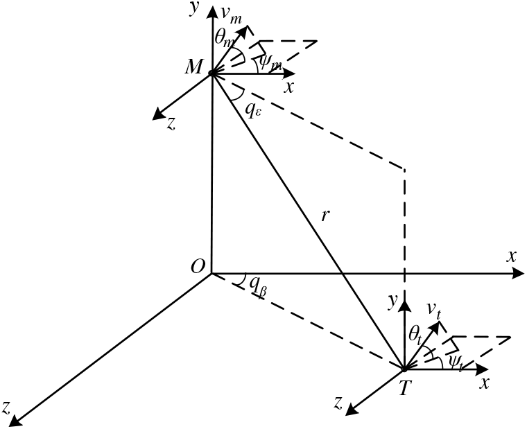
Figure 1. Relative motion between missile and target.
In Fig. 1, Oxyz is the ground inertial coordinate system; M and T stand for the missile and the target respectively; r stands for the line of sight between missile and target;
 $q_{\varepsilon }$
and
$q_{\varepsilon }$
and
 $q_{\beta }$
stand for line-of-sight dip angle and line-of-sight drift angle, respectively; and the direction is defined as follows:
$q_{\beta }$
stand for line-of-sight dip angle and line-of-sight drift angle, respectively; and the direction is defined as follows:
 $q_{\varepsilon }$
is positive when r is above the horizontal plane Oxz;
$q_{\varepsilon }$
is positive when r is above the horizontal plane Oxz;
 $q_{\beta }$
is positive when the ox axis rotates anticlockwise on the projection of r on the plane Oxz.
$q_{\beta }$
is positive when the ox axis rotates anticlockwise on the projection of r on the plane Oxz.
 ${v}_{m}$
is the velocity of missile,
${v}_{m}$
is the velocity of missile,
 $\theta _{m}$
and
$\theta _{m}$
and
 $\varphi _{m}$
stand for ballistic inclination angle and ballistic deflection angle. The direction is defined as follows:
$\varphi _{m}$
stand for ballistic inclination angle and ballistic deflection angle. The direction is defined as follows:
 $\theta _{m}$
is positive when
$\theta _{m}$
is positive when
 ${v}_{m}$
is above the horizontal plane;
${v}_{m}$
is above the horizontal plane;
 $\varphi _{m}$
is positive when the ox axis rotates anticlockwise on the projection of
$\varphi _{m}$
is positive when the ox axis rotates anticlockwise on the projection of
 ${v}_{m}$
on the plane Oxz.
${v}_{m}$
on the plane Oxz.
 ${v}_{t}$
is the velocity of target.
${v}_{t}$
is the velocity of target.
 $\theta _{t}$
and
$\theta _{t}$
and
 $\varphi _{t}$
respectively stands for course angle in pitching direction and in horizontal direction. Definition of their direction is the same as that of ballistic inclination angle and ballistic deflection angle. According to Fig. 1, the relative motion equation of missile target in 3D space is:
$\varphi _{t}$
respectively stands for course angle in pitching direction and in horizontal direction. Definition of their direction is the same as that of ballistic inclination angle and ballistic deflection angle. According to Fig. 1, the relative motion equation of missile target in 3D space is:
 \begin{equation}
\left\{\begin{split}
\dot{r}& =v_{t} \left(\cos \theta _{t} \cos q_{\varepsilon } \cos \left(q_{\beta } -\varphi _{t} \right)+\sin \theta _{t} \sin q_{\varepsilon } \right)\\
&\quad-v_{m} \left(\cos \theta _{m} \cos q_{\varepsilon } \cos \left(q_{\beta } -\varphi _{m} \right)+\sin \theta _{m} \sin q_{\varepsilon } \right) \\
r\dot{q}_{\varepsilon } &=-v_{t} \left(\cos \theta _{t} \sin q_{\varepsilon } \cos \left(q_{\beta } -\varphi _{t} \right)-\sin \theta _{t} \cos q_{\varepsilon } \right) \\
&\quad+v_{m} \left(\cos \theta _{m} \sin q_{\varepsilon } \cos \left(q_{\beta } -\varphi _{m} \right)-\sin \theta _{m} \cos q_{\varepsilon } \right) \\ r\dot{q}_{\beta} \cos q_{\varepsilon } &=-v_{t} \cos \theta _{t} \sin \left(q_{\beta } -\varphi _{t} \right)+v_{m} \cos \theta _{m} \sin \left(q_{\beta } -\varphi _{m} \right)
\end{split}\right.
\end{equation}
\begin{equation}
\left\{\begin{split}
\dot{r}& =v_{t} \left(\cos \theta _{t} \cos q_{\varepsilon } \cos \left(q_{\beta } -\varphi _{t} \right)+\sin \theta _{t} \sin q_{\varepsilon } \right)\\
&\quad-v_{m} \left(\cos \theta _{m} \cos q_{\varepsilon } \cos \left(q_{\beta } -\varphi _{m} \right)+\sin \theta _{m} \sin q_{\varepsilon } \right) \\
r\dot{q}_{\varepsilon } &=-v_{t} \left(\cos \theta _{t} \sin q_{\varepsilon } \cos \left(q_{\beta } -\varphi _{t} \right)-\sin \theta _{t} \cos q_{\varepsilon } \right) \\
&\quad+v_{m} \left(\cos \theta _{m} \sin q_{\varepsilon } \cos \left(q_{\beta } -\varphi _{m} \right)-\sin \theta _{m} \cos q_{\varepsilon } \right) \\ r\dot{q}_{\beta} \cos q_{\varepsilon } &=-v_{t} \cos \theta _{t} \sin \left(q_{\beta } -\varphi _{t} \right)+v_{m} \cos \theta _{m} \sin \left(q_{\beta } -\varphi _{m} \right)
\end{split}\right.
\end{equation}
The dynamic equation of the missile is:
 \begin{equation}
\left\{\begin{split}
\dot{v}_{m} &=a_{x} \\
\dot{\theta}_{m} &=\frac{a_{y} }{v_{m} } \\
\dot{\varphi}_{m} &=-\frac{a_{z} }{v_{m} \cos \theta _{m} } \end{split}\right.
\end{equation}
\begin{equation}
\left\{\begin{split}
\dot{v}_{m} &=a_{x} \\
\dot{\theta}_{m} &=\frac{a_{y} }{v_{m} } \\
\dot{\varphi}_{m} &=-\frac{a_{z} }{v_{m} \cos \theta _{m} } \end{split}\right.
\end{equation}
Where,
 $a_{x} ,a_{y}$
and
$a_{x} ,a_{y}$
and
 $a_{z}$
are the three components of missile acceleration in velocity direction, normal velocity direction and lateral velocity direction. Most missiles have no thrust during the process of terminal guidance so the acceleration is caused by a combined external force acting on the missile.
$a_{z}$
are the three components of missile acceleration in velocity direction, normal velocity direction and lateral velocity direction. Most missiles have no thrust during the process of terminal guidance so the acceleration is caused by a combined external force acting on the missile.
Decompose the missile velocity
 ${v}_{m}$
on three axes of the ground inertial coordinate system Oxyz, the equation of missile motion in 3D space is written as:
${v}_{m}$
on three axes of the ground inertial coordinate system Oxyz, the equation of missile motion in 3D space is written as:
 \begin{equation}
\left\{\begin{split}
\dot{x}_{m} &=v_{m} \cos \theta _{m} \cos \varphi _{m} \\
\dot{y}_{m} &=v_{m} \sin \theta _{m} \\
\dot{z}_{m} &=-v_{m} \cos \theta _{m} \sin \varphi _{m} \end{split}\right.
\end{equation}
\begin{equation}
\left\{\begin{split}
\dot{x}_{m} &=v_{m} \cos \theta _{m} \cos \varphi _{m} \\
\dot{y}_{m} &=v_{m} \sin \theta _{m} \\
\dot{z}_{m} &=-v_{m} \cos \theta _{m} \sin \varphi _{m} \end{split}\right.
\end{equation}
Similarly, decompose the target velocity
 ${v}_{t}$
on the three axes of the ground inertial coordinate system Oxyz. The equation of target motion can be got.
${v}_{t}$
on the three axes of the ground inertial coordinate system Oxyz. The equation of target motion can be got.
Suppose that the rotational angular velocity of the line-of-sight coordinate system with respect to the inertial coordinate system on the ground is
 $\boldsymbol{\omega}$
. The components of the relative velocity of missile and target, the relative acceleration of missile and target, missile velocity and missile acceleration in the line-of-sight coordinate system are
$\boldsymbol{\omega}$
. The components of the relative velocity of missile and target, the relative acceleration of missile and target, missile velocity and missile acceleration in the line-of-sight coordinate system are
 $v_{r}$
,
$v_{r}$
,
 $\boldsymbol{\alpha}_{\bf{\it{r}}}$
,
$\boldsymbol{\alpha}_{\bf{\it{r}}}$
,
 $\bf{\it{v}}_{\bf{\it{m}}}$
and
$\bf{\it{v}}_{\bf{\it{m}}}$
and
 $\bf{\it{a}}_{\bf{\it{m}}}$
. According to the Coriolis effect, the following equation is written as:
$\bf{\it{a}}_{\bf{\it{m}}}$
. According to the Coriolis effect, the following equation is written as:
 \begin{equation}
\left\{\begin{split}
\bf{\it{a}}_{\bf{\it{r}}} &=\frac{\partial \bf{\it{v}}_{\bf{\it{r}}} }{\partial \bf{\it{t}}} +\boldsymbol{\omega} \times \bf{\it{v}}_{\bf{\it{r}}} \\
\bf{\it{a}}_{\bf{\it{m}}} &=\frac{\partial \bf{\it{v}}_{\bf{\it{m}}} }{\partial \bf{\it{t}}} +\boldsymbol{\omega} \times \bf{\it{v}}_{\bf{\it{m}}} \end{split}\right.
\end{equation}
\begin{equation}
\left\{\begin{split}
\bf{\it{a}}_{\bf{\it{r}}} &=\frac{\partial \bf{\it{v}}_{\bf{\it{r}}} }{\partial \bf{\it{t}}} +\boldsymbol{\omega} \times \bf{\it{v}}_{\bf{\it{r}}} \\
\bf{\it{a}}_{\bf{\it{m}}} &=\frac{\partial \bf{\it{v}}_{\bf{\it{m}}} }{\partial \bf{\it{t}}} +\boldsymbol{\omega} \times \bf{\it{v}}_{\bf{\it{m}}} \end{split}\right.
\end{equation}
In this equation,
 \begin{align*}
\boldsymbol{\omega} &=\left[\begin{array}{c@{\,\,}c@{\,\,}c} {0} & {-\dot{q}_{\varepsilon } } & {\dot{q}_{\beta} \cos q_{\varepsilon } } \\[4pt] {\dot{q}_{\varepsilon } } & {0} & {-\dot{q}_{\beta} \sin q_{\varepsilon } } \\[4pt] {-\dot{q}_{\beta} \cos q_{\varepsilon } } & {\dot{q}_{\beta} \sin q_{\varepsilon } } & {0} \end{array}\right],\quad \bf{\it{v}}_{\bf{\it{r}}} =\left[\begin{array}{c} {\dot{r} } \\[4pt] {r\dot{q}_{\varepsilon } } \\[4pt] {-r\dot{q}_{\beta} \cos q_{\varepsilon } } \end{array}\right],\\[6pt]
\bf{\it{v}}_{\bf{\it{m}}} &=\left[\begin{array}{c} {v_{m} \left(\cos \theta _{m} \cos q_{\varepsilon } \cos \left(q_{\beta } -\varphi _{m} \right)+\sin \theta _{m} \sin q_{\varepsilon } \right)} \\[4pt] {-v_{m} \left(\cos \theta _{m} \sin q_{\varepsilon } \cos \left(q_{\beta } -\varphi _{m} \right)-\sin \theta _{m} \cos q_{\varepsilon } \right)} \\[4pt] {v_{m} \cos \theta _{m} \sin \left(q_{\beta } -\varphi _{m} \right)} \end{array}\right]
\end{align*}
\begin{align*}
\boldsymbol{\omega} &=\left[\begin{array}{c@{\,\,}c@{\,\,}c} {0} & {-\dot{q}_{\varepsilon } } & {\dot{q}_{\beta} \cos q_{\varepsilon } } \\[4pt] {\dot{q}_{\varepsilon } } & {0} & {-\dot{q}_{\beta} \sin q_{\varepsilon } } \\[4pt] {-\dot{q}_{\beta} \cos q_{\varepsilon } } & {\dot{q}_{\beta} \sin q_{\varepsilon } } & {0} \end{array}\right],\quad \bf{\it{v}}_{\bf{\it{r}}} =\left[\begin{array}{c} {\dot{r} } \\[4pt] {r\dot{q}_{\varepsilon } } \\[4pt] {-r\dot{q}_{\beta} \cos q_{\varepsilon } } \end{array}\right],\\[6pt]
\bf{\it{v}}_{\bf{\it{m}}} &=\left[\begin{array}{c} {v_{m} \left(\cos \theta _{m} \cos q_{\varepsilon } \cos \left(q_{\beta } -\varphi _{m} \right)+\sin \theta _{m} \sin q_{\varepsilon } \right)} \\[4pt] {-v_{m} \left(\cos \theta _{m} \sin q_{\varepsilon } \cos \left(q_{\beta } -\varphi _{m} \right)-\sin \theta _{m} \cos q_{\varepsilon } \right)} \\[4pt] {v_{m} \cos \theta _{m} \sin \left(q_{\beta } -\varphi _{m} \right)} \end{array}\right]
\end{align*}
Expanding the first equation of Equation (4) produces:
 \begin{equation}
\left\{\begin{split}
a_{tr} -a_{mr} &=\ddot{r} -r\dot{q}_{\varepsilon}^{2} -r\dot{q}_{\beta }^{2} \cos q_{\varepsilon } ^{2} \\
a_{t\theta } -a_{m\theta } &=2\dot{r} \dot{q}_{\varepsilon } +r\dot{q}_{\varepsilon } +r\dot{q}_{\beta }^{2} \sin q_{\varepsilon } \cos q_{\varepsilon }\\
a_{t\varphi } -a_{m\varphi } &=-2\dot{r} \dot{q}_{\beta} \cos q_{\varepsilon } -r\dot{q}_{\beta} \cos q_{\varepsilon } +2r\dot{q}_{\varepsilon } \dot{q}_{\beta} \sin q_{\varepsilon } \end{split}\right.
\end{equation}
\begin{equation}
\left\{\begin{split}
a_{tr} -a_{mr} &=\ddot{r} -r\dot{q}_{\varepsilon}^{2} -r\dot{q}_{\beta }^{2} \cos q_{\varepsilon } ^{2} \\
a_{t\theta } -a_{m\theta } &=2\dot{r} \dot{q}_{\varepsilon } +r\dot{q}_{\varepsilon } +r\dot{q}_{\beta }^{2} \sin q_{\varepsilon } \cos q_{\varepsilon }\\
a_{t\varphi } -a_{m\varphi } &=-2\dot{r} \dot{q}_{\beta} \cos q_{\varepsilon } -r\dot{q}_{\beta} \cos q_{\varepsilon } +2r\dot{q}_{\varepsilon } \dot{q}_{\beta} \sin q_{\varepsilon } \end{split}\right.
\end{equation}
Where,
 $a_{tr} ,a_{t\theta } ,a_{t\varphi }$
and
$a_{tr} ,a_{t\theta } ,a_{t\varphi }$
and
 $a_{mr} ,a_{m\theta } ,a_{m\varphi }$
respectively stand for the components of the target and missile acceleration on the three axes of the line-of-sight coordinate system.
$a_{mr} ,a_{m\theta } ,a_{m\varphi }$
respectively stand for the components of the target and missile acceleration on the three axes of the line-of-sight coordinate system.
Expand the second equation of Equation (4). Substitute Equation (2) in and simplify, the transformation relation between
 $a_{y}$
,
$a_{y}$
,
 $a_{z}$
and
$a_{z}$
and
 $a_{m\theta }$
,
$a_{m\theta }$
,
 $a_{m\varphi }$
can be got:
$a_{m\varphi }$
can be got:
 \begin{equation}
\left\{\begin{split}
a_{y} &=\dfrac{\cos \left(q_{\beta } -\varphi _{m} \right)a_{m\theta } -\sin \left(q_{\beta } -\varphi _{m} \right)\sin q_{\varepsilon } a_{m\varphi } }{\sin \theta _{m} \sin q_{\varepsilon } +\cos \theta _{m} \cos q_{\varepsilon } \cos \left(q_{\beta } -\varphi _{m} \right)} \\
a_{z} &=\dfrac{a_{m\varphi } +\sin \theta _{m} \cos \left(q_{\beta } -\varphi _{m} \right)a_{m\theta } }{\cos \left(q_{\beta } -\varphi _{m} \right)} \end{split}\right.
\end{equation}
\begin{equation}
\left\{\begin{split}
a_{y} &=\dfrac{\cos \left(q_{\beta } -\varphi _{m} \right)a_{m\theta } -\sin \left(q_{\beta } -\varphi _{m} \right)\sin q_{\varepsilon } a_{m\varphi } }{\sin \theta _{m} \sin q_{\varepsilon } +\cos \theta _{m} \cos q_{\varepsilon } \cos \left(q_{\beta } -\varphi _{m} \right)} \\
a_{z} &=\dfrac{a_{m\varphi } +\sin \theta _{m} \cos \left(q_{\beta } -\varphi _{m} \right)a_{m\theta } }{\cos \left(q_{\beta } -\varphi _{m} \right)} \end{split}\right.
\end{equation}
During the terminal guidance stage, the component of the relative acceleration of missile and target in the line-of-sight coordinate system is quite small, so setting the component
 $a_{mr}$
of missile acceleration in the line-of-sight direction as 0. In order to make the rate of change of ballistic inclination angle
$a_{mr}$
of missile acceleration in the line-of-sight direction as 0. In order to make the rate of change of ballistic inclination angle
 $\dot{q}_{\varepsilon }$
and ballistic deflection angle
$\dot{q}_{\varepsilon }$
and ballistic deflection angle
 $\dot{q}_{\beta}$
converge to 0 in finite time, and to make ballistic inclination angle
$\dot{q}_{\beta}$
converge to 0 in finite time, and to make ballistic inclination angle
 $q_{\varepsilon }$
and ballistic deflection angle
$q_{\varepsilon }$
and ballistic deflection angle
 $q_{\beta }$
converge to expected value
$q_{\beta }$
converge to expected value
 $q_{\varepsilon d}$
and
$q_{\varepsilon d}$
and
 $q_{\beta d}$
in finite time, the missile acceleration in line-of-sight normal direction
$q_{\beta d}$
in finite time, the missile acceleration in line-of-sight normal direction
 $a_{m\theta }$
and in lateral direction
$a_{m\theta }$
and in lateral direction
 $a_{m\varphi }$
are designed in this paper by using the second and third equations of Equation (5).
$a_{m\varphi }$
are designed in this paper by using the second and third equations of Equation (5).
3.0 THE DESIGN OF GUIDANCE LAW
Aiming at the problem that the missile attacks the ground maneuvering target at the specified angle in 3D space, this part designs a nonsingular fast terminal second-order sliding mode guidance law with impact-angle constraints. Firstly, the state equation of the 3D system with impact-angle constraints is given. Then, the second-order sliding mode guidance law is designed by selecting the non-singular terminal sliding mode surface, which ensures that the chattering phenomenon is effectively suppressed while the system converges rapidly. At last, the nonhomogeneous disturbance observer is designed for the target maneuvering information and the coupling term of line-of-sight angle in the system to estimate and compensate the total disturbance in the system.
3.1 Design goals
When the missile hits the target, the missile angle of attack can be approximately 0. According to Ref. (Reference Sun, Wang and YI14), the problem of missile impact-angle constraints can be transformed into the problem of line-of-sight tracking.
Suppose that the excepted line-of-sight dip angle and line-of-sight drift angle at the time the missile hits the target are respectively
 $q_{\varepsilon d}$
and
$q_{\varepsilon d}$
and
 $q_{\beta d}$
, make
$q_{\beta d}$
, make
 $x_{1} =q_{\varepsilon } -q_{\varepsilon d}$
,
$x_{1} =q_{\varepsilon } -q_{\varepsilon d}$
,
 $x_{2} =\dot{q}_{\varepsilon }$
,
$x_{2} =\dot{q}_{\varepsilon }$
,
 $x_{3} =q_{\beta } -q_{\beta d}$
,
$x_{3} =q_{\beta } -q_{\beta d}$
,
 $x_{4} =\dot{q}_{\beta}$
. Simplify the second and third equations in Equation (5), the system state equation in 3D space can be shown as:
$x_{4} =\dot{q}_{\beta}$
. Simplify the second and third equations in Equation (5), the system state equation in 3D space can be shown as:
 \begin{equation}
\left\{\begin{split}
\dot{x}_{1} &=x_{2} \\
\dot{x}_{2} &=\frac{-2\dot{r} x_{2} }{r} +d_{\theta } -\frac{a_{m\theta } }{r} \\
\dot{x}_{3} &=x_{4} \\
\dot{x}_{4} &=\frac{-2\dot{r} x_{4} }{r} +d_{\varphi } +\frac{a_{m\varphi } }{r\cos q_{\varepsilon } } \end{split}\right.
\end{equation}
\begin{equation}
\left\{\begin{split}
\dot{x}_{1} &=x_{2} \\
\dot{x}_{2} &=\frac{-2\dot{r} x_{2} }{r} +d_{\theta } -\frac{a_{m\theta } }{r} \\
\dot{x}_{3} &=x_{4} \\
\dot{x}_{4} &=\frac{-2\dot{r} x_{4} }{r} +d_{\varphi } +\frac{a_{m\varphi } }{r\cos q_{\varepsilon } } \end{split}\right.
\end{equation}
In this equation,
 $d_{\theta }$
and
$d_{\theta }$
and
 $d_{\varphi }$
are the total disturbance caused by the coupling term of maneuvering information of the target and the line-of-sight angle in the normal direction and lateral direction of line-of- sight respectively. The expressions are respectively:
$d_{\varphi }$
are the total disturbance caused by the coupling term of maneuvering information of the target and the line-of-sight angle in the normal direction and lateral direction of line-of- sight respectively. The expressions are respectively:
 \begin{equation}
\left\{\begin{split} {d_{\theta } =-x_{4} ^{2} \sin q_{\varepsilon } \cos q_{\varepsilon } +\frac{a_{t\theta } }{r} } \\ {d_{\varphi } =2x_{2} x_{4} \tan q_{\varepsilon } -\frac{a_{t\varphi } }{r\cos q_{\varepsilon } } } \end{split}\right.
\end{equation}
\begin{equation}
\left\{\begin{split} {d_{\theta } =-x_{4} ^{2} \sin q_{\varepsilon } \cos q_{\varepsilon } +\frac{a_{t\theta } }{r} } \\ {d_{\varphi } =2x_{2} x_{4} \tan q_{\varepsilon } -\frac{a_{t\varphi } }{r\cos q_{\varepsilon } } } \end{split}\right.
\end{equation}
The purpose of this part to design the guidance law is to make system Equation (7) converge to 0 in a finite time by designing the missile acceleration in line-of-sight normal direction
 $a_{m\theta }$
and the missile acceleration in line-of-sight lateral direction
$a_{m\theta }$
and the missile acceleration in line-of-sight lateral direction
 $a_{m\varphi }$
, and to estimate and compensate the total disturbance
$a_{m\varphi }$
, and to estimate and compensate the total disturbance
 $a_{m\theta }$
and
$a_{m\theta }$
and
 $a_{m\varphi }$
in the system by designing an nonhomogeneous disturbance observer.
$a_{m\varphi }$
in the system by designing an nonhomogeneous disturbance observer.
3.2 Second-order sliding mode guidance law based on fast terminal sliding surface
According to Equation (7), choosing the fast terminal sliding surface:
 \begin{equation}
\left\{\begin{split} {s_{1} =x_{1} +k_{1} sig(x_{1} )^{a_{1} } +k_{2} sig(x_{2} )^{a_{2} } } \\ {s_{2} =x_{3} +k_{3} sig(x_{3} )^{a_{3} } +k_{4} sig(x_{4} )^{a_{4} } } \end{split}\right.
\end{equation}
\begin{equation}
\left\{\begin{split} {s_{1} =x_{1} +k_{1} sig(x_{1} )^{a_{1} } +k_{2} sig(x_{2} )^{a_{2} } } \\ {s_{2} =x_{3} +k_{3} sig(x_{3} )^{a_{3} } +k_{4} sig(x_{4} )^{a_{4} } } \end{split}\right.
\end{equation}
Where, k1, k2, k3 and k4 are all constants greater than 0,
 $1<a_{2}$
 $<$
2;
$<$
2;
 $1<a_{4}$
 $<$
2;
$<$
2;
 $a_{1}$
 $>a_{2}$
;
$>a_{2}$
;
 $a_{2}$
 $>a_{4}$
;
$>a_{4}$
;
 $sig(x)^{a_{i} } =\left|x\right|^{a_{i} } sgn(x),i=1,2,3,4$
.
$sig(x)^{a_{i} } =\left|x\right|^{a_{i} } sgn(x),i=1,2,3,4$
.
Take the derivation of the sliding mode surface Equation (9) and substitute Equation (7) to get:
 \begin{equation}
\left\{\begin{split}
\dot{s}_{1} &=x_{2} +a_{1} k_{1} \left|x_{1} \right|^{a_{1} -1} x_{2} +a_{2} k_{2} \left|x_{2} \right|^{a_{2} -1} \left(\frac{-2\dot{r} x_{2} }{r} +d_{\theta } -\frac{a_{m\theta } }{r} \right) \\
\dot{s}_{2} &=x_{4} +a_{3} k_{3} \left|x_{3} \right|^{a_{3} -1} x_{4} +a_{4} k_{4} \left|x_{4} \right|^{a_{4} -1} \left(\frac{-2\dot{r} x_{4} }{r} +d_{\varphi } +\frac{a_{m\varphi } }{r\cos q_{\varepsilon } } \right) \end{split}\right.
\end{equation}
\begin{equation}
\left\{\begin{split}
\dot{s}_{1} &=x_{2} +a_{1} k_{1} \left|x_{1} \right|^{a_{1} -1} x_{2} +a_{2} k_{2} \left|x_{2} \right|^{a_{2} -1} \left(\frac{-2\dot{r} x_{2} }{r} +d_{\theta } -\frac{a_{m\theta } }{r} \right) \\
\dot{s}_{2} &=x_{4} +a_{3} k_{3} \left|x_{3} \right|^{a_{3} -1} x_{4} +a_{4} k_{4} \left|x_{4} \right|^{a_{4} -1} \left(\frac{-2\dot{r} x_{4} }{r} +d_{\varphi } +\frac{a_{m\varphi } }{r\cos q_{\varepsilon } } \right) \end{split}\right.
\end{equation}
In order to make the system state converge to the sliding mode surface in finite time and make the motion along the sliding surface converge to the expected system state in finite time, for Equation (10), the guidance law designed in this paper is as following:
 \begin{equation}
\left\{\begin{split}
a_{m\theta } &=-2\dot{r} x_{2} +\frac{r}{a_{2} k_{2} } sig\left(x_{2} \right)^{2-a_{2} } \left(1+a_{1} k_{1} \left|x_{1} \right|^{a_{1} -1} \right)+z_{1\theta } +\alpha _{1} sig(s_{1} )^{1-\frac{1}{y} } +\beta _{1} \varepsilon _{1} \\
\dot{\varepsilon}_{1} &=\frac{\left|x_{2} \right|^{a_{2} -1} \left|s_{1} \right|^{1-\frac{2}{y} } }{r} sgn\left(s_{1} \right) \\
a_{m\varphi } &=\left(2\dot{r} x_{4} -\frac{r}{a_{4} k_{4} } sig\left(x_{4} \right)^{2-a_{4} } \left(1+a_{3} k_{3} \left|x_{3} \right|^{a_{3} -1} \right)-z_{1\varphi } -\alpha _{2} sig(s_{2} )^{1-\frac{1}{u} } -\beta _{2} \varepsilon _{2} \right)\cos q_{\varepsilon } \\
\dot{\varepsilon}_{2} &=\frac{\left|x_{4} \right|^{a_{4} -1} \left|s_{2} \right|^{1-\frac{2}{u} } }{r} sgn\left(s_{2} \right) \end{split}\right.
\end{equation}
\begin{equation}
\left\{\begin{split}
a_{m\theta } &=-2\dot{r} x_{2} +\frac{r}{a_{2} k_{2} } sig\left(x_{2} \right)^{2-a_{2} } \left(1+a_{1} k_{1} \left|x_{1} \right|^{a_{1} -1} \right)+z_{1\theta } +\alpha _{1} sig(s_{1} )^{1-\frac{1}{y} } +\beta _{1} \varepsilon _{1} \\
\dot{\varepsilon}_{1} &=\frac{\left|x_{2} \right|^{a_{2} -1} \left|s_{1} \right|^{1-\frac{2}{y} } }{r} sgn\left(s_{1} \right) \\
a_{m\varphi } &=\left(2\dot{r} x_{4} -\frac{r}{a_{4} k_{4} } sig\left(x_{4} \right)^{2-a_{4} } \left(1+a_{3} k_{3} \left|x_{3} \right|^{a_{3} -1} \right)-z_{1\varphi } -\alpha _{2} sig(s_{2} )^{1-\frac{1}{u} } -\beta _{2} \varepsilon _{2} \right)\cos q_{\varepsilon } \\
\dot{\varepsilon}_{2} &=\frac{\left|x_{4} \right|^{a_{4} -1} \left|s_{2} \right|^{1-\frac{2}{u} } }{r} sgn\left(s_{2} \right) \end{split}\right.
\end{equation}
Where,
 $z_{1\theta }$
and
$z_{1\theta }$
and
 $z_{1\varphi }$
are respectively estimated values of total disturbance
$z_{1\varphi }$
are respectively estimated values of total disturbance
 $d_{\theta }$
and
$d_{\theta }$
and
 $d_{\varphi }$
in system (Reference Zhang, Liu and LI7) of the nonhomogeneous disturbance observer. Design parameters
$d_{\varphi }$
in system (Reference Zhang, Liu and LI7) of the nonhomogeneous disturbance observer. Design parameters
 $\alpha _{1}$
,
$\alpha _{1}$
,
 $\alpha _{2}$
,
$\alpha _{2}$
,
 $\beta _{1}$
and
$\beta _{1}$
and
 $\beta _{2}$
are all constants greater than 0 and
$\beta _{2}$
are all constants greater than 0 and
 $y>2$
,
$y>2$
,
 $u>2$
.
$u>2$
.
The guidance law Equation (11) proposed in this paper does not contain negative exponential terms. Therefore, the singularity problem in the traditional terminal sliding mode guidance law is avoided. The fast terminal sliding mode surface is selected to design the guidance law, which improves the speed of the system convergence to the expected value. The second-order sliding mode guidance law is designed and it does not contain discontinuous symbolic function terms, which effectively restrains the chattering phenomenon.
For the total system disturbance
 $d_{\theta }$
and
$d_{\theta }$
and
 $d_{\varphi }$
caused by the coupling term of line-of-sight angle and target maneuvering information in system Equation (10), the following two observers are designed respectively to estimate
$d_{\varphi }$
caused by the coupling term of line-of-sight angle and target maneuvering information in system Equation (10), the following two observers are designed respectively to estimate
 $d_{\theta }$
and
$d_{\theta }$
and
 $d_{\varphi }$
according to the definition of nonhomogeneous disturbance observer with finite time convergence in Ref. (Reference Peng, Xuefeng, Jianjun and Shuai15).
$d_{\varphi }$
according to the definition of nonhomogeneous disturbance observer with finite time convergence in Ref. (Reference Peng, Xuefeng, Jianjun and Shuai15).
 \begin{equation}
\left\{\begin{split}
z_{0\theta } &=v_{0\theta } +x_{2} +a_{1} k_{1} \left|x_{1} \right|^{a_{1} -1} x_{2} -\frac{2\dot{r} x_{2} }{r} -\frac{a_{m\theta } }{r} \\
v_{0\theta } &=-\lambda _{2\theta } L^{\frac{1}{3} } sig(z_{0\theta } -s_{1} )^{\frac{2}{3} } -u_{2\theta } (z_{0\theta } -s_{1} )+z_{1\theta } \\ \dot{z}_{1\theta } &=v_{1\theta } \\
v_{1\theta } &=-\lambda _{1\theta } L^{\frac{1}{2} } sig(z_{1\theta } -v_{0\theta } )^{\frac{1}{2} } -u_{1\theta } (z_{1\theta } -v_{0\theta } )+z_{2\theta } \\
\dot{z}_{2\theta } &=-\lambda _{0\theta } Lsgn(z_{2\theta } -v_{1\theta } )-u_{0\theta } (z_{2\theta } -v_{1\theta } ) \\
\skew5\hat{d}_{\theta } &=z_{1\theta } \end{split}\right.
\end{equation}
\begin{equation}
\left\{\begin{split}
z_{0\theta } &=v_{0\theta } +x_{2} +a_{1} k_{1} \left|x_{1} \right|^{a_{1} -1} x_{2} -\frac{2\dot{r} x_{2} }{r} -\frac{a_{m\theta } }{r} \\
v_{0\theta } &=-\lambda _{2\theta } L^{\frac{1}{3} } sig(z_{0\theta } -s_{1} )^{\frac{2}{3} } -u_{2\theta } (z_{0\theta } -s_{1} )+z_{1\theta } \\ \dot{z}_{1\theta } &=v_{1\theta } \\
v_{1\theta } &=-\lambda _{1\theta } L^{\frac{1}{2} } sig(z_{1\theta } -v_{0\theta } )^{\frac{1}{2} } -u_{1\theta } (z_{1\theta } -v_{0\theta } )+z_{2\theta } \\
\dot{z}_{2\theta } &=-\lambda _{0\theta } Lsgn(z_{2\theta } -v_{1\theta } )-u_{0\theta } (z_{2\theta } -v_{1\theta } ) \\
\skew5\hat{d}_{\theta } &=z_{1\theta } \end{split}\right.
\end{equation}
 \begin{equation}
\left\{\begin{split}
z_{0\varphi } &=v_{0\varphi } +x_{4} +a_{3} k_{3} \left|x_{3} \right|^{a_{3} -1} x_{4} -\frac{2\dot{r} x_{4} }{r} +\frac{a_{m\varphi } }{r\cos q_{\varepsilon } } \\
v_{0\varphi } &=-\lambda _{2\varphi } L^{\frac{1}{3} } sig(z_{0\varphi } -s_{2} )^{\frac{2}{3} } -u_{2\varphi } (z_{0\varphi } -s_{2} )+z_{1\varphi }\\
\dot{z}_{1\varphi} &=v_{1\varphi } \\
v_{1\varphi } &=-\lambda _{1\varphi } L^{\frac{1}{2} } sig(z_{1\varphi } -v_{0\varphi } )^{\frac{1}{2} } -u_{1\varphi } (z_{1\varphi } -v_{0\varphi } )+z_{2\varphi } \\
\dot{z}_{2\varphi} &=-\lambda _{0\varphi } Lsgn(z_{2\varphi } -v_{1\varphi } )-u_{0\varphi } (z_{2\varphi } -v_{1\varphi } ) \\ \skew5\hat{d}_{\varphi} &=z_{1\varphi } \end{split}\right.
\end{equation}
\begin{equation}
\left\{\begin{split}
z_{0\varphi } &=v_{0\varphi } +x_{4} +a_{3} k_{3} \left|x_{3} \right|^{a_{3} -1} x_{4} -\frac{2\dot{r} x_{4} }{r} +\frac{a_{m\varphi } }{r\cos q_{\varepsilon } } \\
v_{0\varphi } &=-\lambda _{2\varphi } L^{\frac{1}{3} } sig(z_{0\varphi } -s_{2} )^{\frac{2}{3} } -u_{2\varphi } (z_{0\varphi } -s_{2} )+z_{1\varphi }\\
\dot{z}_{1\varphi} &=v_{1\varphi } \\
v_{1\varphi } &=-\lambda _{1\varphi } L^{\frac{1}{2} } sig(z_{1\varphi } -v_{0\varphi } )^{\frac{1}{2} } -u_{1\varphi } (z_{1\varphi } -v_{0\varphi } )+z_{2\varphi } \\
\dot{z}_{2\varphi} &=-\lambda _{0\varphi } Lsgn(z_{2\varphi } -v_{1\varphi } )-u_{0\varphi } (z_{2\varphi } -v_{1\varphi } ) \\ \skew5\hat{d}_{\varphi} &=z_{1\varphi } \end{split}\right.
\end{equation}
Where,
 $\lambda _{i\theta }$
,
$\lambda _{i\theta }$
,
 $\lambda _{i\varphi }$
,
$\lambda _{i\varphi }$
,
 $u_{i\theta }$
and
$u_{i\theta }$
and
 $u_{i\varphi }$
are all constants greater than 0,
$u_{i\varphi }$
are all constants greater than 0,
 $\skew5\hat{d}_{\theta }$
and
$\skew5\hat{d}_{\theta }$
and
 $\skew5\hat{d}_{\varphi}$
are relatively the estimated values of
$\skew5\hat{d}_{\varphi}$
are relatively the estimated values of
 $d_{\theta }$
and
$d_{\theta }$
and
 $d_{\varphi }$
, and they are also the true values in finite time which converges to the total system disturbance.
$d_{\varphi }$
, and they are also the true values in finite time which converges to the total system disturbance.
4.0 PROOF OF STABILITY AND FINITE TIME CONVERGENCE
When the nonhomogeneousisturbance observer designed in this paper is stable, the proof of the stability of the system and the finite time convergence can be divided into two steps. Step 1 is to prove that the system state reaches the sliding surface in finite time. Step 2 is to prove that the system state converges to the expected value along the sliding surface in finite time.
Step 1 Prove that the system reaches the sliding surface in finite time
Suppose that Equations (12) and (13) of the nonhomogeneous disturbance observer respectively converge to the true value
 $d_{\theta }$
and
$d_{\theta }$
and
 $d_{\varphi }$
of the total system disturbance at time
$d_{\varphi }$
of the total system disturbance at time
 $t_{r1}$
and
$t_{r1}$
and
 $t_{r2}$
. When
$t_{r2}$
. When
 $t\ge \max \left\{t_{r1} ,t_{r2} \right\}$
, substitute guidance law Equation (11) into Equation (10) and simplify as follows:
$t\ge \max \left\{t_{r1} ,t_{r2} \right\}$
, substitute guidance law Equation (11) into Equation (10) and simplify as follows:
 \begin{equation}
\left\{\begin{split} {\dot{s}_{1} =k_{2} a_{2} \left|x_{2} \right|^{a_{2} -1} \left[-\frac{\alpha _{1} \left|s_{1} \right|^{1-\frac{1}{y} } }{r} sgn\left(s_{1} \right)-\frac{\beta _{1} }{r} \int \frac{\left|x_{2} \right|^{a_{2} -1} \left|s_{1} \right|^{1-\frac{2}{y} } }{r} sgn\left(s_{1} \right)dt \right]} \\ {\dot{s}_{2} =k_{4} a_{4} \left|x_{4} \right|^{a_{4} -1} \left[-\frac{\alpha _{2} \left|s_{2} \right|^{1-\frac{1}{u} } }{r} sgn\left(s_{2} \right)-\frac{\beta _{2} }{r} \int \frac{\left|x_{4} \right|^{a_{4} -1} \left|s_{2} \right|^{1-\frac{2}{u} } }{r} sgn\left(s_{2} \right)dt \right]} \end{split}\right.
\end{equation}
\begin{equation}
\left\{\begin{split} {\dot{s}_{1} =k_{2} a_{2} \left|x_{2} \right|^{a_{2} -1} \left[-\frac{\alpha _{1} \left|s_{1} \right|^{1-\frac{1}{y} } }{r} sgn\left(s_{1} \right)-\frac{\beta _{1} }{r} \int \frac{\left|x_{2} \right|^{a_{2} -1} \left|s_{1} \right|^{1-\frac{2}{y} } }{r} sgn\left(s_{1} \right)dt \right]} \\ {\dot{s}_{2} =k_{4} a_{4} \left|x_{4} \right|^{a_{4} -1} \left[-\frac{\alpha _{2} \left|s_{2} \right|^{1-\frac{1}{u} } }{r} sgn\left(s_{2} \right)-\frac{\beta _{2} }{r} \int \frac{\left|x_{4} \right|^{a_{4} -1} \left|s_{2} \right|^{1-\frac{2}{u} } }{r} sgn\left(s_{2} \right)dt \right]} \end{split}\right.
\end{equation}
To facilitate analysis, the following state variables are introduced:
 \begin{equation}
\left\{\begin{split}
w_{1} &=s_{1} \\
w_{2} &=-a_{2} k_{2} \beta _{1} \int \frac{\left|x_{2} \right|^{a_{2} -1} \left|s_{1} \right|^{1-\frac{2}{y} } }{r} sgn\left(s_{1} \right)dt \\
w_{3} &=s_{2} \\
w_{4} &=-a_{4} k_{4} \beta _{2} \int \frac{\left|x_{4} \right|^{a_{4} -1} \left|s_{2} \right|^{1-\frac{2}{u} } }{r} sgn\left(s_{2} \right)dt \end{split}\right.
\end{equation}
\begin{equation}
\left\{\begin{split}
w_{1} &=s_{1} \\
w_{2} &=-a_{2} k_{2} \beta _{1} \int \frac{\left|x_{2} \right|^{a_{2} -1} \left|s_{1} \right|^{1-\frac{2}{y} } }{r} sgn\left(s_{1} \right)dt \\
w_{3} &=s_{2} \\
w_{4} &=-a_{4} k_{4} \beta _{2} \int \frac{\left|x_{4} \right|^{a_{4} -1} \left|s_{2} \right|^{1-\frac{2}{u} } }{r} sgn\left(s_{2} \right)dt \end{split}\right.
\end{equation}
 \begin{equation}
\boldsymbol{\rho}_{1} =\left[\begin{split} {\left|w_{1} \right|^{1-\frac{1}{y} } sgn\left(w_{1} \right)} \\ {w_{2} } \end{split}\right],\quad \boldsymbol{\rho}_{2} =\left[\begin{split} {\left|w_{3} \right|^{1-\frac{1}{u} } sgn\left(w_{3} \right)} \\ {w_{4} } \end{split}\right]
\end{equation}
\begin{equation}
\boldsymbol{\rho}_{1} =\left[\begin{split} {\left|w_{1} \right|^{1-\frac{1}{y} } sgn\left(w_{1} \right)} \\ {w_{2} } \end{split}\right],\quad \boldsymbol{\rho}_{2} =\left[\begin{split} {\left|w_{3} \right|^{1-\frac{1}{u} } sgn\left(w_{3} \right)} \\ {w_{4} } \end{split}\right]
\end{equation}
Take the derivation of Equation (16) to get:
 \begin{equation}
\left\{\begin{split} {\dot{\boldsymbol{\rho}}_{1} =\frac{\left|x_{2} \right|^{a_{2} -1} }{r} \left|w_{1} \right|^{-\frac{1}{y} } \bf{\it{A}}\boldsymbol{\rho}_{1} } \\
{\dot{\boldsymbol{\rho}}_{2} =\frac{\left|x_{4} \right|^{a_{4} -1} }{r} \left|w_{3} \right|^{-\frac{1}{u} } \bf{\it{B}}\boldsymbol{\rho}_{2} } \end{split}\right.
\end{equation}
\begin{equation}
\left\{\begin{split} {\dot{\boldsymbol{\rho}}_{1} =\frac{\left|x_{2} \right|^{a_{2} -1} }{r} \left|w_{1} \right|^{-\frac{1}{y} } \bf{\it{A}}\boldsymbol{\rho}_{1} } \\
{\dot{\boldsymbol{\rho}}_{2} =\frac{\left|x_{4} \right|^{a_{4} -1} }{r} \left|w_{3} \right|^{-\frac{1}{u} } \bf{\it{B}}\boldsymbol{\rho}_{2} } \end{split}\right.
\end{equation}
In Equation (17), the matrix A and B are respectively defined as:
 \[\bf{\it{A}}=\left(\begin{array}{cc} {-a_{2} k_{2} \alpha _{1} \left(1-\frac{1}{y} \right)} & {1-\frac{1}{y} } \\ {-a_{2} k_{2} \beta _{1} } & {0} \end{array}\right),\quad \bf{\it{B}}=\left(\begin{array}{cc} {-a_{4} k_{4} \alpha _{2} \left(1-\frac{1}{u} \right)} & {1-\frac{1}{u} } \\ {-a_{4} k_{4} \beta _{2} } & {0} \end{array}\right)\]
It’s easy to seehat the matrices A and B are both Hurwitz matrices(Reference Kumar16). Thus, for any matrixes
 $\bf{\it{Q}}_{1} =\bf{\it{Q}}_{1}^{T}$
and
$\bf{\it{Q}}_{1} =\bf{\it{Q}}_{1}^{T}$
and
 $\bf{\it{Q}}_{2} =\bf{\it{Q}}_{2}^{T}$
, there exist corresponding matrixes
$\bf{\it{Q}}_{2} =\bf{\it{Q}}_{2}^{T}$
, there exist corresponding matrixes
 $\bf{\it{P}}_{1} =\bf{\it{P}}_{1}^{T} >0$
and
$\bf{\it{P}}_{1} =\bf{\it{P}}_{1}^{T} >0$
and
 $\bf{\it{P}}_{2} =\bf{\it{P}}_{2}^{T} >0$
, which satisfy the following algebraic Riccati Equation (17):
$\bf{\it{P}}_{2} =\bf{\it{P}}_{2}^{T} >0$
, which satisfy the following algebraic Riccati Equation (17):
 \begin{equation}
\left\{\begin{split} {\bf{\it{A}}^{T} \bf{\it{P}}_{1} +\bf{\it{P}}_{1} \bf{\it{A}}=-\bf{\it{Q}}_{1} } \\
{\bf{\it{B}}^{T} \bf{\it{P}}_{2} +\bf{\it{P}}_{2} \bf{\it{B}}=-\bf{\it{Q}}_{2} } \end{split}\right.
\end{equation}
\begin{equation}
\left\{\begin{split} {\bf{\it{A}}^{T} \bf{\it{P}}_{1} +\bf{\it{P}}_{1} \bf{\it{A}}=-\bf{\it{Q}}_{1} } \\
{\bf{\it{B}}^{T} \bf{\it{P}}_{2} +\bf{\it{P}}_{2} \bf{\it{B}}=-\bf{\it{Q}}_{2} } \end{split}\right.
\end{equation}
For system Equation (17), choose the following Lyapunov function:
 \begin{equation}
\left\{\begin{split}
{V_{1} =\boldsymbol{\rho}_{1}^{T} \bf{\it{P}}_{1} \boldsymbol{\rho}_{1} } \\
{V_{2} =\boldsymbol{\rho}_{2}^{T} \bf{\it{P}}_{2} \boldsymbol{\rho}_{2} } \end{split}\right.
\end{equation}
\begin{equation}
\left\{\begin{split}
{V_{1} =\boldsymbol{\rho}_{1}^{T} \bf{\it{P}}_{1} \boldsymbol{\rho}_{1} } \\
{V_{2} =\boldsymbol{\rho}_{2}^{T} \bf{\it{P}}_{2} \boldsymbol{\rho}_{2} } \end{split}\right.
\end{equation}
Take the derivation of Equation (19) to get:
 \begin{equation}
\left\{\begin{split} {\dot{V}_{1} =\dot{\boldsymbol{\rho}}_{1}^{T} \bf{\it{P}}_{1} \boldsymbol{\rho}_{1} +\boldsymbol{\rho}_{1}^{T} \bf{\it{P}}_{1} \dot{\boldsymbol{\rho}}_{1} } \\ \dot{V}_{2} =\dot{\boldsymbol{\rho}}_{2}^{T} \bf{\it{P}}_{2} \boldsymbol{\rho}_{2} +\boldsymbol{\rho}_{2}^{T} \bf{\it{P}}_{2} \dot{\boldsymbol{\rho}}_{2} \end{split}\right.
\end{equation}
\begin{equation}
\left\{\begin{split} {\dot{V}_{1} =\dot{\boldsymbol{\rho}}_{1}^{T} \bf{\it{P}}_{1} \boldsymbol{\rho}_{1} +\boldsymbol{\rho}_{1}^{T} \bf{\it{P}}_{1} \dot{\boldsymbol{\rho}}_{1} } \\ \dot{V}_{2} =\dot{\boldsymbol{\rho}}_{2}^{T} \bf{\it{P}}_{2} \boldsymbol{\rho}_{2} +\boldsymbol{\rho}_{2}^{T} \bf{\it{P}}_{2} \dot{\boldsymbol{\rho}}_{2} \end{split}\right.
\end{equation}
Substitute Equation (17) into Equation (20) to get:
 \begin{equation}
\left\{\begin{split} {\dot{V}_{1} =-\frac{\left|x_{2} \right|^{a_{2} -1} }{r} \left|w_{1} \right|^{-\frac{1}{y} } \boldsymbol{\rho}_{1}^{T} \bf{\it{Q}}_{1} \boldsymbol{\rho}_{1} } \\ {\dot{V}_{2} =-\frac{\left|x_{4} \right|^{a_{4} -1} }{r} \left|w_{3} \right|^{-\frac{1}{u} } \boldsymbol{\rho}_{2}^{T} \bf{\it{Q}}_{2} \boldsymbol{\rho}_{2} } \end{split}\right.
\end{equation}
\begin{equation}
\left\{\begin{split} {\dot{V}_{1} =-\frac{\left|x_{2} \right|^{a_{2} -1} }{r} \left|w_{1} \right|^{-\frac{1}{y} } \boldsymbol{\rho}_{1}^{T} \bf{\it{Q}}_{1} \boldsymbol{\rho}_{1} } \\ {\dot{V}_{2} =-\frac{\left|x_{4} \right|^{a_{4} -1} }{r} \left|w_{3} \right|^{-\frac{1}{u} } \boldsymbol{\rho}_{2}^{T} \bf{\it{Q}}_{2} \boldsymbol{\rho}_{2} } \end{split}\right.
\end{equation}
It can be known from Equation (16) that
 $\left|w_{1} \right|^{1-\frac{1}{y} } \le \left\| \rho _{1} \right\| $
and
$\left|w_{1} \right|^{1-\frac{1}{y} } \le \left\| \rho _{1} \right\| $
and
 $\left|w_{3} \right|^{1-\frac{1}{u} } \le \left\| \rho _{2} \right\| $
, Thereinto,
$\left|w_{3} \right|^{1-\frac{1}{u} } \le \left\| \rho _{2} \right\| $
, Thereinto,
 $\| \cdot \| $
stands for Euclidean norm of matrix
$\| \cdot \| $
stands for Euclidean norm of matrix
 $( \cdot )$
, Substitute it into Equation (21) to get:
$( \cdot )$
, Substitute it into Equation (21) to get:
 \begin{equation}
\left\{\begin{split} {\dot{V}_{1} \le -\frac{\left|x_{2} \right|^{a_{2} -1} }{r} \left\| {\boldsymbol{\rho}}_{1} \right\| ^{\frac{-1}{y-1} } {\boldsymbol{\rho}}_{1}^{T} {\bf{\it{Q}}}_{1} {\boldsymbol{\rho}}_{1} \le -m_{1} V_{1}^{n_{1} } } \\ \dot{V}_{2} \le -\frac{\left|x_{4} \right|^{a_{4} -1} }{r} \left\| {\boldsymbol{\rho}}_{4} \right\| ^{\frac{-1}{u-1} } {\boldsymbol{\rho}}_{2}^{T} {\bf{\it{Q}}}_{2} {\boldsymbol{\rho}}_{2} \le -m_{2} V_{2}^{n_{2} } \end{split}\right.
\end{equation}
\begin{equation}
\left\{\begin{split} {\dot{V}_{1} \le -\frac{\left|x_{2} \right|^{a_{2} -1} }{r} \left\| {\boldsymbol{\rho}}_{1} \right\| ^{\frac{-1}{y-1} } {\boldsymbol{\rho}}_{1}^{T} {\bf{\it{Q}}}_{1} {\boldsymbol{\rho}}_{1} \le -m_{1} V_{1}^{n_{1} } } \\ \dot{V}_{2} \le -\frac{\left|x_{4} \right|^{a_{4} -1} }{r} \left\| {\boldsymbol{\rho}}_{4} \right\| ^{\frac{-1}{u-1} } {\boldsymbol{\rho}}_{2}^{T} {\bf{\it{Q}}}_{2} {\boldsymbol{\rho}}_{2} \le -m_{2} V_{2}^{n_{2} } \end{split}\right.
\end{equation}
 \begin{equation*}
\text{Where},\ \ \left\{\begin{array}{l} {m_{1} =\frac{\lambda _{\min } \left(\bf{\it{Q}}_{1} \right)\lambda _{\max }^{\frac{1}{2y-2} -1} \left(\bf{\it{P}}_{1} \right)\left|x_{2} \right|^{a_{2} -1} }{r_{\max } } \ge 0,n_{1} =1-\frac{1}{2y-2} \in (0,1)} \\[8pt] {m_{2} =\frac{\lambda _{\min } \left(\bf{\it{Q}}_{2} \right)\lambda _{\max }^{\frac{1}{2u-2} -1} \left(\bf{\it{P}}_{2} \right)\left|x_{4} \right|^{a_{4} -1} }{r_{\max } } \ge 0,n_{2} =1-\frac{1}{2u-2} \in (0,1)} \end{array}\right.
\end{equation*}
\begin{equation*}
\text{Where},\ \ \left\{\begin{array}{l} {m_{1} =\frac{\lambda _{\min } \left(\bf{\it{Q}}_{1} \right)\lambda _{\max }^{\frac{1}{2y-2} -1} \left(\bf{\it{P}}_{1} \right)\left|x_{2} \right|^{a_{2} -1} }{r_{\max } } \ge 0,n_{1} =1-\frac{1}{2y-2} \in (0,1)} \\[8pt] {m_{2} =\frac{\lambda _{\min } \left(\bf{\it{Q}}_{2} \right)\lambda _{\max }^{\frac{1}{2u-2} -1} \left(\bf{\it{P}}_{2} \right)\left|x_{4} \right|^{a_{4} -1} }{r_{\max } } \ge 0,n_{2} =1-\frac{1}{2u-2} \in (0,1)} \end{array}\right.
\end{equation*}
Thereinto,
 $\lambda _{\min } ( \cdot )$
and
$\lambda _{\min } ( \cdot )$
and
 $\lambda _{\max } ( \cdot )$
represent the minimum eigenvalue and maximum eigenvalue of the matrix
$\lambda _{\max } ( \cdot )$
represent the minimum eigenvalue and maximum eigenvalue of the matrix
 $( \cdot )$
respectively. According to Equation (22),
$( \cdot )$
respectively. According to Equation (22),
 $\dot{V}_{1} \le 0$
,
$\dot{V}_{1} \le 0$
,
 $\dot{V}_{2} \le 0$
, so the system Equation (17) is stable. And according to Lemma 1 in Ref. (Reference Bhat and Bernstein18), It can be known that the origin is the stable equilibrium point of system(Reference Zhang17) in finite time when
$\dot{V}_{2} \le 0$
, so the system Equation (17) is stable. And according to Lemma 1 in Ref. (Reference Bhat and Bernstein18), It can be known that the origin is the stable equilibrium point of system(Reference Zhang17) in finite time when
 $\left|x_{2} \right|\ne 0,\left|x_{4} \right|\ne 0$
, and the times that the system converges to the sliding mode surface are
$\left|x_{2} \right|\ne 0,\left|x_{4} \right|\ne 0$
, and the times that the system converges to the sliding mode surface are
 ${t}_{s1}$
and
${t}_{s1}$
and
 ${t}_{s2}$
respectively. The expression are respectively:
${t}_{s2}$
respectively. The expression are respectively:
 \begin{equation}
\left\{\begin{split} {t_{s1} =t_{r1} +\frac{V_{1}^{1-n_{1} } \left(t_{r1} \right)}{m_{1} \left(1-n_{1} \right)} } \\[3pt]
{t_{s2} =t_{r2} +\frac{V_{2}^{1-n_{2} } \left(t_{r2} \right)}{m_{2} \left(1-n_{2} \right)} } \end{split}\right.
\end{equation}
\begin{equation}
\left\{\begin{split} {t_{s1} =t_{r1} +\frac{V_{1}^{1-n_{1} } \left(t_{r1} \right)}{m_{1} \left(1-n_{1} \right)} } \\[3pt]
{t_{s2} =t_{r2} +\frac{V_{2}^{1-n_{2} } \left(t_{r2} \right)}{m_{2} \left(1-n_{2} \right)} } \end{split}\right.
\end{equation}
Where,
 ${t}_{r1}$
and
${t}_{r1}$
and
 ${t}_{r2}$
are the time of the true values
${t}_{r2}$
are the time of the true values
 $d_{\theta }$
and
$d_{\theta }$
and
 $d_{\varphi }$
of the total disturbance of convergent system of Equations (12) and (13) of nonhomogeneous disturbance observer respectively. Equation (23) indicates that the system state will converge to the sliding mode surfaces
$d_{\varphi }$
of the total disturbance of convergent system of Equations (12) and (13) of nonhomogeneous disturbance observer respectively. Equation (23) indicates that the system state will converge to the sliding mode surfaces
 ${s}_{1}$
and
${s}_{1}$
and
 ${s}_{2}$
in finite time.
${s}_{2}$
in finite time.
When
 $\left|x_{2} \right|=0,\left|x_{4} \right|=0$
, and
$\left|x_{2} \right|=0,\left|x_{4} \right|=0$
, and
 $\max \left\{t_{r1} ,t_{r2} \right\}\le t\le \min \left\{t_{s1} ,t_{s2} \right\}$
, substitute guidance law Equation (11) into system Equation (7) gets:
$\max \left\{t_{r1} ,t_{r2} \right\}\le t\le \min \left\{t_{s1} ,t_{s2} \right\}$
, substitute guidance law Equation (11) into system Equation (7) gets:
 \begin{equation}
\left\{\begin{split} {\dot{x}_{2} =-\frac{\alpha _{1} }{r} sig(s_{1} )^{1-\frac{1}{y} } } \\[3pt]
{\dot{x}_{4} =-\frac{\alpha _{2} }{r} sig(s_{2} )^{1-\frac{1}{u} } } \end{split}\right.
\end{equation}
\begin{equation}
\left\{\begin{split} {\dot{x}_{2} =-\frac{\alpha _{1} }{r} sig(s_{1} )^{1-\frac{1}{y} } } \\[3pt]
{\dot{x}_{4} =-\frac{\alpha _{2} }{r} sig(s_{2} )^{1-\frac{1}{u} } } \end{split}\right.
\end{equation}
The system state does not converge to the sliding mode surfaces
 ${s}_{1}$
and
${s}_{1}$
and
 ${s}_{2}$
yet, which means
${s}_{2}$
yet, which means
 $s_{1} \ne 0$
and
$s_{1} \ne 0$
and
 $s_{2} \ne 0$
. At this moment,
$s_{2} \ne 0$
. At this moment,
 $\dot{x}_{2} \ne 0$
and
$\dot{x}_{2} \ne 0$
and
 $\dot{x}_{4} \ne 0$
, so
$\dot{x}_{4} \ne 0$
, so
 $\left|x_{2} \right|=0$
and
$\left|x_{2} \right|=0$
and
 $\left|x_{4} \right|=0$
are not attractors of the system and they will not prevent the system from converging to the sliding surface.
$\left|x_{4} \right|=0$
are not attractors of the system and they will not prevent the system from converging to the sliding surface.
Step 2 Prove that the system state converges to the expected value in finite time
When
 $t\ge \max \left\{t_{r1} ,t_{r2} \right\}$
, which means the system state converges to the sliding mode surfaces
$t\ge \max \left\{t_{r1} ,t_{r2} \right\}$
, which means the system state converges to the sliding mode surfaces
 $s_{1} =0$
and
$s_{1} =0$
and
 $s_{2} =0$
, Equation (9) becomes:
$s_{2} =0$
, Equation (9) becomes:
 \begin{equation}
\left\{\begin{split} {x_{1} +k_{1} sig(x_{1} )^{a_{1} } +k_{2} sig(x_{2} )^{a_{2} } =0} \\[3pt]
{x_{3} +k_{3} sig(x_{3} )^{a_{3} } +k_{4} sig(x_{4} )^{a_{4} } =0} \end{split}\right.
\end{equation}
\begin{equation}
\left\{\begin{split} {x_{1} +k_{1} sig(x_{1} )^{a_{1} } +k_{2} sig(x_{2} )^{a_{2} } =0} \\[3pt]
{x_{3} +k_{3} sig(x_{3} )^{a_{3} } +k_{4} sig(x_{4} )^{a_{4} } =0} \end{split}\right.
\end{equation}
As for Equation (25), choose Lyapunov function(Reference Lee and Kim19) as following:
 \begin{equation}
\left\{\begin{split} {V_{3} =\frac{1}{2} x_{1}^{2} } \\ {V_{4} =\frac{1}{2} x_{3}^{2} } \end{split}\right.
\end{equation}
\begin{equation}
\left\{\begin{split} {V_{3} =\frac{1}{2} x_{1}^{2} } \\ {V_{4} =\frac{1}{2} x_{3}^{2} } \end{split}\right.
\end{equation}
Take the derivation of Equation (26) and substitute Equation (25) can be shown as:
 \begin{equation}
\left\{\begin{split} {\dot{V}_{3} =x_{1} x_{2} =x_{1} \left[-\frac{x_{1} }{k_{2} } -\frac{k_{1} }{k_{2} } sig\left(x_{1} \right)^{^{a_{_{1} } } } \right]^{\frac{1}{a_{2} } } } \\ {\dot{V}_{4} =x_{3} x_{4} =x_{3} \left[-\frac{x_{3} }{k_{4} } -\frac{k_{3} }{k_{4} } sig\left(x_{3} \right)^{^{a_{_{3} } } } \right]^{\frac{1}{a_{4} } } } \end{split}\right.
\end{equation}
\begin{equation}
\left\{\begin{split} {\dot{V}_{3} =x_{1} x_{2} =x_{1} \left[-\frac{x_{1} }{k_{2} } -\frac{k_{1} }{k_{2} } sig\left(x_{1} \right)^{^{a_{_{1} } } } \right]^{\frac{1}{a_{2} } } } \\ {\dot{V}_{4} =x_{3} x_{4} =x_{3} \left[-\frac{x_{3} }{k_{4} } -\frac{k_{3} }{k_{4} } sig\left(x_{3} \right)^{^{a_{_{3} } } } \right]^{\frac{1}{a_{4} } } } \end{split}\right.
\end{equation}
Substitute Equation (26) into Equation (27), after simplification:
 \begin{equation}
\left\{\begin{split} {\dot{V}_{1} \le \left[-\frac{1}{k_{2} } 2^{\frac{1+a_{2} }{2} } V_{1}^{\frac{1+a_{2} }{2} } -\frac{k_{1} }{k_{2} } 2^{\frac{a_{1} +a_{2} }{2} } V_{1}^{\frac{a_{1} +a_{2} }{2} } \right]^{\frac{1}{a_{2} } } } \\ {\dot{V}_{2} \le \left[-\frac{1}{k_{4} } 2^{\frac{1+a_{4} }{2} } V_{2}^{\frac{1+a_{4} }{2} } -\frac{k_{3} }{k_{4} } 2^{\frac{a_{3} +a_{4} }{2} } V_{2}^{\frac{a_{3} +a_{4} }{2} } \right]^{\frac{1}{a_{4} } } } \end{split}\right.
\end{equation}
\begin{equation}
\left\{\begin{split} {\dot{V}_{1} \le \left[-\frac{1}{k_{2} } 2^{\frac{1+a_{2} }{2} } V_{1}^{\frac{1+a_{2} }{2} } -\frac{k_{1} }{k_{2} } 2^{\frac{a_{1} +a_{2} }{2} } V_{1}^{\frac{a_{1} +a_{2} }{2} } \right]^{\frac{1}{a_{2} } } } \\ {\dot{V}_{2} \le \left[-\frac{1}{k_{4} } 2^{\frac{1+a_{4} }{2} } V_{2}^{\frac{1+a_{4} }{2} } -\frac{k_{3} }{k_{4} } 2^{\frac{a_{3} +a_{4} }{2} } V_{2}^{\frac{a_{3} +a_{4} }{2} } \right]^{\frac{1}{a_{4} } } } \end{split}\right.
\end{equation}
From Equation (28), It can be known that it has the same structure as Equation (22). Similarly,
 ${x}_{1}$
and
${x}_{1}$
and
 ${x}_{3}$
converge to 0 in finite time according to Lemma 1 in Ref. (Reference Zhou20). Also, according to Equation (25), when x1=0 and x3=0,
${x}_{3}$
converge to 0 in finite time according to Lemma 1 in Ref. (Reference Zhou20). Also, according to Equation (25), when x1=0 and x3=0,
 ${x}_{2}$
and
${x}_{2}$
and
 ${x}_{4}$
converge to 0 in finite time.
${x}_{4}$
converge to 0 in finite time.
5.0 SIMULATION ANALYSIS
In order to verify the effectiveness and superiority of the guidance law proposed in this paper, three missiles in different positions and states are simulated to attack the same maneuvering target to verify the superiority of the guidance law in this paper. The superiority of the guidance law is then verified by comparing it with different guidance laws under the same conditions.
5.1 Simulation analysis of multiple missiles
To verify the effectiveness and universality of the guidance law designed in this paper, three missiles at different positions and initial states which attack maneuvering targets at their own specified angles are taken into consideration. Suppose that the initial coordinate of the target is (10,0,10) km, velocity
 ${v}_{t}=50$
m/s. The accelerations in the normal direction of velocity and the lateral direction of velocity are respectively a
${v}_{t}=50$
m/s. The accelerations in the normal direction of velocity and the lateral direction of velocity are respectively a
 ${ty}=1g$
and a
${ty}=1g$
and a
 ${tz}=0.5g$
. The initial course angles in pitching direction and in yaw direction are
${tz}=0.5g$
. The initial course angles in pitching direction and in yaw direction are
 $\theta _{t0} =10^{\circ }$
and
$\theta _{t0} =10^{\circ }$
and
 $\varphi _{t0} =15^{\circ }$
respectively. The three missiles have a constant velocity of 300m/s.
$\varphi _{t0} =15^{\circ }$
respectively. The three missiles have a constant velocity of 300m/s.
 $\theta _{m0}$
and
$\theta _{m0}$
and
 $\varphi _{m0}$
stand for the initial dip angle and drift angle of the missile respectively.
$\varphi _{m0}$
stand for the initial dip angle and drift angle of the missile respectively.
 $q_{\varepsilon d}$
and
$q_{\varepsilon d}$
and
 $q_{\beta d}$
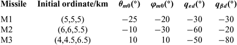
stand for the expected line-of-sight dip angle and line-of-sight drift angle of the missile respectively. The remaining parameters of the three missiles are shown in Table 1.
$q_{\beta d}$
stand for the expected line-of-sight dip angle and line-of-sight drift angle of the missile respectively. The remaining parameters of the three missiles are shown in Table 1.
Table 1. Initial parameters and expected angle
The parameters in the guidance law Equation (11) are set as following:
 $a_{1} =a_{3} =3$
,
$a_{1} =a_{3} =3$
,
 $a_{2} =a_{4} =1.1$
,
$a_{2} =a_{4} =1.1$
,
 ${k}_{1}=k_{2}=k_{3}=k_{4}=1$
,
${k}_{1}=k_{2}=k_{3}=k_{4}=1$
,
 $\alpha _{1} =\alpha _{2} =500$
,
$\alpha _{1} =\alpha _{2} =500$
,
 $\beta _{1} =\beta _{2} =600$
,
$\beta _{1} =\beta _{2} =600$
,
 $\gamma =2.1$
,
$\gamma =2.1$
,
 $u=2.1$
. The parameters of observer Equations (12) and (13) are as following:
$u=2.1$
. The parameters of observer Equations (12) and (13) are as following:
 $\lambda _{0j} =1.1$
,
$\lambda _{0j} =1.1$
,
 $\lambda _{1j} =1.5$
,
$\lambda _{1j} =1.5$
,
 $\lambda _{2j} =2$
;
$\lambda _{2j} =2$
;
 $u_{0j} =3$
,
$u_{0j} =3$
,
 $u_{1j} =6,u_{2j} =8$
,
$u_{1j} =6,u_{2j} =8$
,
 $j=\theta ,\varphi $
;
$j=\theta ,\varphi $
;
 $\text{L}= 0.1$
. The guidance blind area is set to 20m,which means that the missile flies at the acceleration at which it enters the guidance blind area when missile-target distance is less than 20m. The restriction of overload of missile is 30g. The simulation step size is set to 1ms. The simulation results are shown in Fig. 2 and Table 2.
$\text{L}= 0.1$
. The guidance blind area is set to 20m,which means that the missile flies at the acceleration at which it enters the guidance blind area when missile-target distance is less than 20m. The restriction of overload of missile is 30g. The simulation step size is set to 1ms. The simulation results are shown in Fig. 2 and Table 2.

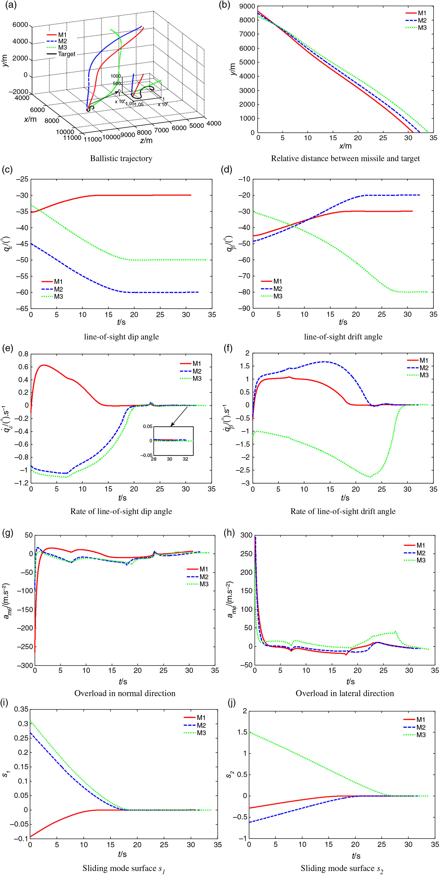
Figure 2. Simulation results of three missiles attacking targets.
Table 2. Simulation results of three missiles attacking targets
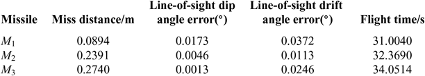
From Table 2 and Fig. 2(a)–(d), it can be known that under the guidance law Equation (11), all three missiles in different states and at different initial positions can hit the maneuvering targets at a specified line-of-sight dip angle and line-of-sight drift angle. The maximum miss distances of the three missiles are no more than 0.3m, errors of line-of-sight dip angle and line-of-sight drift angle are controlled in the range of 0.04
 ${}^\circ$
, which verify the control ability of the guidance law proposed in this paper to control miss distance and impact-angle error. From Fig. 2(e)–(f), It can be known that rates of line-of-sight dip angle and line-of-sight drift angle converge to 0 in finite time, which ensures that the missile can hit the target within a limited time. From Fig. 2(g)–(h), both the overload of missile in normal direction and in lateral direction converge to near 0 at the end of guidance and the convergence process is smooth and chattering free, which ensures the stability of missile control. From Fig. 2(i)–(j), the sliding mode surface
${}^\circ$
, which verify the control ability of the guidance law proposed in this paper to control miss distance and impact-angle error. From Fig. 2(e)–(f), It can be known that rates of line-of-sight dip angle and line-of-sight drift angle converge to 0 in finite time, which ensures that the missile can hit the target within a limited time. From Fig. 2(g)–(h), both the overload of missile in normal direction and in lateral direction converge to near 0 at the end of guidance and the convergence process is smooth and chattering free, which ensures the stability of missile control. From Fig. 2(i)–(j), the sliding mode surface
 ${s}_{1}$
and
${s}_{1}$
and
 ${s}_{2}$
converge to 0 smoothly and continuously in finite time, and the convergence process is chattering free, which proves that the guidance law proposed in this paper can effectively suppress the chattering phenomenon.
${s}_{2}$
converge to 0 smoothly and continuously in finite time, and the convergence process is chattering free, which proves that the guidance law proposed in this paper can effectively suppress the chattering phenomenon.
5.2 Simulation comparison of different guidance laws
In order to further demonstrate the superiority of the guidance law in this paper, mark the guidance law proposed in this paper as SO-NFTSMG, Simulation comparisons is made between it and standard nonsingular sliding mode guidance law (marked as NTSMG1) and first-order sliding mode guidance law (marked as NTSMG2) based on non-singular terminal sliding mode surface and fast power reaching law in Ref. 17.
Now, extend two types of guidance laws to 3D space. The expression of NTSMG1 in 3D space is:
 \begin{equation}
\left\{\begin{split}
a_{m\theta } &=-2\dot{r} x_{2} +\frac{r}{a_{2} k_{2} } sig\left(x_{2} \right)^{2-a_{2} } +K_{1} sgn\left(s_{1} \right) \\
a_{m\varphi } &=\left(2\dot{r} x_{4} -\frac{r}{a_{4} k_{4} } sig\left(x_{4} \right)^{2-a_{4} } +K_{2} sgn\left(s_{2} \right)\right)\cos q_{\varepsilon } \end{split}\right.
\end{equation}
\begin{equation}
\left\{\begin{split}
a_{m\theta } &=-2\dot{r} x_{2} +\frac{r}{a_{2} k_{2} } sig\left(x_{2} \right)^{2-a_{2} } +K_{1} sgn\left(s_{1} \right) \\
a_{m\varphi } &=\left(2\dot{r} x_{4} -\frac{r}{a_{4} k_{4} } sig\left(x_{4} \right)^{2-a_{4} } +K_{2} sgn\left(s_{2} \right)\right)\cos q_{\varepsilon } \end{split}\right.
\end{equation}
Where,
 ${K}_{1}$
and
${K}_{1}$
and
 ${K}_{2}$
are the gain of sign function, according to the upper bound for target maneuvering, In the simulation of this paper, they are selected as 50 and 100, respectively. The remaining parameters in the Equation (29) are selected the same as those of guidance law (Reference Zhao, Li and Liu11).
${K}_{2}$
are the gain of sign function, according to the upper bound for target maneuvering, In the simulation of this paper, they are selected as 50 and 100, respectively. The remaining parameters in the Equation (29) are selected the same as those of guidance law (Reference Zhao, Li and Liu11).
The expression of NTSMG2 in 3D space is:
 \begin{equation}
\left\{\begin{split}
a_{m\theta } &=-2\dot{r} x_{2} +\frac{r}{a_{2} k_{2} } sig\left(x_{2} \right)^{2-a_{2} } +\alpha _{1} sig(s_{1} )^{1-\frac{1}{y} } +\beta _{1} s_{1} \\ a_{m\varphi } &=\left(2\dot{r} x_{4} -\frac{r}{a_{4} k_{4} } sig\left(x_{4} \right)^{2-a_{4} } +\alpha _{2} sig(s_{2} )^{1-\frac{1}{u} } +\beta _{2} s_{2} \right)\cos q_{\varepsilon } \end{split}\right.
\end{equation}
\begin{equation}
\left\{\begin{split}
a_{m\theta } &=-2\dot{r} x_{2} +\frac{r}{a_{2} k_{2} } sig\left(x_{2} \right)^{2-a_{2} } +\alpha _{1} sig(s_{1} )^{1-\frac{1}{y} } +\beta _{1} s_{1} \\ a_{m\varphi } &=\left(2\dot{r} x_{4} -\frac{r}{a_{4} k_{4} } sig\left(x_{4} \right)^{2-a_{4} } +\alpha _{2} sig(s_{2} )^{1-\frac{1}{u} } +\beta _{2} s_{2} \right)\cos q_{\varepsilon } \end{split}\right.
\end{equation}
The parameters in the Eq are selected the same as those of guidance law (Reference Zhao, Li and Liu11).
In the simulation, the missile M1 in Section 5.1. are selected to attack maneuvering targets under the action of SO-NFTSMG, NTSMG1 and NTSMG2 respectively. The initial value of the target and the parameter in the guidance law are the same as those in Section 5.1. Simulation results are shown in Fig. 3 and Table 3.

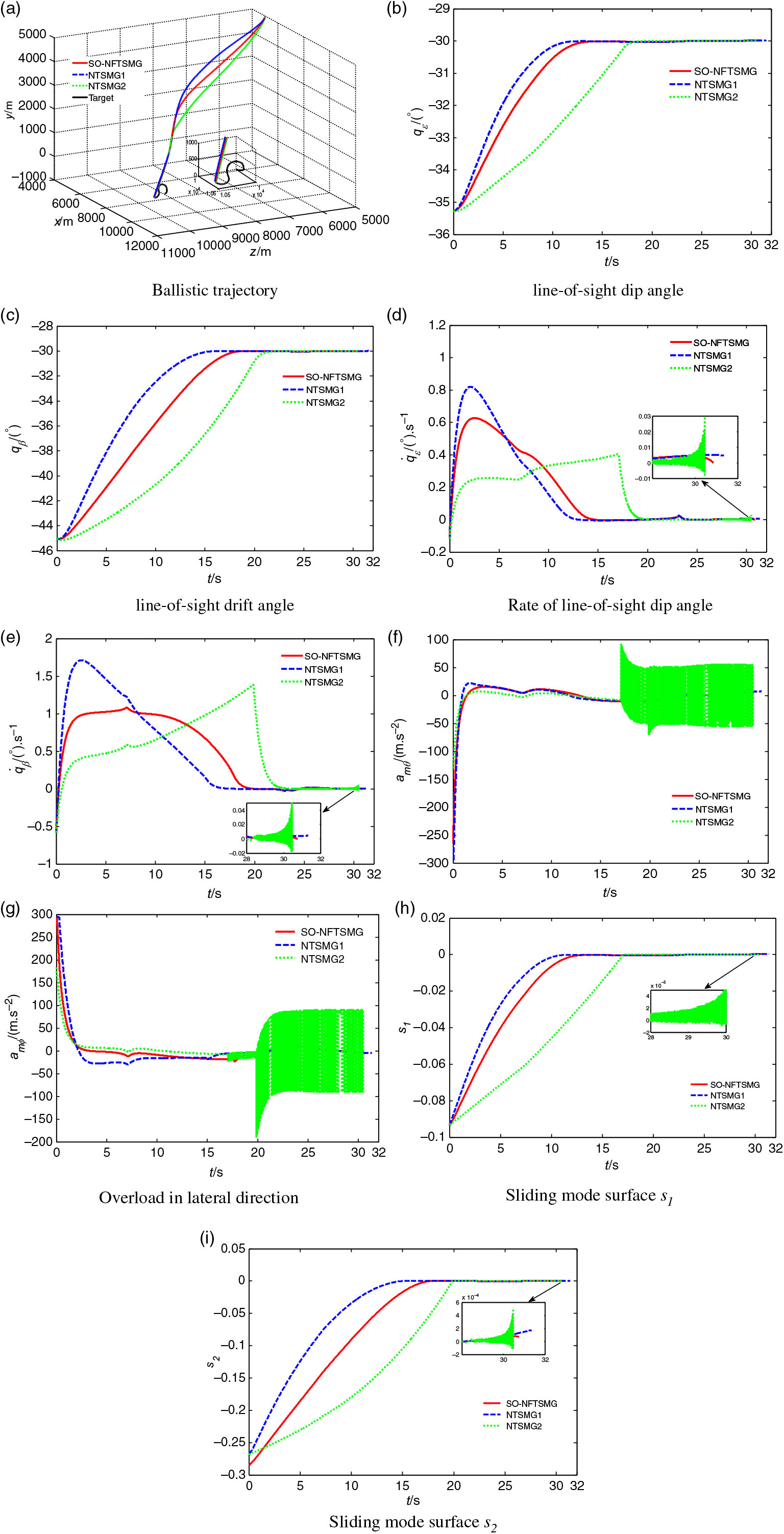
Figure 3. Law simulation results of three guidance laws.
Table 3. Simulation results of three guidance laws
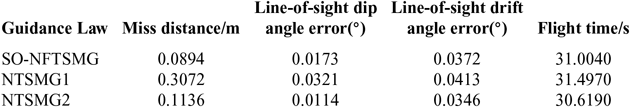
As can be seen from Fig. 3, all three guidance laws can control the missile to hit the maneuvering target at a specified angle. Among them, the convergence speed of SO-NFTSMG and NTSMG1 is relatively fast and similar, and the convergence process is smooth and chattering free. The convergence speed of NTSMG2 is slow, and the phenomenon of high frequency chattering appears in the convergence process, which is not conducive to the control of missile autopilot. From Table 3, it can be seen that the miss distance of missile under action of SO-NFTSMG is the smallest, the line-of-sight dip angle error and line-of-sight drift angle error are smaller than NTSMG1, and the flight time of missile is 0.493s shorter than that of NTSMG1, which increases the penetration probability for the terminal guidance period of missile with shorter flight time. Although the flight time of the missile under action of NTSMG2 is the shortest, and the control ability of miss distance and impact-angle is not much different from that of SO-NFTSMG, the high frequency chattering occurs in the acceleration instruction of NTSMG2, which reduces the control ability of the missile in practical application. The chattering phenomenon cannot be eliminated by substituting the saturation function for the sign function in practical application, and the performance of guidance law will be decreased. Generally speaking, the proposed guidance law SO-NFTSMG has fast convergence speed, stronger ability to control miss distance and impact-angle than NTSMG1, shorter flight time of the missile than that under the action of NTSMG1, and no chattering phenomenon in the guidance command, which is beneficial to the control of missile autopilot.
6.0 CONCLUSION
Based on the theory of the non-singular fast terminal sliding mode surface and the second-order sliding mode control, a new second-order sliding mode three-dimensional guidance law of the non-singular fast terminal with impact-angle constraints is proposed in this paper. There is no need to decouple the model of guidance system and this guidance law can be applied to attack ground maneuvering targets. Aiming at the total disturbance caused by the coupling of target maneuvering information and line-of-sight angle, we design the nonhomogeneous disturbance observer to estimate and prior information of target is not needed. The results of two groups of experiment simulation show that the guidance law proposed in this paper can control multiple missiles at different positions and different states to hit the target at their expected angles, with fast convergence speed, short flight time, strong ability to control miss distance and impact-angle and no chattering phenomena appear during the process of convergence, which make it has practical application value. However, it is still worth further study to consider the dynamic characteristics of autopilot and how to reduce the required information.