


NOMENCLATURE
- ax, ay, az
Body axes accelerations, m/s2
- CD, CL, CY
Drag, lift and side force aerodynamic coefficients
 ${{\rm C}}_{{{\rm D}}_0},{{\rm C}}_{{{\rm L}}_0}, { \ }{{\rm C}}_{{{\rm Y}}_0}$
Non-dimensional parameter constants of lift, drag and side force at zero angle-of-attack
- ${{\rm C}}_{{{\rm L}}_{(.)}},{{\rm C}}_{{{\rm Y}}_{(.)}}{\rm ,\ }{{\rm C}}_{{{\rm D}}_{(.)}}$
Non-dimensional derivative of lift, side and drag force coefficients
- Cl, Cm, Cn
Rolling, pitching and yawing moment coefficients
- ${{{\rm C}}_{{{\rm l}}_0}{\rm ,C}}_{{{\rm m}}_0},{{\rm C}}_{{{\rm n}}_0}$
Non-dimensional constant of rolling, pitching and yawing moment at zero angle-of-attack
- ${{{\rm C}}_{{{\rm l}}_{(.)}}{\rm ,C}}_{{{\rm m}}_{(.)}},{{\rm C}}_{{{\rm n}}_{(.)}}$
Non-dimensional derivative of rolling, pitching and yawing moment coefficients
- α, β
Free stream angle-of-attack and sideslip angle, degree
- x, y, z
Position variable of UAV w.r.t inertial frame, m
- Φ, θ, ψ
Euler angles of UAV w.r.t inertial frame, degree
- u, v, w
Body axes velocity components of UAV, m/s
- p, q, r
Body axes Euler rates (roll, pitch and yaw), rad/s
- δ a, δ e, δ r
Aileron, elevator and rudder deflection angles, degree
- Ix, Iy, Iz
Body axes moment of inertia components along x-y-z axis, kg-m2
- Ixz
Cross moment of inertia components in x-z plane, kg-m2
- $\widehat{{\rm c}}$
Mean aerodynamic chord, m
- g
Acceleration due to gravity, m/s2
- k
Correction factor in induced drag
- m
Mass of UAV, kg
- S
Reference wing area, m2
- J
Cost function
- T
Thrust, N
- V
Free stream velocity, m/s
- Z
Measured Flight flight Datadata
- ρ
Free stream density, kg/m3
- Θ
Vector of Aerodynamic aerodynamic parameters to be estimated
- λ
Taper ratio
- ${(^{\cdot})}$
Time derivative


1.0 INTRODUCTION
Unmanned aerial vehicles (UAVs) are playing an increasingly important role in both civilian and military operations. This remarkable development of UAVs is largely due the operational ease, cost-effectiveness and increased control capabilities in the field with its unmanned flight. Common military applications of UAV include reconnaissance, surveillance, combat, rescue, battle damage assessment and communications relays. Design of UAV is quite robust in its development and presents vast research opportunities(Reference Keane, Scanlan and Bressloff1), depending upon mission requirements or selection of design and configuration. These design considerations are based on aerodynamic characteristics, performance evaluation, stability-control analysis, simulation and structural stress analysis. Traditionally analytical methods, wind-tunnel testing, Computational fluid dynamics (CFD) analysis and flight tests are used to develop the aerodynamic database for designing the most efficient autonomous flight controllers. A database of aerodynamic parameters, which characterise the performance of the flight vehicle, helps in the diagnosis of the design of the UAV and its autonomous capability.
Theoretical estimates of aerodynamic parameters depend upon historical database and analytical expressions, which are less accurate and need to be verified with experiments. The generated aerodynamic database from wind-tunnel tests needs corrections such as wall/sting interference, scale factor, and Reynold’s number duplication, etc. to name a few. Experimental measurements or CFD analyses are limited to the estimation of static aerodynamic parameters and are complementary during preliminary design phase(Reference Murphy2). Parameter estimation from flight data not only addresses the aforementioned issues, but it also enhances the accuracy and comprehensiveness of the aerodynamic model structure of the flight vehicle. Estimation of parameters for small UAVs is a research area of constant exploration(Reference Maine and Iliff3). Constrained parameter optimisation algorithm is traditionally used to estimate aerodynamic parameters from the flight tests of a conventional fixed-wing UAV. Suk et al details a comparison of performance for extended Kalman filter (EKF), simplified and augmented versions of unscented Kalman filter (UKF) methods in time domain for estimating the parameters from the flight data of fixed-wing aircraft (HFB-320) and a rotary-wing UAV (ARTIS)(Reference Suk, Lee, Kim, Koo and Kim4,Reference Chowdhary and Jategaonkar5) . Condomines et al uses UKF technique to estimate wind field and aerodynamic parameters of a small-scale glider UAV (Solius glider)(Reference Condomines, Bronz and Hattenberger6). Meng et al extends the application of iterated EKF technique to estimate the parameters from simulated non-linear flight data of a small fixed-wing UAV(Reference Meng, Li and Veres7). Dorobantu et al identifies aerodynamic parameters of a low-cost, fixed-wing UAV (Ultra Stick 25e) by fitting the model to frequency responses extracted from the flight data(Reference Dorobantu, Murch, Mettler and Balas8). Padayachee et al discusses the regression analysis and maximum likelihood (ML) method to perform aerodynamic model identification of a twin-boom electrically powered fixed-wing UAV from flight data(Reference Padayachee9). Chase et al demonstrates estimation of longitudinal aerodynamic force coefficients using least squares (LS) and Kalman Filter regression models from flight tests of fixed-wing UAV(Reference Chase and McDonald10). Hoffer et al elaborates on recursive least squares algorithm with error filtering–based online learning scheme to develop the aerodynamic model of a low-cost fixed-wing T-tail UAV(Reference Hoffer, Coopmans, Fullmer and Chen11). Jameson et al addresses the effects of reconstruction and differentiation of state variables on the reliability of estimated parameters, using simulated flight data of Aerosonde UAV (fixed-wing twin-tail-boom UAV)(Reference Jameson and Cooke12). Tieying et al proposed modified particle swarm optimisation methodology to carry out the longitudinal parameter identification of a small UAV from flight tests(Reference Tieying, Jiei and Kewei13). Hemakumara et al proposed non-parametric approach based on multi-output local and global Gaussian process approximations to estimate the parameters from flight tests of a fixed-wing UAV (Brumby Mk-III UAV) with canard configuration(Reference Hemakumara and Sukkarieh14).
Majority of the system identification research on UAVs has been carried out using classical estimation techniques such as ML, LS and Kalman filter methods. Fixed-wing UAVs considered for parameter identification research correspond only to conventional configurations. Black-box estimation methods based on artificial neural networks (ANNs) have also been successfully used for the identification problems for both fixed- and rotary-wing aircrafts and are gaining acceptability in research and industry(Reference Ben Mosbah, Botez and Dao15–Reference Tischler and Remple19). Peyada et al proposed a neural Gauss–Newton (NGN) method for parameter estimation of flight vehicles that are validated for low angles of attack flight data of manned (Hansa-3 and ATTAS) aircrafts(Reference Peyada and Ghosh20,Reference Peyada and Ghosh21) .
This work extends the application of LS, Maximum Likelihood Estimation (MLE) and NGN methods for parameter estimation for unconventional UAV from the longitudinal and lateral-directional flight tests data, with flow angles measured explicitly. This paper presents a full-scale wind-tunnel test of Cropped Delta Reflex Wing configuration to analyse the aerodynamic model structure that needs to be postulated a priori for parameter estimation from flight data. The estimated responses of the motion variables using NGN method are compared with the classical ML and LS methods for their longitudinal and lateral/directional dynamics. Confidence levels in the estimated parameters were quantified by means of respective Cramer-Rao bounds(Reference Murphy2). To examine the consistency of estimates from the three methods, a scatter plot, along with the mean and standard deviation, is presented. Finally, the estimates and the aerodynamic model are validated by means of a proof-of-match exercise.
2.0 UAV DYNAMICS
This section presents a brief description of the aircraft longitudinal and lateral-directional dynamics of the CDRW UAV. Rigid-body equations of motion are used to define the kinetics of the UAV. Although coupled six degrees of freedom (DOF) equations are required to define the complete dynamics of UAV, Equations (1)–(4) and Equations (5)–(8) are used during the simulation of CDRW, with the assumption that the longitudinal controls/disturbance will not affect the lateral-directional dynamics and vice versa(Reference Jategaonkar22).
 \begin{equation}\dot{V}=\frac{\rho sV^{2}}{2m}C_D+\frac{T}{m}{cos \alpha \ }+g{sin \left(\theta -\alpha \right)\ }\end{equation}
 \begin{equation}\dot{\alpha }=-\frac{\rho sV}{2m}C_L+q-\frac{T}{mV}{sin \alpha \ }+\frac{g}{V}{cos \left(\theta -\alpha \right)\ }\end{equation}
 \begin{equation}\dot{q}=\frac{\rho sV^{2}\hat{c}}{2I_y}C_m+M_{Thrust}\end{equation}
 \begin{equation} \dot{\theta }=q \end{equation}
 \begin{equation} \dot{\beta }=-\frac{\rho sV}{2m}C_Y-r+\frac{T}{mV}{sin \beta \ }+\frac{g}{V}{sin \left(\theta -\alpha \right)\ }\end{equation}
 \begin{equation} \dot{p}=\left(\frac{1}{J_{xx}J_{zz}-{\ }J^{2}_{xz}}\right)\left\{J_{zz}{ \ }L{ +\ }J_{xz}{ \ }N\right\}\end{equation}
 \begin{equation} \dot{r}=\left(\frac{1}{J_{xx}J_{zz}-{\ }J^{2}_{xz}}\right)\left\{J_{xz}{ \ }L{ +\ }J_{xx}{ \ }N\right\}\end{equation}
 \begin{equation} \dot{\phi}=p \end{equation}
where  $V=\sqrt{u^2+v^2+w^2}$ is the true airspeed, α is the angle-of-attack, β is the sideslip angle, θ is the pitch angle, φ is the roll angle, p is the roll rate, q is the pitch rate, r is the yaw rate, T is the thrust input, ρ is the air density, s is the wing surface area, b is the span of the wing and
  $\hat{c}$ is the length of the wing chord. I x denotes the moment of inertia along x-axis, I y is the moment of inertia along y-axis, I z is the moment of inertia along z-axis and I xz is the cross-coupled moment of inertia about x-z plane. M Thrust is the moment created by the engine thrust, and the variables obtained from the longitudinal motion model are considered as pseudo control variables.
The aerodynamic force and moment coefficients appearing in Equations (1)–(8) are modelled as follows(Reference Jategaonkar22):
 \begin{equation} C_L=C_{L_0}+C_{L_{\alpha }}\alpha +C_{L_q}\left(\frac{q\hat{c}}{2V}\right)+C_{L_{{\delta }_e}}{\delta }_e \end{equation}
 \begin{equation} C_D=C_{D_0}+kC^{2}_L \end{equation}
 \begin{equation} C_m=C_{m_0}+C_{m_{\alpha }}\alpha +C_{m_q}\left(\frac{q\hat{c}}{2V}\right)+C_{m_{{\delta }_e}}{\delta }_e \end{equation}
 \begin{equation} C_Y=C_{Y_0}+C_{Y_{\beta }}\beta +C_{Y_r}\left(\frac{rb}{2V}\right)+C_{Y_p}\left(\frac{pb}{2V}\right)+C_{Y_{{\delta }_r}}{\delta }_r+C_{Y_{{\delta }_a}}{\delta }_a \end{equation}
 \begin{equation} C_l=C_{l_0}+C_{l_{\beta }}\beta +C_{l_r}\left(\frac{rb}{2V}\right)+C_{l_p}\left(\frac{pb}{2V}\right)+C_{l_{{\delta }_r}}{\delta }_r+C_{l_{{\delta }_a}}{\delta }_a \end{equation}
 \begin{equation} C_n=C_{n_0}+C_{n_{\beta }}\beta +C_{n_r}\left(\frac{rb}{2V}\right)+C_{n_p}\left(\frac{pb}{2V}\right)+C_{n_{{\delta }_r}}{\delta }_r+C_{n_{{\delta }_a}}{\delta }_a \end{equation}
where δ e is elevator deflection, δ r is rudder deflection and δ a is aileron deflection. Induced drag correction factor k, in Equation (10), is taken as an input from wind-tunnel measurements, with a considered value of 0.12.
The vectors ΘLG in Equation (15) and ΘLD in Equation (16) consist of the set of longitudinal and lateral-directional parameters, respectively, that are to be estimated
 \begin{equation} {\Theta }_{LG}={\left[C_{L_0}{ \ }C_{L_{\alpha }}{ \ }C_{L_q}{ \ }C_{L_{{\delta }_e}}{ \ }C_{D_0}{ \ }C_{m_0}{ \ }C_{m_{\alpha }}{ \ }C_{m_q}{ \ }C_{m_{{\delta }_e}}\right]}^T \end{equation}
 \begin{equation} {\Theta }_{LD}={\left[C_{Y_0}{ \ }C_{Y_{\beta }}{ \ }C_{Y_r}{ \ }C_{Y_p}{ \ }C_{Y_{{\delta }_r}}{ \ }C_{l_0}{ \ }C_{l_{\beta }}{ \ }C_{l_r}{ \ }C_{l_p}{ \ }C_{l_{{\delta }_r}}{ \ }C_{l_{{\delta }_a}}{ \ }C_{n_0}{ \ }C_{n_{\beta }}{ \ }C_{n_r}{ \ }C_{n_p}{ \ }C_{n_{{\delta }_r}}\right]}^T \end{equation}
where  $C_{Y_{{\delta }_a}},\ C_{n_{{\delta }_a}}$ are identified to be negligible from wind-tunnel data and hence are not considered during the process of parameter estimation.
3.0 PARAMETER ESTIMATION METHODS
This subsection describes the estimation techniques, namely ML, LS and NGN methods, used for longitudinal and lateral-directional aerodynamic characterisation of CDRW UAV from flight data. For the estimation of parameters using LS and NGN methods, the non-dimensional aerodynamic force and moment coefficients are required as an input. Since these aerodynamic coefficients cannot be measured directly during flight test, Equations (17)–(24), which are a function of measured variables, are used to obtain the aforesaid coefficients(Reference Kumar and Ghosh23).
 \begin{equation} C_X(k)=\left(ma_{X_{CG}}(k)-T\right){ /}\hat{q}(k)S\end{equation}
 \begin{equation} C_Z(k)=ma_{Z_{CG}}(k){ /}\hat{q}(k)S\end{equation}
 \begin{equation} C_L(k)=C_X(k){sin \alpha \ }(k)-C_z(k){cos \alpha \ }(k)\end{equation}
 \begin{equation} C_D(k)=-C_X(k){cos \alpha \ }(k)-C_Z(k){sin \alpha \ }(k)\end{equation}
 \begin{equation} C_m(k)=\left[I_y\dot{q}(k)-I_{xz}\left(p^{2}(k)-r^{2}(k)\right)-\left(I_z-I_X\right)p(k)r(k)\right]{ /}\left(\hat{q}(k)\hat{c}S\right)\end{equation}
 \begin{equation} C_Y(k)=ma_{Y_{CG}}(k){ /}\hat{q}(k)S \end{equation}
 \begin{equation} C_l(k)=\left[I_x\dot{p}(k)-I_{yz}(q^{2}(k)-r^{2}(k))+(I_z-I_y)r(k)q(k)\right]{ /}\left(\hat{q}(k)bS\right)\end{equation}
 \begin{equation} C_n(k)=\left[I_z\dot{r}(k)+I_{xy}(q^{2}(k)-p^{2}(k))+(I_y-I_x)p(k)q(k)\right]{ /}\left(\hat{q}(k)bS\right)\end{equation}
where  $a_{X_{CG}},\ a_{Y_{CG}},\ a_{Z_{CG}}$ denote the net accelerations along x, y and z axes in body frame; C X, C Y, C Z are the force aerodynamic coefficients along x, y and z axes in body frame; C L, C D, C Y are the lift, drag and yawing force aerodynamic coefficients derived using C X, C Y, C Z and C l, C m, C n are the roll, pitch and yawing moment aerodynamic coefficients along x, y and z axes.
3.1 Least square method
The LS estimation is a classical methodology(Reference Murphy2) that belongs to a class of equation error methods. The LS method is not necessarily based on any statistical formulation but is often characterised in statistical terms as estimates, denoted by random variables formulation. It is denoted by the form:
 \begin{equation} Y=X\Theta { +\ }\varepsilon \end{equation}
where, Y is a N vector of response variable for data measurement points, X is an N × n matrix of the state and input variables,  $\Theta $ is a n vector of unknown parameters and
  $\varepsilon $ is the error in modelling. The LS solution will lead to the exact estimates of unknown parameters in the absence of both measurement and process noise. The estimates determined using the LS method solely depends on the cause–effect relationship in terms of dependent and independent variables. Performance of the LS method also depends on the quality of data generated, and it is assumed that independent variables are noise free, and dependent variables are corrupted by a uniformly distributed noise. The LS solution of the unknown parameters (
 $\Theta $) is estimated by minimising the following cost function:
 \begin{equation} J{\left(\Theta \right)}_{LS}=\frac{1}{2}{\varepsilon }^T\varepsilon =\frac{1}{2}\left[Y^T-{\Theta }^TX^T\right]\left[Y-X\Theta \right] \end{equation}
where Y and X are vectors of dependent and independent variables, respectively, and  $\varepsilon$ is the error in modelling(Reference Jategaonkar22). The solution to the LS estimate is given as:
 \begin{equation} \widehat{\Theta }={(X^TX)}^{-1}X^TY \end{equation}
3.2 Maximum likelihood method
Output error estimation method based on the ML function is a time-domain batch methodology, which is used to estimate aerodynamic parameters of aircrafts from flight tests(Reference Maine and Iliff3,Reference Jategaonkar22,Reference Mehra, Stepner and Tyler24) . The ML estimator requires a priori mathematical postulation of the flight dynamics accompanied by an accurate aerodynamic model, which is either a linear or a nonlinear function of aerodynamic parameters. The ML-based methods are effectively used for aircraft parameter estimation problems, even in the presence of noise in the measured flight data. The system is corrupted by measurement noise, which is statistically independent and identically distributed. In the presence of process noise, efficiency of ML estimates degrades due to convergence problems. Desired control input for a manoeuvre is independent of systems response and should sufficiently excite various modes of flight. The output vector of N observations, which depends on the unknown parameter vector  $\Theta $, comprises aerodynamic parameters, initial conditions, measurement noise and process noise. Considering the measurements to be fixed, probability density function is represented by a single parameter
  $\Theta $, referred to as the likelihood function. ML method is defined as the study for which the outcome of the experiment is most likely or the probability density function is maximised w.r.t
  $\Theta $. The parameters are estimated by maximising the likelihood function representing the probability density of observed variables. Therefore, the problem of finding a maximum likelihood estimate becomes the problem of finding the
  $\Theta $ that maximises the likelihood function. The ML algorithm requires the initial guess values of unknown parameters as an input, which are subsequently optimised by means of Gauss-Newton algorithm. Cost function is defined as(Reference Jategaonkar22,Reference Mehra, Stepner and Tyler24)
 \begin{equation} J\left(\Theta \right)=\left(\frac{1}{2}\right)\sum^N_{i=1}{\left\{{\left[Z\left(t_i\right)-Y_{\Theta }\left(t_i\right)\right]}^T{\left(GG^T\right)}^{-1}\left[Z\left(t_i\right)-Y_{\Theta }\left(t_i\right)\right]\right\}} \end{equation}
where N is the length of data recorded, GGT is the covariance of measurement noise and  $Y_{\Theta }\left(t_i\right)$ is the simulated response with given initial conditions and the guess values of unknown aerodynamic parameters,
  $\Theta $.
3.3 Neural Gauss-Newton method
The NGN is one of the recent methodologies for parameter estimation, based on ANNs, that has been applied to estimate both longitudinal and lateral-directional parameters of the current UAV. The NGN estimation method is a time-domain post-processing technique that utilises a feedforward neural network (FFNN) for a neural model utilised to predict the subsequent behaviour of the flight vehicle over a period of time for given initial conditions(Reference Peyada and Ghosh20–Reference Jategaonkar22,Reference Kumar25,Reference Dhayalan26) . The NGN training model is a point-to-point mapping of the input and output data to represent the flight dynamic model. The usage of neural model circumvents the need to use a definitive mathematical description of the flight dynamics, thereby bypassing the numerical integration of equations of motion. This particular feature enables the NGN method to handle the process noise in the mathematical model. This neural model comprise of measured compatible flight data of the motion and control variables. This validated neural model, which is obtained post training, is used to compute response for any arbitrary control input within the training boundary. This trained neural model is used to predict subsequent motion variables at (k + 1) th instant for given measured initial variables at k th instant (where k = 1 to n: n is the length of the data record). This approach is used to build flight dynamic model, in a limited sense, from measured data for a given range of training boundary.
The schematic of the neural architecture used during the training of longitudinal and lateral-directional flight dynamic model of CDRW is presented in Fig. 1. Following vectors U(k) and Z(k+1) in Equations (29) and (30), respectively, represent the input and output vectors for neural training process
 \begin{equation} U_k={\left[V_k{\rm ,\ }{\alpha }_k{\rm ,\ }{\beta }_k{\rm ,\ }{\Phi }_k{\rm ,\ }{\theta }_k{\rm ,\ }{\Psi }_k{\rm ,\ }p_k{\rm ,\ }q_k{\rm ,\ }r_k{\rm ,\ }{C_D}_k{\rm ,\ }{C_Y}_k,{C_L}_k{\rm ,\ }{C_l}_k,{C_m}_k{\rm ,\ }{C_n}_k\right]}^T \end{equation}
 \begin{align}Z_{k+1}&=\left[V_{k+1}{\rm ,\ }{\alpha }_{k+1}{\rm ,\ }{\beta }_{k+1}{\rm ,\ }{\Phi }_{k+1}{\rm ,\ }{\theta }_{k+1}{\rm ,\ }{\Psi }_{k+1}{\rm ,\ }p_{k+1}{\rm ,\ }q_{k+1}{\rm ,\ }r_{k{\rm +!}}{\rm ,\ }{C_D}_{k+1}{\rm ,\ }\right.\nonumber\\
&\quad\left.{C_Y}_{k+1},{C_L}_{k+1}{\rm ,\ }{C_l}_{k+1},{C_m}_{k+1}{\rm ,\ }{C_n}_{k+1}\right]^T \end{align}
\begin{align}Z_{k+1}&=\left[V_{k+1}{\rm ,\ }{\alpha }_{k+1}{\rm ,\ }{\beta }_{k+1}{\rm ,\ }{\Phi }_{k+1}{\rm ,\ }{\theta }_{k+1}{\rm ,\ }{\Psi }_{k+1}{\rm ,\ }p_{k+1}{\rm ,\ }q_{k+1}{\rm ,\ }r_{k{\rm +!}}{\rm ,\ }{C_D}_{k+1}{\rm ,\ }\right.\nonumber\\
&\quad\left.{C_Y}_{k+1},{C_L}_{k+1}{\rm ,\ }{C_l}_{k+1},{C_m}_{k+1}{\rm ,\ }{C_n}_{k+1}\right]^T \end{align}
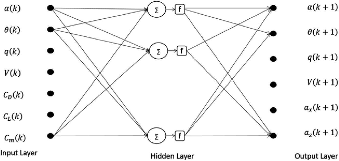
Figure 1. Neural architecture for building restricted flight dynamic model(Reference Dhayalan26).
The quality of the acquired flight data influences the performance and applicability of the neural model. Tuning of these parameters requires proper attention to avoid over- or undertraining of the neural network. Careful selection of number of neuron in hidden layer as well as iterations also plays a significant role while handling measured data corrupted by noise(Reference Ben Mosbah, Botez and Dao15–Reference Boëly, Botez and Kouba17,Reference Kumar, Ganguli, Omkar and Kumar27) . This trained neural model predicts the system output ( $Y_{\Theta }$) corresponding to assumed aerodynamic model and with measured initial conditions as an input. The initial guess parameters are then optimised using Gauss-Newton algorithm, minimising the error cost function(Reference Peyada and Ghosh21,Reference Napolitano28,Reference Saderla29) .
4.0 MODEL SPECIFICATIONS
This section presents the inertial and geometric details of CDRW UAV.
A detailed design methodology adapted to develop CDRW is presented in Ref. (Reference Saderla29). The CDRW is a wing-alone blended-wing configuration with no horizontal stabiliser and a dedicated fuselage. The cross-section of the wing is a NACA 23110 reflex aerofoil. Figure 2 represents the planform view and side view of the designed CDRW configuration. The control surface, called as elevons located aft of the root chord, provide both longitudinal and lateral control. Whereas, the all-movable vertical tail of high aspect ratio provides directional control. The high aspect ratio all movable vertical tail, located aft of the root chord, provides directional stability and control. The cross-section of the dedicated all-movable vertical tail is a symmetric NACA 0012 aerofoil. Geometric and design details of CDRW are presented in Table 1.

Figure 2. Schematic planform view and side view of CDRW UAV(Reference Saderla29).
Table 1 Design, inertial and geometric details of CDRW UAV

5.0 WIND-TUNNEL TESTING
Prior to performing the flight tests, the CDRW model was subjected to full-scale wind-tunnel testing at the National Wind Tunnel Testing Facility (NWTF), IIT Kanpur, to understand as well as to identify the form of static aerodynamic model structure and the respective parameters. The cross-sectional dimensions of this low-speed closed-circuit wind-tunnel test section is  $3.0\ \text{m} \times 2.25\ \text{m}$(Reference Saderla, Rajaram and Ghosh30). The
  $\beta-\text{mechanism}$ of the test section, which is a cantilever structure supported by means of two coaxial turn tables, plays a vital role in the variation of angle-of-attack and sideslip angles during the experiments.
During wind-tunnel tests, the forces and moments acting on the UAV are measured by means of a six-component pre-calibrated load balance. Figure 3 presents the schematic and the photograph of the model mounted on  $\beta-\text{mechanism}$. It can be noticed that the rear-end adapter holds the load balance with the
  $\beta-\text{mechanism}$, whereas the front-end adapter acts as an interface between the load balance and the model. The front-end adapter transfers the aerodynamic loads acting on the model to the balance and houses the balance during the tests.
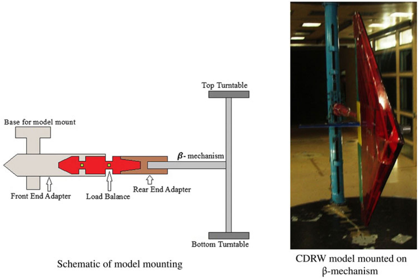
Figure 3. CDRW model mounting in side test section of the NWTF.
Measurements of longitudinal static aerodynamic force and moment coefficients of CDRW UAV were obtained by performing an alpha sweep test in which the angle-of-attack is varied from  $-5^\circ$ to
  $50^\circ$ at a rate of
  $0.1^\circ$ per second. Similarly, sideslip angle is varied from
  $-15^\circ$ to
  $15^\circ$ at a rate of
  $0.1\circ$ per second for determining lateral-directional force and moment coefficients. Through the wind-tunnel tests, it is made consistent that at least three data points are collected between any two consecutive flow angles. Initially, a velocity sweep test from 5 m/s to 35 m/s with an interval of 3 m/s is performed on CDRW configuration. It is observed that this specified range of velocity has no significant effect of Reynolds number on the aerodynamic force and moment coefficients. For all the wind-tunnel experiments, a Reynolds number of
  $3.45 \times 10^{5}$ is maintained, with
  $\hat{c}$ as the characteristic length.
The variation of non-dimensional lift, drag and moment coefficients with angle-of-attack of CDRW UAV from the wind-tunnel tests is presented in Fig. 4. Figure 5 denotes the variation of non-dimensional side-force, rolling and yawing moment coefficients with sideslip angle. During these tests, the span of the model is accommodated along the width of the test section and made parallel to its floor/roof. Longitudinal and lateral-directional stability and control derivatives derived from these wind-tunnel tests have been tabulated in Tables 4, 5 and 6, along with the results from parameter estimation, using flight data.
Figure 4. Generated longitudinal aerodynamic force and moment coefficients of CDRW(Reference Saderla29).

Figure 5. Generated lateral-directional aerodynamic force and moment coefficients of CDRW(Reference Saderla29).
6.0 GENERATION OF FLIGHT DATA
Flight data generation is the process of recording the commanded inputs and the corresponding response of the flight vehicle(Reference Jategaonkar22). Data gathering is one of the crucial aspects of flight vehicle system identification, as the basic rule that applies to any system for parameter estimation from experimental data is ‘If it is not in the data, it cannot be modeled’. This rule is true irrespective of the type of flight vehicle, either manned or unmanned, considered for aerodynamic characterisation. It can be observed that the scope of parameter estimation technique is limited by the quality of the generated flight data. The accuracy and reliability of the estimated parameters depend on the amount of information available in the particular set of flight data, irrespective of using either the classical or neural-based method. Proper instrumentation, precise calibration and appropriate control input design play a vital role in the generation of reliable flight data for parameter estimation. Rigorous flight tests have been performed with the instrumented CDRW configuration in flight laboratory at IIT Kanpur. During flight tests, predecided control inputs were applied in an attempt to excite the appropriate dynamics of the CDRW UAV. These manoeuvres were executed about the trim velocities varying from 18 m/s to 25 m/s and thrust is held constant by holding the throttle stick at a constant position. During the manoeuvres, the respective dynamics of UAV is captured by means of a dedicated onboard data acquisition system, which is capable of on-board logging and data telemetry. Lab-view platform has been used at the ground station to develop a graphical user interface that facilitates real-time visualisation of telemetry data and also for an additional logging of the received data.
The UAV’s motion variables, linear accelerations ( $a_x,a_y,a_z$), body angular rates (p,q,r) and Euler angles (
 $\phi,\theta ,\psi$), are measured by means of a nine-DOF inertial measurement unit attached to the data acquisition system. Thrust and control surface deflections (
 ${\delta }_e,{\delta }_a,{\delta }_r$) are inputs recorded by tapping the pulse-density and pulse-width modulation signals from the speed controller and servos, respectively.
Velocity and altitude of flight are obtained from two sets of measurements, one from pre-calibrated absolute and differential pressure sensors attached to pitot and static tubes and the other from Global positioning system (GPS) unit(Reference Saderla29). The data acquisition system also consists of six analog and digital input ports. Angle-of-attack ( $\alpha $) and angle of sideslip (
 $\beta $) are measured by means of an in-house fabricated multi-turn potentiometer-based vane-type sensors in the form of analog signals. The calibration details of the flow angle sensors, servos and static thrust from the motor are detailed in Ref. (Reference Saderla29).
The instrumented CDRW prototype along with the flight data acquisition system is presented in Fig. 6. Predefined control inputs are executed for the UAV trimmed at an altitude of approximately 50–70 m and is verified in real time from the online display of flight data. Following this approach, various modes of flight were executed during moderately calm weather. A total of 12 sets of flight data were used, with six each for longitudinal and lateral-directional parameter estimation using ML, LS and NGN methods, respectively.
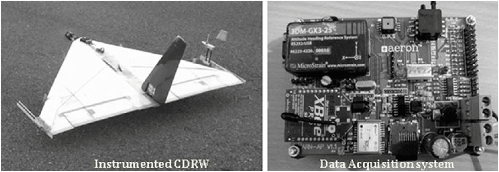
Figure 6. Instrumented CDRW configuration and the data acquisition system for flight tests.
Flight data classification is performed as follows: URW_LG1 to URW_LG6 for longitudinal cases and URW_LD1 to URW_LD6 for lateral directional manoeuvres. URW in the aforementioned flight data nomenclature denotes unmanned reflex wing, and LG and LD denote longitudinal and lateral directional cases, respectively, followed by a numeric for corresponding flight data set.
As mentioned previously, six sets of longitudinal flight data (URW_LG1-URW_LG6) and six sets of lateral-directional flight data (URW_LD1-URW_LD6) are used to carry out the compatibility check. Tables 2 and 3 present the obtained results of compatibility check for longitudinal and lateral-directional flight data. It can be observed that the scale factors  $K_{\alpha }$ and
  $K_{\beta }$ are close to unity, biases are negligible for both the cases and the influence of system errors on the measured motion variables is minimal. The corresponding lower values of Cramer-Rao bounds, obtained as an output of the ML method, further enhanced the confidence level in the acquired flight data of the CDRW configuration. The flight data measured by means of sensors consist of motion variables, which are susceptible to systematic and random errors. These measured data, corrupted with errors, cannot be used directly for parameter estimation, since these introduce data incompatibility. An independent check needs to be performed to verify the consistency of the measured variables. To estimate these errors, a kinematic consistency check was performed by considering the measured accelerations and angular rates as an input. This process of data compatibility check, which is also termed flight path reconstruction (FPR), is as an integral part of aircraft parameter estimation. The primary goal of FPR is to identify the systematic errors and to make the flight data consistent prior to parameter estimation.
Table 2 Data compatibility check for cropped delta reflex-wing longitudinal flight data

Values in parentheses represent Cramer-Rao bound.
Table 3 Data Compatibility check for cropped delta reflex-wing lateral-directional flight data

Values in parentheses represent Cramer-Rao Bound.
A deterministic output error technique is used to estimate the set of unknown parameters in terms of scale factors and biases. Vectors  ${\Theta }_{FPR\_LG}$ and
  ${\Theta }_{FPR\_LD}$ in Equations (31) and (32) represent the systematic errors estimated for longitudinal and lateral-directional cases, respectively.
 \begin{equation} {\Theta }_{FPR\_LG}={\left[\Delta a_x{ \ }\Delta a_y{ \ }\Delta a_z{ \ }\Delta p{ \ }\Delta q{ \ }\Delta r{ \ }K_{\alpha }{ \ }\Delta \alpha \right]}^T\end{equation}
 \begin{equation} {\Theta }_{FPR\_LD}={\left[\Delta a_x{ \ }\Delta a_y{ \ }\Delta a_z{ \ }\Delta p{ \ }\Delta q{ \ }\Delta r{ \ }K_{\beta }{ \ }\Delta \beta \right]}^T\end{equation}
Figures 7 and 8 present the measured and computed response of motion variables ( $V,\ \alpha ,\beta ,\phi,\theta ,\psi $) obtained during the data compatibility check from flight data for longitudinal and lateral-directional control inputs, respectively. It is observed from the figures that most of the reconstructed state variables are a close match with the measured flight data. The flight data were reconstructed after incorporating the centre of gravity shift, biases and scale factors, and the resulting sets of compatible flight data are used to perform aerodynamic characterisation by using parameter estimation methods.
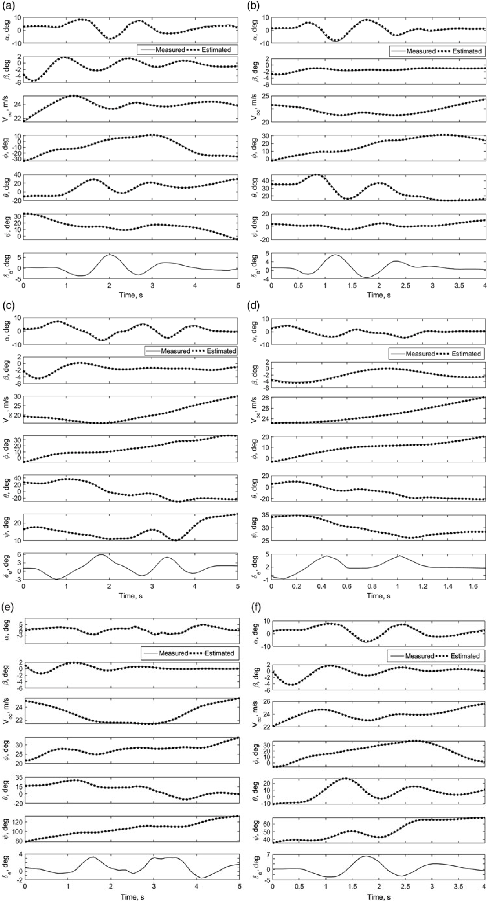
Figure 7. Data compatibility check of CDRW longitudinal configuration: URW_LG1-LG6.
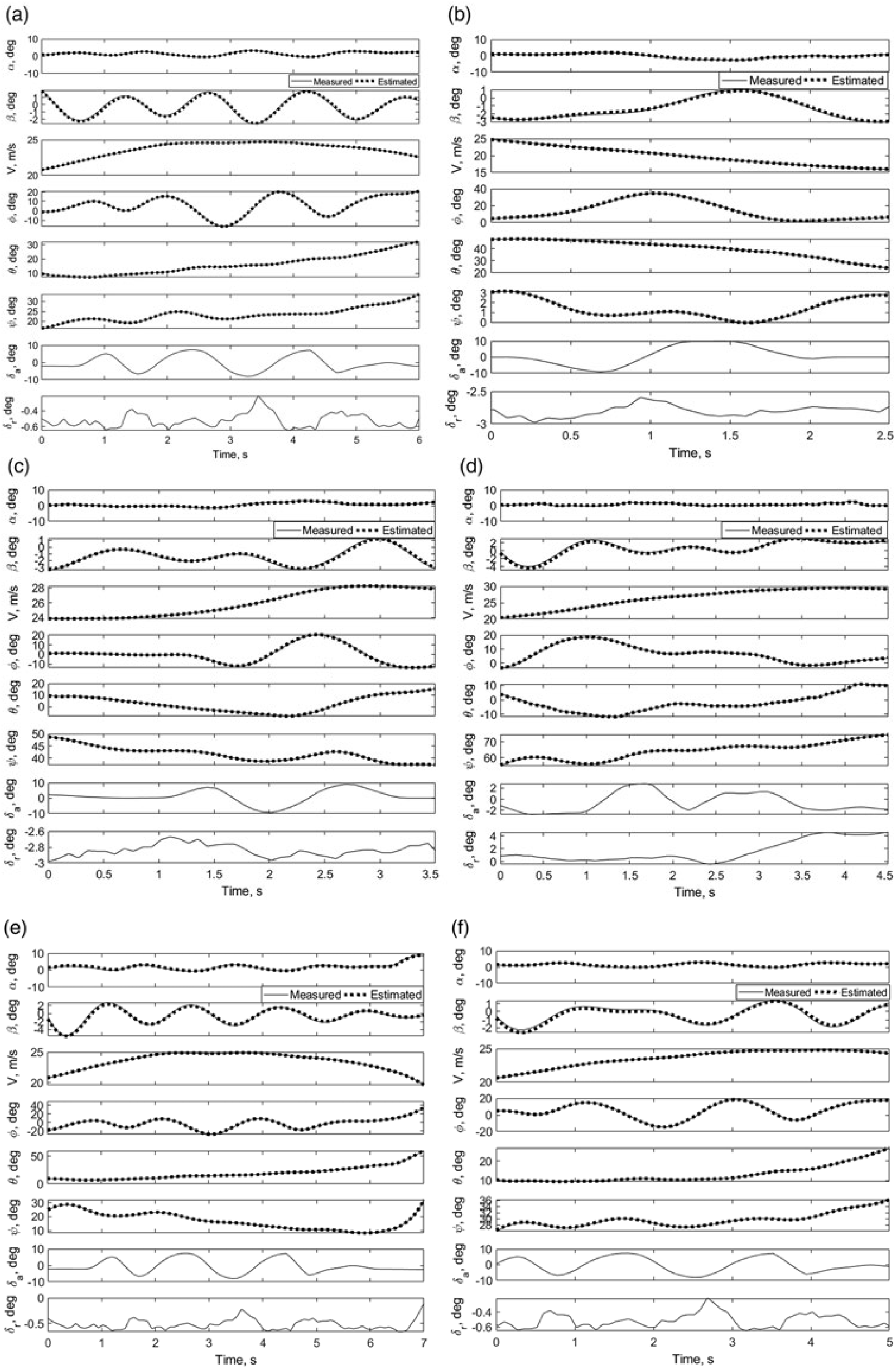
Figure 8. Data compatibility check of CDRW lateral-directional configuration: URW_LD1-LD6.
7.0 RESULTS AND DISCUSSION
Six flight data sets with nomenclature URW_LG1 to URW_LG6, generated with various elevator control inputs, are used to perform longitudinal aerodynamic characterisation using ML, LS and NGN methods. Similar methods are employed to carry out lateral-directional parameter estimation for six sets of flight data, namely URW_LD1 to URW_LD6, obtained from the manoeuvres with dominant aileron and rudder control inputs. While handling the estimation problem using the ML and NGN methods, which belong to a class of output error minimisation, the aim is to minimise the error between measured and simulated responses such as  $V_{\infty },\alpha ,\beta ,\emptyset ,\theta ,p,q,r,a_x,\ a_y,a_z$ with a set of guess parameters and the initial conditions as an input. In case of the LS method, parameters are estimated by minimising the error between measured and simulated dependent variables such as
  $C_L,C_D,C_Y,C_l,C_m$ and
  $C_n$. Since these aerodynamic coefficients cannot be measured directly during flight tests, instead they are reconstructed from measured independent variables using Equations (21)–(28). These reconstructed non-dimensional aerodynamic force and moment coefficients are treated as measured variables. Figures 9 and 10 present the estimated response of motion variables using the ML, NGN and LS methods for longitudinal and lateral-directional modes, respectively. For the ML and NGN methods, the response of motion variables is obtained as a part of the output, whereas in case of the LS method, the estimated parameters, which are the output, are used to simulate the respective dynamics using rigid body equations of motion presented in Equations (1)–(14).

Figure 9. Longitudinal parameter estimation of CDRW configuration.

Figure 10. Lateral-directional parameter estimation of CDRW configuration.
It can be observed from Figs. 7 and 9 that the variation in angle-of-attack for all the longitudinal manoeuvres is within the range of  ${\bf -10}^{\boldsymbol{\circ}} {\le \alpha \le} \textbf{10}^{\boldsymbol{\circ}}$. Referring to Fig. 4, which represents the variation of longitudinal aerodynamic force and moment coefficients with angle-of-attack from wind-tunnel testing, it can be noticed that the variation of
  ${\boldsymbol C}_{\boldsymbol L}$ is almost linear in the interval
  ${\boldsymbol -5}{{}^{\boldsymbol\circ}}\le {\boldsymbol\alpha}\le \textbf{10}{{}^{\boldsymbol\circ}}$ and the corresponding value of
  ${\boldsymbol C}_{{\boldsymbol L}_{\boldsymbol \alpha}}$ is 3.06. Although small but noticeable deviation from linearity in the variation of
  ${\boldsymbol C}_{\boldsymbol L}$ can be observed within the regime
  $\textbf{1}\textbf{0}{{}^{\boldsymbol\circ}}\le {\boldsymbol\alpha}\le \textbf{14}{{}^{\boldsymbol\circ}}$, beyond which there is a significant non-linearity followed by a stall at around
  ${\boldsymbol\alpha}\approx {\boldsymbol 21}^{\boldsymbol\circ}$. The
  ${\boldsymbol C}_{{\boldsymbol L}_{{\boldsymbol\alpha}}}$ in the angle-of-attack domain
  ${\boldsymbol -5}{{}^{\boldsymbol\circ}}\le {\boldsymbol\alpha}\le \textbf{14}{{}^{\boldsymbol\circ}}$ is 2.98, and its relative error w.r.t.
  ${\boldsymbol C}_{{\boldsymbol L}_{\boldsymbol\alpha}}$ in the regime
  ${\boldsymbol -5}{{}^{\boldsymbol\circ}}\le {\boldsymbol\alpha}\le \textbf{10}{{}^{\boldsymbol\circ}}$ is less than
  $3{\%}$. Hence, the variation in the aerodynamic coefficients is considered to be linear in the angle-of-attack regime
  ${\boldsymbol -5}{{}^{\boldsymbol\circ}}\le {\boldsymbol\alpha}\le \textbf{14}{{}^{\boldsymbol\circ}}$. As mentioned earlier, the variation in angle-of-attack for all the manoeuvres falls well within the considered linear regime, and hence, the postulated aerodynamic model in Equations (9)–(11) should be sufficient to capture the respective dynamics.
Figure 9(a)–(d) presents the estimation of longitudinal motion variables using the ML, LS and NGN methods. Referring Fig. 9, it is observed that the estimated motion variables are in close agreement with the corresponding measured data for the ML and NGN methods. It is also noticed that the maximum deviation in the estimated angle-of-attack, using the ML and NGN methods, is observed for the flight data URW_LG2 and URW_LG6, respectively. The corresponding deviation of  $\alpha $ w.r.t measured data is
  $\textbf{1}{{}^{\boldsymbol\circ}}$ and
  $\textbf{2}.\textbf{5}{{}^{\boldsymbol\circ}}$, respectively. Similarly, the maximum deviation in the pitch rate for the corresponding flight data sets is observed to be of the magnitude
  $\textbf{0}.\textbf{1} \text{rad/s}$ and 0.3 rad/s at a data point 1.1 s and 1.7 s, respectively. Referring Figs 8 and 10, it can be observed that the variation in the side slip during all the lateral-directional manoeuvres is in the range of
  ${\boldsymbol -5}{{}^{\boldsymbol\circ}}\le {\boldsymbol\beta}\le \textbf{6}{{}^{\boldsymbol\circ}}$, which is well within the linear regime according to the wind-tunnel results presented in Fig. 5. It is also observed from Fig. 10, barring data set URW_LD5, that the maximum deviation in the sideslip angle using the MLE and NGN methods is less than 1
 ${{}^{\boldsymbol\circ}}$ and
  $\textbf{0}.\textbf{5}{{}^{\boldsymbol\circ}},$ respectively. The corresponding deviation in the roll rates is
  $\textbf{0}.\textbf{05} \text{rad/s}$ and 0.025 rad/s, and the respective yaw rates the deviation is of the magnitude
  $\textbf{0}.\textbf{1} \text{rad/s}$ and 0.03 rad/s for the MLE and NGN methods, respectively. It is evident from the aforementioned discussion that the considered linear lateral-directional aerodynamic model is able to capture the lateral-directional dynamics.
From Figs. 9 and 10, it is observed that the trained neural model of NGN method is able to predict and match the measured flight data for majority of the flight data sets. This pattern following the ability of the trained neural network enables the NGN method to perform on par with the classical ML method. Major deviation of NGN estimates is observed from the figures related to the flight data sets URW_LG6 and URW_LD5. During the neural training for the NGN method, the control input is not considered as input for training but plays a vital role during the estimation process through the postulated aerodynamic model. Hence, the NGN method becomes sensitive to the kind of excitation and the respective training. On the other hand, the LS estimates show a significant deviation in the estimated response with the measured data. Interestingly, it is observed that the current URW configuration reaches the steady-state condition in a very short interval of time after the application of an excitation input.
The estimated longitudinal and lateral-directional parameters, along with Cramer-Rao bound and standard deviation from six sets of flight data, using the ML, LS and NGN methods, are presented in Table 4–7. Figures 11 and 12 present the corresponding scatter plots for the estimated derivatives, using aforementioned methods. Tables 8–9 quantify the mean and standard deviation of the estimates from six sets of longitudinal and six sets of lateral-directional flight data, respectively. It can be observed that the ML and NGN estimates of aerodynamic parameters are consistent and in close agreement with the wind-tunnel results of CDRW configuration(Reference Saderla29). The obtained lower values of Cramer-Rao bound enhance the confidence in the estimated parameters. There is a consistent and significant deviation in the estimated parameters using the LS method, which can be attributed to the fact that the LS method yields inconsistent and biased estimates in the presence of noise in the measured independent variables. Referring Tables 4–5, it can also be observed that the estimated values of pitch damping derivatives are very low in magnitude. For an aircraft with no dedicated horizontal tail, which is a major contributor for pitch damping, estimating  $C_{m_q}$ and
  $C_{L_q}$ is a challenging task. Though small in magnitude, consistent estimates of
  $C_{m_q}$ are observed from the scatter plots in Fig. 11, with the respective mean and standard deviation of −0.073 and 1.2% using the MLE method and −0.071 and 0.6% using the NGN method. It is also observed that the estimates of
  $C_{L_0}$ and
  $C_{m_0}$ are in a close match with the wind-tunnel values, and the respective relative error is less than 0.01%. A small but noticeable scatter is observed in the estimates of
  $C_{L_{\alpha }}$ and
  $C_{m_{\alpha ,}}$ but the percentage error of the mean w.r.t wind-tunnel values is close to 0.75% and 6.4% for the ML methods and 0.01% and 4.175% for the NGN methods. Due to the onboard acquisition of the approximate variation of thrust during maneuvers, the estimated profile drag parameter
  $C_{D_0}$ is close to the wind-tunnel measurements, with a relative error of mean from both the MLE and NGN methods close to 1%. It can be observed from Table 8 that the estimate of elevator control derivative
  $C_{m_{{\delta }_e}}$ is consistent, with a mean of −0.4037 and the respective standard deviation as low as 3.3%. Whereas the weak derivatives such as
  $C_{L_{{\delta }_e}}$ and
  $C_{L_q}$ are found to be fluctuating w.r.t wind-tunnel testing data. From Fig. 12, it is observed that the estimated lateral-directional bias parameters
  $C_{Y_0},\ C_{l_0}$ and
  $C_{n_0}$ deviate with a relative error of 0.01%. It is also noticed that the mean values of the estimated lateral-directional static stability derivatives,
  $C_{l_{\beta }}$ and
  $C_{n_{\beta }}$, are −0.089 and 0.021 using the MLE method and −0.055 and 0.015 using the NGN method. The corresponding deviation of these estimated derivatives from wind-tunnel measurements is 0.012 and 0.001 using the MLE method and 0.045 and 0.005 using the NGN method. It can be inferred from Fig. 12 that the estimates of roll and yaw damping derivatives,
  $C_{l_p}$ and
  $C_{n_r}$, using the MLE method, are consistent, with a mean of −0.5 and −0.067 and standard deviation of 0.7% and 1.9%, respectively. The offset estimates of
  $C_{l_p}$ and
  $C_{n_r}$ using the NGN method, are observed with URW_LD5 and URW_LD6, respectively. Barring respective data sets, the estimates of aforementioned derivatives are also consistent using the NGN method, with a corresponding mean of −0.48 and −0.031. The estimates of
  $C_{l_{{\delta }_a}}$ are also observed to be consistent using both the MLE and NGN methods, with a percentage deviation of mean w.r.t wind-tunnel estimate to be 0.8% and 0.6%, respectively, barring URW_LD5 NGN estimate. It is observed that the estimates, using both the MLE and NGN methods, of the derivatives
  $C_{Y_{{\delta }_r}},\ C_{l_{{\delta }_r}}$ and
  $C_{n_{{\delta }_r}}$ are inconsistent and have a significant deviation from wind-tunnel measurements. This may be attributed to the reason that the rudder control inputs during all the lateral-directional manoeuvres are almost negligible, which definitely limit the excitation of respective derivatives. As mentioned earlier, the CDRW configuration is equipped with a high-aspect-ratio all-movable vertical tail, because of which the UAV during flight tests is observed to be very sensitive for rudder inputs. Due to this reason, the pilot operating from ground station was not able to execute the designed rudder control inputs.
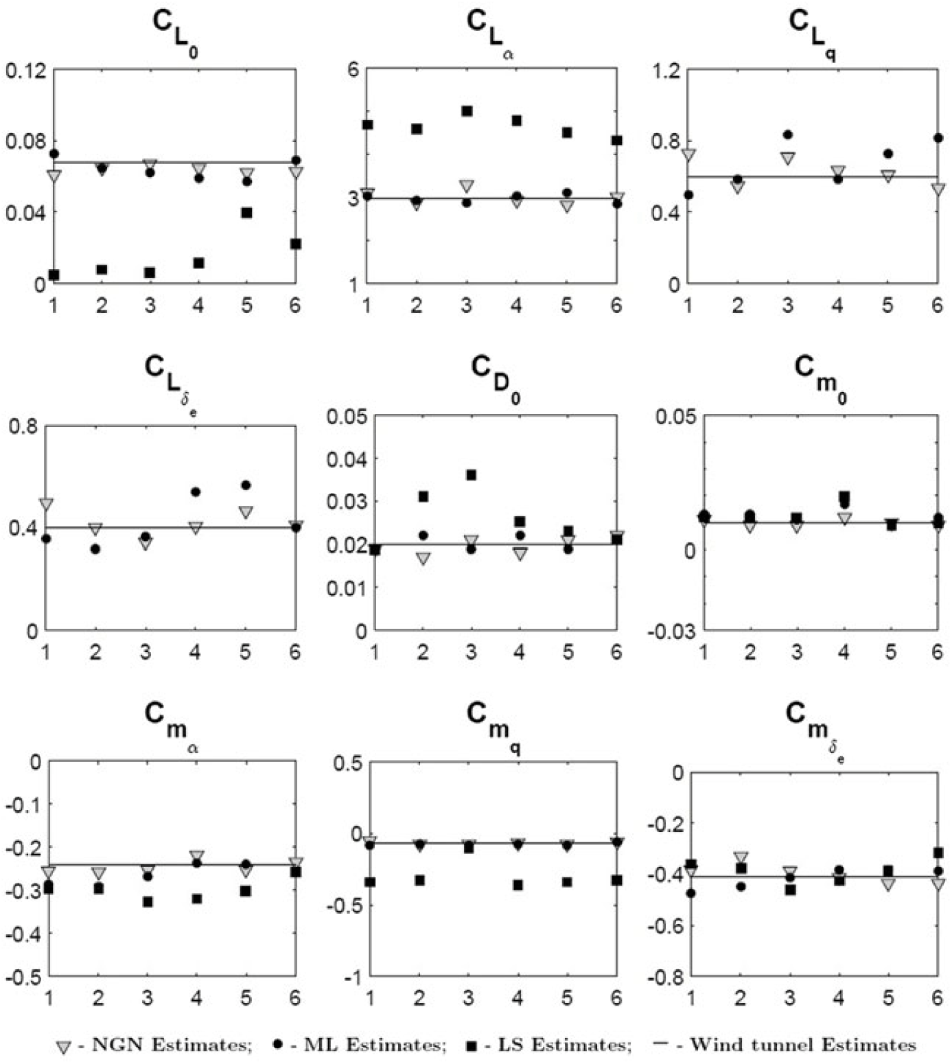
Figure 11. Scatter plot of parameter estimated using the ML, LS and NGN methods.

Figure 12. Scatter plot of lateral-directional parameters using the ML and LS methods for CDRW configuration.
Table 4 Estimated Longitudinal parameters of CDRW: URW_LG1, URW_LG2, and URW_LG3

Values in parentheses represent Cramer-Rao bound and those in square brackets, represent standard deviation.
Table 5 Estimated Longitudinal parameters of CDRW: URW_LG4, URW_LG5 and URW_LG6

Values in parentheses represent Cramer-Rao bound and those in square brackets represent standard deviation.
Table 6 Estimated parameters from lateral-directional flight data CDRW: URW_LD1, URW_LD2, and URW_LD3

Values in parentheses represent Cramer-Rao bound and those in with * represent standard deviation.
Table 7 Estimated Parameters from lateral-directional flight data CDRW: URW_LD4, URW_LD5, and URW_LD6

Values in parentheses represent Cramer-Rao bound and those in with * represent standard deviation.
Table 8 Mean of longitudinal estimates of CDRW using the ML, LS and NGN methods

Values in square brackets represent standard deviation.
Table 9 Mean of lateral-directional estimates of CDRW using the ML, LS and NGN methods

Values in square brackets represent standard deviation.
To validate the aerodynamic model and estimated parameters using the ML and NGN methods, proof-of-match exercise is performed for both longitudinal and lateral-directional motion, presented in Figs. 13 and 14, respectively. The validation task was performed by taking the mean of the estimated aerodynamic parameters obtained from the flight data URW_LG1, URW_LG2, URW_LG4 and URW_LG6, which are used to generate simulated outputs for elevator inputs of flight data URW_LG3 and URW_LG5, respectively. Similarly, simulated outputs are generated for elevator inputs of flight data URW_LD2 and URW_LD3 by using the mean of the aerodynamic parameters estimated from flight data URW_LD1, URW_LD4, URW_LD5 and URW_LD6. The aerodynamic model considered for estimation is kept constant during the exercise and six DOF equations of motion are used for computing the estimated response.

Figure 13. Proof-of-match exercise for longitudinal mode.

Figure 14. Proof-of-match exercise for lateral-directional mode.
8.0 CONCLUSION
Parameter estimation from flight tests of the designed CDRW configuration using the ML, LS and NGN methods over six sets of flight data pertaining to longitudinal and lateral/directional dynamics is performed. Estimated motion variables corresponding to longitudinal and lateral dynamics using the ML and NGN methods were able to match reasonably well with the measured flight data, with NGN requiring much more training to perform accurately for the lateral-directional case. Parameters estimated using the ML and NGN methods are consistent over six sets of flight data, and the corresponding mean is in close agreement with wind-tunnel estimates. The lower values of Cramer-Rao bounds establish a higher confidence level in the estimated parameters. The results from the ML and NGN methods were entrusted by the minimal scatter and a negligible standard deviation, whereas the estimates from the LS method displayed significant scatter and deviates from the ML and NGN methods and from wind-tunnel test results. The pattern following ability of the trained neural network enabled the NGN method to perform on par and better than the classical ML method upon extensive training of neural weights. The restriction in training of the neural network for a particular flight data set has been reflected during proof-of-match exercise. The quality of the estimates can be further improved by implementing the predecided input by a dedicated on-board controller. This task will maximise the possibility of exciting the manoeuvres with desired frequencies. The estimates from the ML and NGN methods were consistent and can be improved by a greater number of flight data sets for various flight regimes, which will enhance the confidence in generalising their application for parameter estimation of UAVs.


