NOMENCLATURE
 ${\alpha _1}$
The angle of rotation of the projectile around the
$x$ axis- ${\theta _1}$
The angle between the
$x$ axis and ${x_1}$ axis on the inner wing- ${\theta _2}$
The angle between the
$x$ axis and ${x_2}$ axis on the outer wing- ${\Phi _{\rm{q}}}$
Position constraint equation
- $\eta $
the acceleration tilt to the right
- $\rho $
air density
- ${\rm{f}}$
aerodynamic force
- $J$
Moment of inertia
- $K$
stiffness factor
- $t$
time
- $T$
kinetic energy
- $U$
Potential energy
- $v$
the speed tilt to the right
- $V$
air velocity
- $\omega $
oscillation frequency


1.0 INTRODUCTION
With the development of technology, more types of folding mechanisms are used in various fields. A folding wing is a type of missile wing connected to the body of the missile through a folding mechanism and can be folded in or on the surface of the body before the missile is launched. Folding wing technology has been used more frequently in recent years(Reference Ting and Lixin1). Folding wings have been widely used in projectile weapons because of their simple structure and small space requirement. During the storage, transportation, and launch of projectiles and arrows, the structural design of the projectile is usually changed to meet certain mechanical properties during the deployment process to reduce the lateral size of the projectile. The opening movement of the wing is a key factor to ensure that the projectile can achieve flight control. The spreading movement of the wing has two main forms: horizontal and vertical spreading. The former installs another wing surface in the axial direction at the root of the wing surface, enabling the outer wing portion to be folded and opened around the axis. The latter installs a rotation axis perpendicular to the surface near the root of the airfoil, enabling the wing to rotate around the axis. For some missiles, such as tactical and cruise missiles, box-type launching is used, that is, the wing is folded into the launch box before launching, and the wing is opened immediately after launch. Two methods for the missile folding wing deployment mechanism are currently used worldwide. The first one is divided into a gas-actuated cylinder type, an elastic drive type, and a motor-driven type according to the driving method, such as the folding type, the one-piece rotating type, the V-shaped rotating type, the cross-folding type, and flexible variant.
Many studies on the deployment of conventional wings have been conducted. For example, Dai(Reference Wenliu2) studied the entire process of the rudder wing mechanism of the guided projectile initiation to open and lock the wing and performed dynamic analysis on the movement process of the rudder wing opening. Zhen(Reference Zhen Wenqiang and Ji3) investigated the expansion of the folded wing during missile launch, established the mathematical model of aerodynamic drag and friction, and simulated the unfolding and locking process of the folding wing. Zhang(Reference Miaomiao4) conducted an innovative design and mechanics study of the unfolding mechanism of the folding wing surface. Ding(Reference Hong5) analysed and calculated the structural composition of a foldable tail of an aerial bomb and the deployment process of its components and studied the working stress level of the components and the dynamic behaviour of the deployment process. Wei studied the wing in the quasi-steady state (at a fixed angle) and in the deformed state, used the non-linear aeroelastic characteristics of Lagrangian equation to establish the structural model of the flap, and used the constraint equation to describe the deformation strategy of the flap. Keisuke Otsuka(Reference Otsuka, Wang and Makihara6) used a two-dimensional aerodynamic nonlinear flap model based on multi-body dynamics, absolute node coordinate formulas, and strip theory to simulate the unfolding motion of the aircraft in the time domain and studied the structural flexibility and aerodynamic instability impact on the time-domain deployment simulation. Within the scope of our knowledge, there are very few studies on the longitudinal secondary folding wing. Most of the studies are on the lateral secondary folding wing, and the lateral folding wing is widely used in aerospace and other fields, but for small and medium tactical missiles, the horizontal folding wing is not suitable for storage and launching, so it is necessary to study a longitudinal folding wing to meet the needs.
The dynamic process of folding wings opening is the research object of wings opening frequency from low to high. As the simulation steps are refined, the test factors to consider increase accordingly as well as the similarity of the test results. The low similarity model has a low computational cost and certain reference value for conceptual design, and it also paves the way for future practical design because the generation of real objects needs the support of conceptual design, which requires experimental simulation. The low-similarity model research developed a deployment system based on the conceptual design of the folding wing model. Given the limitations of the conditions, the system design was only implemented in the simulation environment, so the model ignored structural flexibility and aerodynamic instability, while the calculation amount was small. The accuracy of the test is lost, but the low-similarity model is necessary for data reference.
In this paper, a brand-new longitudinal secondary folding wing structure model is designed, and its aerodynamic characteristics in the unfolding process are studied. Firstly, the kinematic characteristics in the deformation process are analysed, and the dynamic equation is obtained; secondly, the generalised unsteady aerodynamic force is calculated, and the multi-body dynamic equation of the structure is obtained; then the flutter analysis of the folding wing is performed, and a vertical excitation is applied to a certain point of the folding wing to analyse its displacement response, acceleration response and angular freedom response during the unfolding process. Finally, the rationality of its structural design is verified by the combination of simulation experiment and physical experiment. The test data shows that the aeroelastic system of the folding wing will present different states. The aeroelastic response is not only sensitive to the initial conditions, but also sensitive to the folding angle.
2.0 STRUCTURE DYNAMICS MODELING
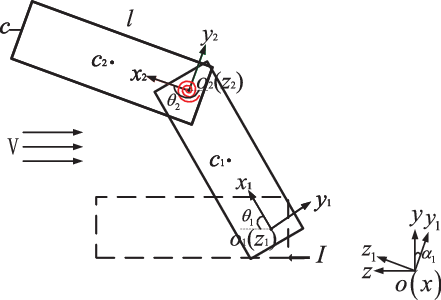
Figure 1 shows the schematic of the secondary longitudinal folding wing studied in this paper. In the theoretical modeling stage, the folding wing is simplified into two rigid parts(Reference Kwiatkowski7), namely, the inner and outer wings. Coordinate systems  ${O_1}{x_1}{y_1}{z_1}$ and
  ${O_2}{x_2}{y_2}{z_2}$ are attached to the inner and outer wing shafts, respectively, and the corresponding origins (
 ${O_1}$ and
  ${O_2}$) located at the centres of the two shafts can rotate universally. The
  $Oxyz$ coordinate system is a ground coordinate system located at the centre of the mass of the missiles. In the initial state, the apexes of the inner and outer wings are in contact with each other, that is, the inner and outer wings are folded into one.

Figure 1. Secondary longitudinal folding wing sketch.
Impulse is applied to the inner wing part so that it can rotate around the  ${z_1}$ axes, the inner wing drives the outer wing to rotate around the
  ${z_2}$ axis, and a rotating torsion spring is added along the
  ${z_2}$ axis. Under the action of external load, the folding wing makes a torsion movement around the x axis at the same time.
  ${\theta _1}$ is defined as the angle between the
  $x$ and
  ${x_1}$ axes on the inner wing;
  ${\alpha _1}$ is defined as the angle of rotation of the projectile about the
  ${x_1}$ axis;
  ${\theta _2}$ is defined as the angle between the
  $x$ and
  ${x_2}$ axes on the outer wing, around the
  ${z_1}$ axis the angle of rotation, so that the angle of the outer wing relative to the inner wing is
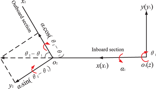
  ${\theta _2}{\rm{ - }}{\theta _1}$ as shown in the Fig. 2; and
  ${c_1}$ and
  ${c_2}$ are defined as the centroids of the inner and outer wing sections, respectively(Reference Hu, Yang, Gu and Wang8). The initial power source for the folding wing to expand is the gas produced by the combustion of the gunpowder acting on the piston, which causes the piston to advance and hit the edge of the inner wing. The mechanism model is simplified here, and the piston impact force is regarded as an impulse. If the inner and outer wings make rotational movements under the action of impulse and the Lagrange equation is used to establish the dynamic model of the folded wings, the specific process is as follows:

Figure 2. Diagram of rotating motion of the inner and outer wings.
2.1 Kinetic energy and potential energy of folding wing movement
The rotational inertia of the inner wing around the  ${z_1}$ axis is
 \begin{align}{J_{1{z_1}}} = \int_0^l {\int_{ - \frac{c}{2}}^{\frac{c}{2}} {\left( {{x^2} + {y^2}} \right)} } \frac{m}{{lc}}dxdy = \frac{m}{3}{l^2} + \frac{m}{{12}}{c^2}\end{align}
The rotational inertia of the inner wing around the  ${x_1}$ axis is
 \begin{align}{J_{1{x_1}}} = \frac{m}{{12}}{c^2}\end{align}
The rotational inertia of the outer wing around the  ${z_2}$ axis is
 \begin{align}{J_{2{z_2}}} = \int_0^l {\int_{ - \frac{c}{2}}^{\frac{c}{2}} {\left( {{x^2} + {y^2}} \right)} } \frac{m}{{lc}}dxdy = \frac{m}{3}{l^2} + \frac{m}{{12}}{c^2}\end{align}
The rotational inertia of the inner wing around the  ${x_2}$ axis is
 \begin{align}{J_{2{x_2}}} = \frac{m}{{12}}{c^2}\end{align}
The rotational inertia of the inner wing around the  ${y_2}$ axis is
 \begin{align}{J_{2{x_2}}} = \frac{m}{{12}}{l^2}\end{align}
The fin can be regarded as a rigid body rotating around an axis, as shown in Fig. 2. Thus, the kinetic energy of the system can be expressed as follows:
 \begin{align}{T_\theta } & = \frac{1}{2}{J_{1{z_1}}}\dot \theta _1^2 + \frac{1}{2}m\left( {\dot x_{{c_1}}^2 + \dot y_{{c_1}}^2} \right) + \frac{1}{2}{J_{2{z_2}}}{\left( {{{\dot \theta }_2} - {{\dot \theta }_1}} \right)^2} + \frac{1}{2}m\left( {\dot x_{{c_2}}^2 + \dot y_{{c_2}}^2} \right)\nonumber\\[5pt]{T_\alpha } & = \frac{1}{2}{J_{1x}}\dot \alpha _1^2 + \frac{1}{2}{J_{2{x_2}}}{\left[ {{{\dot \alpha }_1}\cos \left( {{\theta _2} - {\theta _1}} \right)} \right]^2} + \frac{1}{2}{J_{2{y_2}}}{\left[ {{{\dot \alpha }_1}\sin \left( {{\theta _2} - {\theta _1}} \right)} \right]^2}\end{align}
The equation above shows that the folding wing is two simplified rigid components, and the coordinates of the two centroids of the inner and outer wings are known. The coordinates are as follows:
 \begin{align}{x_{{c_1}}} & = \frac{1}{2}l\cos {\theta _1}\nonumber\\[4pt]{y_{{c_1}}} & = \frac{1}{2}l\sin {\theta _1}\nonumber\\[4pt]{x_{{c_2}}} & = l\cos {\theta _1} + \frac{1}{2}l\cos \left( {{\theta _2} - \pi } \right) = l\cos {\theta _1} - \frac{1}{2}l\cos {\theta _2}\nonumber\\[4pt]{y_{{c_2}}} & = l\sin {\theta _1} + \frac{1}{2}l\sin \left( {{\theta _2} - \pi } \right) = l\sin {\theta _1} - \frac{1}{2}l\sin {\theta _2}\end{align}
where  ${\dot x_{{c_1}}}$,
  ${\dot y_{{c_1}}}$,
  ${\dot x_{{c_2}}}$, and
  ${\dot y_{{c_1}}}$ can be obtained by differentiating the above equation:
 \begin{align}{\dot x_{{c_1}}} & = - \frac{1}{2}l{\dot \theta _1}\sin {\theta _1}\nonumber\\[4pt]{\dot y_{{c_1}}} & = \frac{1}{2}l{\dot \theta _1}\cos {\theta _1}\nonumber\\[4pt]{\dot x_{{c_2}}} & = - l{\dot \theta _1}\sin {\theta _1}{\rm{ + }}\frac{1}{2}l{\dot \theta _2}\sin {\theta _2}\nonumber\\[4pt]{\dot y_{{c_2}}} & = l{\dot \theta _1}\cos {\theta _1} - \frac{1}{2}l{\dot \theta _2}\cos {\theta _2}\end{align}
Thus,
 \begin{align}{\dot x^2}_{{c_2}} + {\dot y^2}_{{c_2}} = {l^2}\dot \theta _1^2 + \frac{1}{4}{l^2}\dot \theta _2^2 - {l^2}{\dot \theta _1}{\dot \theta _2}\cos \left( {{\theta _2} - {\theta _1}} \right)\end{align}
Substituting Eq. (9) into Eq. (6) yields
 \begin{align}{T_\theta } = \frac{1}{2}{J_{1{z_1}}}\dot \theta _1^2 + \frac{1}{8}m{l^2}\dot \theta _1^2 + \frac{1}{2}{J_{2{z_2}}}{\left( {{{\dot \theta }_2} - {{\dot \theta }_1}} \right)^2} + \frac{1}{2}m{l^2}\dot \theta _1^2 + \frac{1}{8}m{l^2}\dot \theta _2^2 - \frac{1}{2}m{l^2}{\dot \theta _1}{\dot \theta _2}\cos \left( {{\theta _2} - {\theta _1}} \right)\end{align}
By combining Eqs. (6) and (10), the kinetic energy equation of the system is obtained as follows(Reference Maiti, Roy, Mallik and Bhattacharjee9):
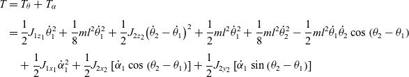 \begin{align}T & = {T_\theta } + {T_\alpha }\nonumber\\[4pt] & = \frac{1}{2}{J_{1{z_1}}}\dot \theta _1^2 + \frac{1}{8}m{l^2}\dot \theta _1^2 + \frac{1}{2}{J_{2{z_2}}}{\left( {{{\dot \theta }_2} - {{\dot \theta }_1}} \right)^2} + \frac{1}{2}m{l^2}\dot \theta _1^2 + \frac{1}{8}m{l^2}\dot \theta _2^2 - \frac{1}{2}m{l^2}{{\dot \theta }_1}{{\dot \theta }_2}\cos \left( {{\theta _2} - {\theta _1}} \right)\nonumber\\[4pt] &\quad + \frac{1}{2}{J_{1{x_1}}}\dot \alpha _1^2 + \frac{1}{2}{J_{2{x_2}}}\left[ {{{\dot \alpha }_1}\cos \left( {{\theta _2} - {\theta _1}} \right)} \right] + \frac{1}{2}{J_{2{y_2}}}\left[ {{{\dot \alpha }_1}\sin \left( {{\theta _2} - {\theta _1}} \right)} \right] \end{align}
The potential energy of the outer wing rotating motion caused by the torsion spring is
 \begin{align}U = \frac{1}{2}{K_2}{\left( {{\theta _2}{\rm{ - }}{\theta _1}} \right)^2}\end{align}
where the stiffness of  ${K_2}$ is assumed as
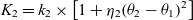 \begin{align}{K_2} = {k_2} \times \left[ {1 + {\eta _2}{{\left( {{\theta _2} - {\theta _1}} \right)}^2}} \right]\end{align}
2.2 Dynamic equation of opening motion
Let 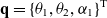 ${\textbf{q}} = {\left\{ {{\theta _1},{\theta _2},{\alpha _1}} \right\}^{\rm{T}}}$, then
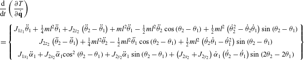 \begin{align} & \frac{\rm{d}}{{{\rm{d}}t}}\left( {\frac{{\partial T}}{{\partial {\dot{\textbf{q}}}}}} \right)\nonumber\\[5pt]& = \left\{ \begin{array}{c}{J_{1{z_1}}}{{\ddot \theta }_1} + \frac{1}{4}m{l^2}{{\ddot \theta }_1} + {J_{2{z_2}}}\left( {{{\ddot \theta }_2} - {{\ddot \theta }_1}} \right) + m{l^2}{{\ddot \theta }_1} - \frac{1}{2}m{l^2}{{\ddot \theta }_2}\cos \left( {{\theta _2} - {\theta _1}} \right) + \frac{1}{2}m{l^2}\left( {\dot \theta _2^2 - {{\dot \theta }_2}{{\dot \theta }_1}} \right)\sin \left( {{\theta _2} - {\theta _1}} \right)\\[5pt]{J_{2{z_2}}}\left( {{{\ddot \theta }_2} - {{\ddot \theta }_1}} \right) + \frac{1}{4}m{l^2}{{\ddot \theta }_2} - \frac{1}{2}m{l^2}{{\ddot \theta }_1}\cos \left( {{\theta _2} - {\theta _1}} \right) + \frac{1}{2}m{l^2}\left( {{{\dot \theta }_2}{{\dot \theta }_1} - \dot \theta _1^2} \right)\sin \left( {{\theta _2} - {\theta _1}} \right)\\[5pt]{J_{1{x_1}}}{{\ddot \alpha }_1} + {J_{2{x_2}}}{{\ddot \alpha }_1}{\cos ^2}\left( {{\theta _2} - {\theta _1}} \right) + {J_{2{y_2}}}{{\ddot \alpha }_1}\sin \left( {{\theta _2} - {\theta _1}} \right) + \left( {{J_{2{x_2}}} + {J_{2{y_2}}}} \right){{\dot \alpha }_1}\left( {{{\dot \theta }_2} - {{\dot \theta }_1}} \right)\sin \left( {2{\theta _2} - 2{\theta _1}} \right)\end{array} \right\}\nonumber\\[8pt]\end{align}
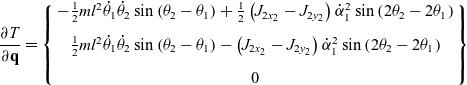 \begin{align}\frac{{\partial T}}{{\partial \textbf{q}}} = \left\{ \begin{array}{c} - \frac{1}{2}m{l^2}{{\dot \theta }_1}{{\dot \theta }_2}\sin \left( {{\theta _2} - {\theta _1}} \right) + \frac{1}{2}\left( {{J_{2{x_2}}} - {J_{2{y_2}}}} \right)\dot \alpha _1^2\sin \left( {2{\theta _2} - 2{\theta _1}} \right)\\[8pt]\frac{1}{2}m{l^2}{{\dot \theta }_1}{{\dot \theta }_2}\sin \left( {{\theta _2} - {\theta _1}} \right) - \left( {{J_{2{x_2}}} - {J_{2{y_2}}}} \right)\dot \alpha _1^2\sin \left( {2{\theta _2} - 2{\theta _1}} \right)\\[8pt]0\end{array} \right\}\end{align}
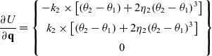 \begin{align}\frac{{\partial U}}{{\partial \textbf{q}}} = \left\{ \begin{array}{c} - {k_2} \times \left[ {\left( {{\theta _2} - {\theta _1}} \right) + 2{\eta _2}{{\left( {{\theta _2} - {\theta _1}} \right)}^3}} \right]\\[5pt]{k_2} \times \left[ {\left( {{\theta _2} - {\theta _1}} \right) + 2{\eta _2}{{\left( {{\theta _2} - {\theta _1}} \right)}^3}} \right]\\[5pt]0\end{array} \right\}\end{align}
The change function of the folding angle can be defined as  $\Delta \theta \left( t \right)$, and then the deformation equation of the folding angle is established as follows:
 \begin{align}\theta \left( t \right) = {\theta _2}\left( t \right) - {\theta _1}\left( t \right) = {\theta _2}\left( 0 \right) - {\theta _1}\left( 0 \right) + \Delta \theta \left( t \right)\end{align}
Considering the kinematics analysis, driving constraints must be imposed on the system to have a definite motion if the actual degree of freedom of the system is zero. Given that the analysis of the rotating motion of the folding wing is the position, speed, acceleration, and restraint reaction force of the system, the restraint equation of the system is expressed as
 \begin{align}{\Phi _q}\left( {\textbf{q},t} \right) = \left\{ {\left[ {{\theta _2}\left( t \right) - {\theta _1}\left( t \right)} \right] - \left[ {{\theta _2}\left( 0 \right) - {\theta _1}\left( 0 \right)} \right] - \Delta \theta \left( t \right)} \right\} = 0\end{align}
Eq. (18) of the Lagrangian multiplier theorem is used for processing. Assume  $q \in {R^n}$
 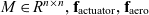 $M \in {R^{n \times n}}, \textbf{f}_{\mathrm{actuator}},\textbf{f}_{\mathrm{aero}}$
  ${\Phi _{\rm{q}}} \in {R^{m \times n}}$, then there is the Lagrange Multiplier Vector
  $\lambda \in {R^m}$.
By combining Eqs. (14), (16), and (18), we can obtain the dynamic equation of the folding wings during the opening movement:
 \begin{align}\begin{array}{l}\textbf{M}\left( {\textbf{q},t} \right)\ddot{\textbf{q}} + \textbf{K}\left( {\textbf{q},t} \right) + \Phi _q^T\left( {\textbf{q},t} \right)\lambda = {\textbf{f}_{{\rm{actuator}}}} + {\textbf{f}_{{\rm{aero}}}}\\[5pt]\Phi \left( {\textbf{q},t} \right) = 0\end{array}\end{align}
where  $\textbf{M}$ and
  ${\textbf{K}}$ are the mass and stiffness matrices, respectively, which are functions of
  ${\rm{q}}$; Λ is the Lagrange multiplier;
  ${\textbf{f}_{{\rm{actuator}}}}$ is generated by the movement of the outer wing and a function of
  ${\textbf{q}}$ and
  $\dot{\textbf{q}}$; and
  ${\Phi _q}$ is the constrained Jacobian matrix. The matrix is the position constraint equation.
 \begin{align}\textbf{M} & = \left[ {\begin{array}{ccc}{{J_{1{z_1}}} + \frac{5}{4}m{l^2}} & { - \frac{1}{2}m{l^2}\cos \left( {{\theta _2} - {\theta _1}} \right)} & 0\\[5pt]{ - {J_{2{z_2}}} - \frac{1}{2}m{l^2}\cos \left( {{\theta _2} - {\theta _1}} \right)} & {{J_{2{z_2}}} + \frac{1}{4}m{l^2}} & 0\\[5pt]0 & 0 & {{J_{1{x_1}}} + {J_{2{x_2}}}{{\cos }^2}\left( {{\theta _2} - {\theta _1}} \right) + {J_{2{y_2}}}\sin \left( {{\theta _2} - {\theta _1}} \right)}\end{array}} \right]\nonumber\\[12pt]\textbf{K} & = \left[ {\begin{array}{ccc}{{k_2} \times \left[ {1 + {\eta _2}{{\left( {{\theta _2} - {\theta _1}} \right)}^2}} \right]} & o & o\\[5pt]0 & {{k_2} \times \left[ {1 + {\eta _2}{{\left( {{\theta _2} - {\theta _1}} \right)}^2}} \right]} & 0\\[5pt]0 & 0 & 0\end{array}} \right]\nonumber\\[8pt]{\Phi _q} & = \left\{ { - 1,1,0} \right\}\nonumber\\[8pt]{\textbf{f}_{{\rm{actuator}}}} & = \left\{ {\begin{array}{ccc}{ - \frac{1}{2}m{l^2}{{\dot \theta }_2}{{\dot \theta }_1}\sin \left( {{\theta _2} - {\theta _1}} \right) + \frac{1}{2}\left( {{J_{2{x_2}}} - {J_{2{y_2}}}} \right)\dot \alpha _1^2\sin \left( {2{\theta _2} - 2{\theta _1}} \right) - \frac{1}{2}m{l^2}\left( {\dot \theta _2^2 - {{\dot \theta }_2}{{\dot \theta }_1}} \right)\sin \left( {{\theta _2} - {\theta _1}} \right)}\\[5pt]{ - \frac{1}{2}m{l^2}\dot \theta _1^2\sin \left( {{\theta _2} - {\theta _1}} \right) - \frac{1}{2}\left( {{J_{2{x_2}}} - {J_{2{y_2}}}} \right)\dot \alpha _1^2\sin \left( {2{\theta _2} - 2{\theta _1}} \right)}\\[5pt]{ - \left( {{J_{2{x_2}}} + {J_{2{y_2}}}} \right){{\dot \alpha }_1}\left( {{{\dot \theta }_2} - {{\dot \theta }_1}} \right)\sin \left( {2{\theta _2} - 2{\theta _1}} \right)}\end{array}} \right\}\end{align}
 ${\textbf{f}_{{\rm{aero}}}}$ is the aerodynamic vector, which is provided in the next section. Eq. (19) obtains the first and second derivatives of time to obtain the constraint equations for speed and acceleration.
 \begin{align}\dot \Phi \left( {\textbf{q}, \dot{\textbf{q}},t} \right) & = {\Phi _{\textbf{q}}}\left( {\textbf{q},t} \right)\dot{\textbf{q}} - v\left( {\textbf{q},t} \right) = 0\nonumber\\[5pt]\ddot\Phi \left( {\textbf{q},\dot{\textbf{q}},\ddot{\textbf{q}},t} \right) & = {\Phi _{\textbf{q}}}\left( {\textbf{q},t} \right)\ddot{\textbf{q}} - \eta \left( {\textbf{q}{\rm{,}}\dot{\textbf{q}},t} \right) = 0\end{align}
where  $v = - {\Phi _t}\left( {\textbf{q},t} \right)$ is called the speed tilt to the right, and
 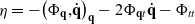 $\eta = - {\left( {{\Phi _{\textbf{q}}}{\rm{,}}\dot{\textbf{q}}} \right)_{\textbf{q}}} - 2{\Phi _{\textbf{q}t}}\dot{\textbf{q}} - {\Phi _{tt}}$ is called the acceleration tilt to the right. Given the initial conditions of the equation,
 \begin{align}\left.\begin{array}{l}\textbf{q}\left( 0 \right) = {\textbf{q}_0}\\[5pt]\dot{\textbf{q}}\left(0\right) = {{\dot{\textbf{q}}}_0}\end{array} \right\}\end{align}
3.0 AERODYNAMICS MODEL
3.1 Unsteady aerodynamic model
During the opening movement of the folding wing mechanism, the wing will change with the movement of the air, causing the system to generate additional unsteady aerodynamic forces, which affect the stability of the structure(Reference Zhao and Hu10). The geometric position and geometry of the inner and outer wings will also exhibit relative change. The influence of aerodynamic force will become very small when the deformation rate is small. To study the aeroelastic response of the folding wings during the expansion process, the aerodynamic model must be effectively reconstructed. In this study, the dipole grid method is used to calculate the generalised unsteady aerodynamic force(Reference Hu, Yang and Gu11). The wing surface is divided into grids, the lifting surface is discretised, and the area fraction is converted into a line integral. The following linear equation can be obtained, that is, the entire wing surface downwashing speed of the i th grid control point:
 \begin{align}{W_i} = \sum\nolimits_j {\frac{1}{{8\pi }}} \Delta {c_{pj}}\Delta {x_j}\cos {X_j}\int_{lj} {{k_{ij}}dl} \end{align}
In the formula, k is the kernel function, subscript i indicates the i
th
grid, subscript j indicates the j
th
grid,  $\Delta {c_{pj}}$ is the difference between the pressure coefficients on the j
th
grid, and
$\Delta {c_{pj}}$ is the difference between the pressure coefficients on the j
th
grid, and  $\Delta {x_j}$ is the j
th
grid. The average chord length of the lattice,
$\Delta {x_j}$ is the j
th
grid. The average chord length of the lattice,  ${X_j}$ is the sweep angle of the j
th
grid dipole line, and
${X_j}$ is the sweep angle of the j
th
grid dipole line, and  ${l_i}$ is the length of the i
th
grid dipole line.
${l_i}$ is the length of the i
th
grid dipole line.
All control points are expressed in matrix form as follows:
 \begin{align}\left\{ W \right\} = \left[ D \right]\left\{ {\Delta {c_p}} \right\}\end{align}
In the formula,  $\left[ D \right]$ is the aerodynamic influence coefficient matrix, that is,
 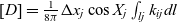 $\left[ D \right] = \frac{1}{{8\pi }}\Delta {x_j}\cos {X_j}\int_{lj} {{k_{ij}}dl} $.
The physical conditions at this time are expressed as
 \begin{align}W = \left( {i\frac{k}{b}f + \frac{{\partial f}}{{\partial x}}} \right)\end{align}
where b is the reference length, and f is the vibration mode corresponding to the aerodynamic model, which can be obtained from the principle of modal superposition:
 \begin{align}f = \left[ {{\Phi _H}} \right]\left\{ y \right\}\end{align}
In the formula,  $\left[ {{\Phi _H}} \right]$ is the vibration mode corresponding to each control point on the pneumatic panel, which can be obtained by surface spline interpolation; and
  $\left\{ y \right\}$ is the generalised coordinate.
According to Eq. (23) to Eq. (26), pressure coefficient difference  $\Delta {c_p}$ is expressed as
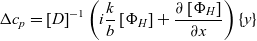 \begin{align}\Delta {c_p} = {\left[ D \right]^{ - 1}}\left( {i\frac{k}{b}\left[ {{\Phi _H}} \right] + \frac{{\partial \left[ {{\Phi _H}} \right]}}{{\partial x}}} \right)\left\{ y \right\}\end{align}
Both ends are divided by the generalised displacement vector  $\left\{ y \right\}$ to obtain the expression of dimensionless pressure coefficient difference
  $\overline {\Delta {c_p}} $ :
 \begin{align}\overline {\Delta {c_p}} = {\left[ D \right]^{ - 1}}\left( {i\frac{k}{b}\left[ {{\Phi _H}} \right] + \frac{{\partial \left[ {{\Phi _H}} \right]}}{{\partial x}}} \right)\end{align}
According to the relationship between the pressure and the pressure coefficient difference and the pressure coefficient difference expressed as Eq. (27), the generalised unsteady aerodynamic force can be obtained as
 \begin{align}\textbf{f} = \frac{1}{2}\rho {V^2}AIC\left( k \right)y\end{align}
In the formula,  $AIC\left( k \right)$ is the matrix of the unsteady aerodynamic influence coefficient and expressed as follows:
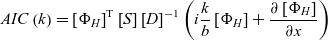 \begin{align}AIC\left( k \right) = {\left[ {{\Phi _H}} \right]^{\rm{T}}}\left[ S \right]{\left[ D \right]^{ - 1}}\left( {i\frac{k}{b}\left[ {{\Phi _H}} \right] + \frac{{\partial \left[ {{\Phi _H}} \right]}}{{\partial x}}} \right)\end{align}
The aerodynamic mesh is divided on the inner and outer wing surfaces, and the aerodynamic mesh and structural nodes do not overlap; therefore, it is necessary to use spline interpolation technology(Reference Harder and Desmarais12) to realise the interpolation relationship between the displacement of the aerodynamic mesh node and the structural mesh node displacement. After obtaining the unsteady aerodynamic influence coefficient matrix, derive it in the frequency domain and then obtain the aerodynamic force at the structural grid point. Using the dipole grid method(Reference Zhao and Hu13), a fixed angle is selected, and unsteady aerodynamic influence coefficient matrix  $AIC\left( k \right)$ is represented by
  $A\left( \omega \right)$. Then, it can be derived in the frequency domain, and then the folding wing displacement. The aerodynamics of the folding wings are linked as(Reference Duchon14)
 \begin{align}\textbf{f} = \frac{1}{2}\rho {V^2}A\left( \omega \right)y\end{align}
where ρ is the air density, V is the air velocity, and  $\omega$ is the oscillation frequency, which is used to indicate that the unsteady aerodynamic influence coefficient matrix is in the frequency domain. f and y are the gas and displacement vectors of the folded wings, respectively.
If the inner and outer wings are rectangular rigid bodies, the aerodynamic model can be interpolated to the four vertices of each section according to the spline interpolation technique. Spline matrix  ${{\rm{G}}_s}$ is a transformation from structural grid point
  ${y_s}$ to aerodynamic grid point displacement
  $y$, and the spline interpolation technique connects the four vertex deflectors of the inner and outer wing sections with the deflectors of the aerodynamic grid points through spline matrix
  ${{\rm{G}}_s}$, that is,
 \begin{align}y = {{\rm{G}}_s}{y_s}\end{align}
According to the principle of virtual displacement, the aerodynamic force ( $\textbf{f}$) and equivalent value (
 ${f_s}$) acting on the structural grid points should be equal to the work done at a certain virtual displacement to obtain
 \begin{align}\delta {y^{\rm{T}}}\textbf{f} = \delta y_s^{\rm{T}}{\textbf{f}_s}\end{align}
where  ${\textbf{f}_s}$ is the force vector of the interpolated structural node perpendicular to the surface.
Eq. (32) is introduced into Eq. (33) to obtain Eq. (34):
 \begin{align}\delta y_s^{\rm{T}}\left( {{\rm{G}}_s^{\rm{T}}f - {f_s}} \right) = 0\end{align}
Thus,
 \begin{align}{\textbf{f}_s} = {\rm{G}}_s^{\rm{T}}\textbf{f}\end{align}
Eqs. (32) and (35) are introduced into Eq. (31) to obtain a simplified aerodynamic model:
 \begin{align}{\textbf{f}_s} = \frac{1}{2}\rho {V^2}{A_{ss}}\left( \omega \right){y_s}\end{align}
where 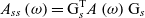 ${A_{ss}}\left( \omega \right){\rm{ = G}}_s^{\rm{T}}A\left( \omega \right){{\rm{G}}_s}$.
In this study, genetic algorithms can be used to optimise the position of the interpolated structural nodes. When performing aeroelastic analysis, it is necessary to provide a way of interconnection between structure and aerodynamic force. In order to connect the aerodynamic grid with the structural grid, the displacement at the structural grid point needs to be transformed into the displacement at the aerodynamic grid point. Design variable P is the identification number of the structural node, which is used to describe the position of each structural node. The optimisation problem is mathematically defined as follows(Reference Xuewen, Guifeng and Qingna15):
 \[\begin{gathered}
\begin{array}{*{20}{c}}
{{\text{Minimize}}:\sum\nolimits_{\theta = {\theta _0}}^{{\theta _n}} {{{\left( {\left| {\frac{{\overline {{V_f}} - {V_f}}}{{{V_f}}}} \right| + \left| {\frac{{\overline {{\omega _f}} - {\omega _f}}}{{{\omega _f}}}} \right|} \right)}_\theta }} } \\
\end{array} \\
{\text{Subject}}\;{\text{to }}\left\{ {\begin{array}{*{20}{c}}
{node\_I{D_{\min }}{\text{ }} < {P_i}{\text{ }} < node\_I{D_{\max }}} \\
{{P_i} \ne {P_j}} \\
\end{array} } \right.\left( {1 \le i \ne j \le {N_s}} \right) \\
\end{gathered} \]
\[\begin{gathered}
\begin{array}{*{20}{c}}
{{\text{Minimize}}:\sum\nolimits_{\theta = {\theta _0}}^{{\theta _n}} {{{\left( {\left| {\frac{{\overline {{V_f}} - {V_f}}}{{{V_f}}}} \right| + \left| {\frac{{\overline {{\omega _f}} - {\omega _f}}}{{{\omega _f}}}} \right|} \right)}_\theta }} } \\
\end{array} \\
{\text{Subject}}\;{\text{to }}\left\{ {\begin{array}{*{20}{c}}
{node\_I{D_{\min }}{\text{ }} < {P_i}{\text{ }} < node\_I{D_{\max }}} \\
{{P_i} \ne {P_j}} \\
\end{array} } \right.\left( {1 \le i \ne j \le {N_s}} \right) \\
\end{gathered} \]
 $\theta $ is the rotation angle,
  ${V_f}$ and
  $\overline {{V_f}} $ are the respective flutter speeds before and after simplification, and
  ${\omega _f}$ and
  $\overline {{\omega _f}} $ are the flutter frequencies before and after simplification, respectively. Using the common denominator root can more effectively approximate the aerodynamic impact coefficient.
 \begin{align}\left[ {{A_{ap}}} \right] = \left[ {{P_0}} \right] + \left[ {{P_1}} \right]\overline s + \left[ {{P_2}} \right]{\overline s ^2} + \sum\nolimits_{j = 3}^N {\frac{{\left[ {{P_j}} \right]{{\overline s }^j}}}{{j + {\gamma _{j - 2}}}}} \end{align}
The value of  ${\gamma _{j - 2}}$ is selected within the reduced frequency range of interest. Real coefficient matrix
  $\left[ P \right]$ is obtained by setting
  $\overline s = ik$ and fitting the table-column oscillation coefficient matrix item by item using the least squares(Reference Snyder, Sanders, Eastep and Frank16). Then,
 \begin{align}\left[ {{A_{ap}}} \right] = {\left( {\overline s \left[ I \right] - \left[ R \right]} \right)^{ - 1}}\left( {\left[ {{P_1}} \right]{{\overline s }^2} + \left[ {{P_2}} \right]\overline s + \left[ {{P_3}} \right]} \right)\end{align}
After obtaining the simplified aerodynamic model in the frequency domain, the aerodynamic model is transformed into the time domain using the minimum state (Eqs. (37), (38), (39)), and the unsteady aerodynamic model can be expressed as
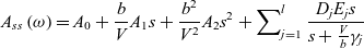 \begin{align}{A_{ss}}\left( \omega \right) = {A_0} + \frac{b}{V}{A_1}s + \frac{{{b^2}}}{{{V^2}}}{A_2}{s^2} + \sum\nolimits_{j = 1}^l {\frac{{{D_j}{E_j}s}}{{s + \frac{V}{b}{\gamma _j}}}} \end{align}
where  ${D_j}$ is a matrix;
  ${E_j}$ is a row matrix;
  $s$ is a pull-type complex variable; and
  ${A_0}$,
  ${A_1}$,
  ${A_2}$, and
  ${D_j}$,
  ${E_j}$ are the matrices to be obtained. The aerodynamic model of Eq. (36) can be transformed into a time-domain aerodynamic model by approximating the rational function.
 \begin{align}{\textbf{f}_s} = \frac{1}{2}\rho {V^2}\left[ {{A_0} + \frac{b}{V}{A_1}s + \frac{{{b^2}}}{{{V^2}}}{A_2}{s^2}} \right]{y_s} + \frac{1}{2}\rho {V^2}D{\left[ {sI - \frac{V}{b}R} \right]^{ - 1}}Es{y_s}\end{align}
As shown in Eq. (41), the aerodynamic model of the folded wing at a fixed rotation angle can be expressed by a coefficient matrix.
3.2 Aeroelastic system modeling
If the structural model is connected with the aerodynamic model, then the relationship between  ${\textbf{f}_{aero}}$,
  ${\textbf{f}_s}$,
  ${y_s}$, and
  $\textbf{q}$ must be established. The aeroelastic problem involves the interaction between aerodynamics and the structure. Spline technology is used to connect the structural and aerodynamic models. The steady aerodynamic force is coupled with the structural model, bringing Eq. (41) into Eq. (20)(Reference Selitrennik and Karpel17). The aerodynamic model simplifies the airfoil surface into a lifting surface. Based on its own dynamics and kinematics equations, this article describes the relationship between the motion parameters and the projectile body and flight control variables, while the structural model is a simplified rigid body that simulates the stiffness and weight distribution.
Assuming that torsion angle  ${\alpha _1}$ and rotation angle
  ${\theta _1}$,
  ${\theta _2}$ are very small during the opening of the folding wing, relative folding angle
  ${\theta _2}{\rm{ - }}{\theta _1}$ is also very small. Thus,
  $\sin {\theta _1} \approx {\theta _1}$,
  $\sin {\alpha _1} \approx {\alpha _1}$, and
  $\tan {\alpha _1} \approx {\alpha _1}$. The displacement coordinate of the i
th
vertex of the normal surface of the inner wing can be expressed as
$\tan {\alpha _1} \approx {\alpha _1}$. The displacement coordinate of the i
th
vertex of the normal surface of the inner wing can be expressed as
 \begin{align}{y_{s1i}} = {x_{1i}}{\theta _1} - {z_{1i}}{\alpha _1}\left( {i = 1,2,3,4} \right)\end{align}
In the formula,  $i$ denotes the different inner side coordinate points, and
  ${x_{1i}}$ and
  ${z_{1i}}$ are the coordinate values of the i
th
coordinate point in the local coordinate system.
${z_{1i}}$ are the coordinate values of the i
th
coordinate point in the local coordinate system.
The displacement coordinates of the  ${j^{th}}$ vertex of the outer wing normal surface can be expressed as
 \begin{align}{y_{s2j}} = l{\theta _1} - {x_{2j}}\cos {\theta _2} - {z_{2j}}{\alpha _1}\left( {j = 1,2,3,4} \right)\end{align}
where  $l{\theta _1}$ is the displacement value change caused by the rotation of a node on the inner wing surface around the
  ${z_1}$ axis,
  ${x_{2j}}\cos {\theta _2}$ is the displacement value change caused by the rotation of a node on the outer wing surface around the
  ${z_2}$ axis, and
  ${z_{2i}}{\alpha _1}$ is the displacement value change caused by the torsional movement of a node on the outer wing surface around the
  ${x_1}$ axis.
  ${x_{2j}}$ and
  ${z_{2j}}$ are the coordinate values of the
  ${j^{th}}$ vertex in local coordinate system
  ${x_2}{y_2}{z_2}$.
Therefore, the relationships between q and  ${y_s}$ and between
  ${\textbf{f}_{aero}}$ and
  ${\textbf{f}_s}$ can be obtained by introducing Eqs. (42) and (43) into Eq. (41):
 \begin{align} {\textbf{f}_{aero}} & = {{\rm{S}}^{\rm{T}}}{\textbf{f}_s}\nonumber\\[5pt]& = \frac{1}{2}\rho {V^2}{{\rm{S}}^{\rm{T}}}{A_0}{y_s}{\rm{ + }}\frac{1}{2}b\rho V{{\rm{S}}^{\rm{T}}}{A_1}{{\dot y}_s} + \frac{1}{2}{b^2}\rho {{\rm{S}}^{\rm{T}}}{A_2}{{\ddot y}_s}\nonumber\\[5pt]& + \frac{1}{2}\rho {V^2}{{\rm{S}}^{\rm{T}}}D{\left[ {sI - \frac{V}{b}\hat R} \right]^{ - 1}}E{{\dot y}_s}\end{align}
Let
 \begin{align}{x_a} = {\left[ {sI - \frac{V}{b}\hat R} \right]^{ - 1}}E\left( {{\rm{S\dot{\rm q}}} + {{\rm{S}}_{FA}}{{\dot \alpha }_{FA}}} \right)\end{align}
Bringing Eq. (44) and Eq. (45) into Eq. (20), the aeroelastic equation of folding wings is obtained as follow(Reference Attar, Tang and Dowell18):
 \begin{align}{\rm{M}}\left( {\textbf{q},t} \right)\ddot{\textbf{q}} + {\rm{K}}\left( {\textbf{q},t} \right)\textbf{q} + \Phi _{\textbf{q}}^T\left( {\textbf{q},t} \right)\lambda =\, & {\textbf{f}_{actuator}} + {\tilde A_0}\textbf{q} + {\tilde A_1}\dot{\textbf{q}} + {\tilde A_1}{\dot \alpha _{FA}} + {\tilde A_2}{{\ddot{\textbf{q}} + }}{\mathord{\buildrel{\lower3pt\hbox{$\scriptscriptstyle\smile$}} \over A} _2}{\ddot \alpha _{FA}}\nonumber\\[5pt]& + \tilde D{x_a} \Phi \left( {\textbf{q},t} \right) = 0\end{align}
To solve the algebraic differential equation of Eq. (46), Eq. (46) is transformed into multibody dynamic Eq. (47)(Reference Fujita and Nagai19):
 \begin{align}\left[ \begin{array}{cc}\textbf{M} & {\Phi _{\textbf{q}}^{\rm{T}}}\\[5pt]{\Phi _{\textbf{q}}} & 0\end{array} \right]\left\{ \begin{array}{c}\ddot{\textbf{q}}\\[5pt]\lambda \end{array} \right\} = \left\{ \begin{array}{c} - \textbf{Kq} + {\textbf{f}_{actuator}} + {{\tilde A}_0}\textbf{q} + {{\tilde A}_1}\dot{\textbf{q}} + {{\tilde A}_1}{{\dot \alpha }_{FA}} + {{\tilde A}_2}\ddot{\textbf{q}} + {\mathord{\buildrel{\lower3pt\hbox{$\scriptscriptstyle\smile$}} \over A} _2} {{\ddot \alpha }_{FA}} + \tilde D{x_a}\\[5pt]\gamma \end{array} \right\}\end{align}
According to constrained Jacobian matrix Eq. (18),
 \begin{align}\Phi_{\textbf{q}}\dot{\textbf{q}} = - {\Phi_t}\end{align}
where  $\Phi_{\textbf{q}}$ and
  ${\Phi _t}$ are the partial derivatives of
  $\Phi $ with respect to
  $\textbf{q}$ and
  $t$, respectively.
By deriving t for Eq. (48), we can obtain Eq. (49):
 \begin{align}{\Phi _{\textbf{q}}}\ddot{\textbf{q}} = - {\Phi _{tt}} - 2{\Phi _{\textbf{q}t}}{\Phi _{tt}} - {\left( {{\Phi _{\textbf{q}}}\dot{\textbf{q}}} \right)_{\textbf{q}}}\dot{\textbf{q}}\end{align}
where  ${\Phi _{tt}}$ is the second-order partial derivative of
  $\Phi $ on
  $t$,
$t$,  ${\Phi _{\textbf{q}t}}$ is the partial derivative of
  $\Phi $ on
  $\textbf{q}$ and
  $t$, and
  $\left( {{\Phi _{\textbf{q}}}\dot{\textbf{q}}} \right)_{\textbf{q}}$ is the partial derivative of
  ${\Phi _{\textbf{q}}}\dot{\textbf{q}}$ on
  $\textbf{q}$. Let
 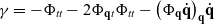 $\gamma = - {\Phi _{tt}} - 2{\Phi _{\textbf{q}t}}{\Phi _{tt}} - {\left( {{\Phi _{\textbf{q}}}\dot{\textbf{q}}} \right)_{\textbf{q}}}\dot{\textbf{q}}$, then
  ${\rm{M}}$ and
  ${\rm{K}}$ are mass and stiffness matrices, which are functions of
  $\textbf{q}$.
Multiply the left side of Eq. (45) by  $\left( {sI - \frac{V}{b}\dot R} \right)$, and after conversion, we get
 \begin{align}{\dot x_a} = \frac{V}{b}\hat R{x_a} + \hat ES{\dot{\rm q}} + \hat E{S_{{\rm{FA}}}}{\dot \alpha _{{\rm{FA}}}}\end{align}
Construct a state vector  $\dot x = {\left[ {{\dot{\textrm{q}}},{\ddot{\textrm{q}}},{{\dot x}_a}} \right]^{\rm T}}$, which can be obtained by definite integral
 \begin{align}x = \left[ {{\dot{\textrm{q}}},{\ddot{\textrm{q}}},{x_a}} \right]\end{align}
Then, the flutter analysis of the aeroelastic response during the deformation of the folding wing is carried out.
4.0 NUMERICAL SIMULATION AND PHYSICAL EXPERIMENT
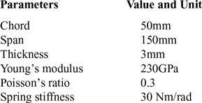
The sketch of the folded wing is shown in Fig. 1. If the inner and outer wings have the same mass and shape, then the length is 230 mm, the width is 100 mm, the thickness is 3 mm, 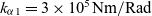 ${k_{\alpha 1}} = 3 \times {10^5}{\rm{Nm/Rad}}$,
 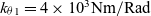 ${k_{\theta 1}} = 4 \times {10^3}{\rm{Nm/Rad}}$,
  ${\eta _{\alpha 1}} = 0$,
  ${\eta _{\theta 1}} = 120$, and the air density is
  $\rho = 1.224{\rm{kg/}}{{\rm{m}}^{\rm{3}}}$. Table 1 lists the simulation conditions for the deployment motion.
Table 1 Simulation conditions
4.1 Opening motion simulation analysis
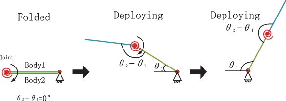
Figure 3 shows the deployment sequence, and also shows the timing diagram of the folding wing opening process, where the inner wing and outer wing are overlapped in the initial state. The deflection angle of the inner wing is defined as  ${\theta _1}$, and the deflection angle of the outer wing is defined as
  ${\theta _2}$. The deployment sequence is as follows. First, the system is in the initial state, the inner wing deflection angle is
  ${\theta _1} = 0^\circ $, the outer wing deflection angle is
  ${\theta _2} = 0^\circ $, and the relevant folding angle is
  ${\theta _2}{\rm{ - }}{\theta _1}$. Second, the inner wing rotates the system around the axis under the action of an impulse, and the outer wing rotates around the axis under the action of torsion spring and inertial force. Finally, when the two members are in the first parallel state, the action is terminated, and related folding angle
  ${\theta _2}{\rm{ - }}{\theta _1} = 180^\circ $.

Figure 3. Deployment sequence.
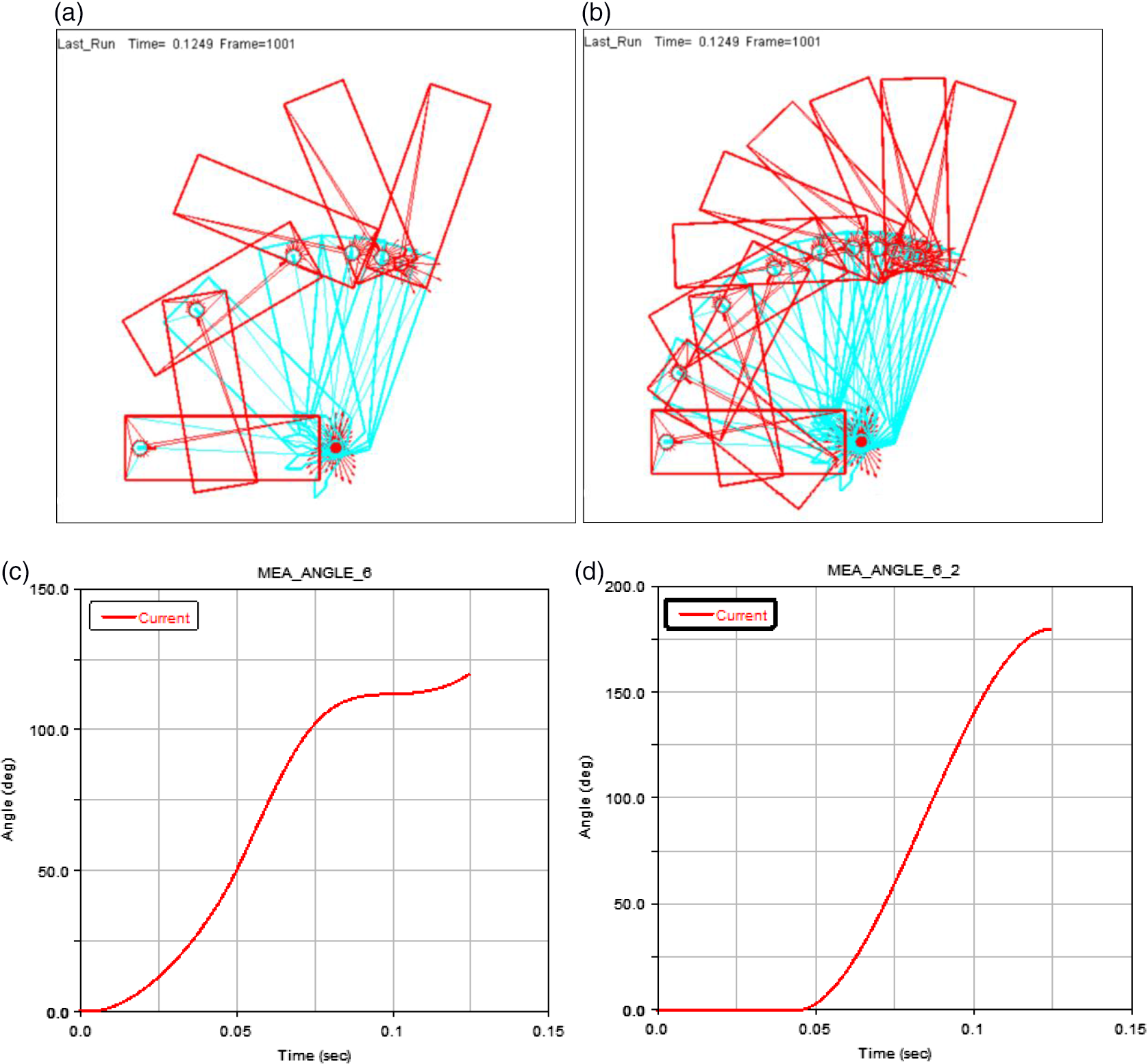
Figure 4. Folding wing motion system.(a)Folded wings low frequency expanded view,(b)High frequency expanded view of folded wings,(c)Folding angle of inner wing:  ${\theta _1}$,(d)Outer wing folding angle
  ${\theta _2}{\rm{ - }}{\theta _1}$.
Figure 4 shows the deployment motion simulation results after the rigid and aerodynamic models are decoupled, the spatial step size of the motion process is set to 1,101, and the time step size is 0.1249 s. Figure 4 (a) presents the schematic of a low-frequency-simulated motion sequence image. The image sequence has 6 frames, and each frame has a spatial step size of 200 and a time step of approximately 0.02s. Figure 4(b) presents the schematic of a high-frequency-simulated motion sequence image. The image sequence has 11 frames, and each frame has a spatial step size of 100, and the time step size is approximately 0.01 s. Both are 3D views of the entire deployment movement. Figure 4(c) shows that Angle1  $\left( {{\theta _1}} \right)$ starts to move from 0 and changes with time. No obvious change in the folding angle can be observed before 0.0042 s. This period is the process where the gunpowder begins to burn and produce gas to act on the piston, causing the piston to hit the inner wing. When the inner wing rotates through
  $119.5^\circ $, the inner wing is fully opened. Figure 4(d) shows that the relative folding angle
  $\left( {{\theta _2}{\rm{ - }}{\theta _1}} \right)$ also starts from 0 and changes with time. Initially, the two wings move together. After 0.044 s, the outer wing is separated from the inner wing under the action of torsion spring and inertial force. Unfolding exercises are performed. When the two wings coincide in a straight direction, that is,
  ${\theta _2}{\rm{ - }}{\theta _1} = 180^\circ $, the system is fully opened, indicating that the system ends the movement after 0.1249 s, and the type of aeroelastic response is sensitive to the initial conditions and the opening mode of the folded wing.
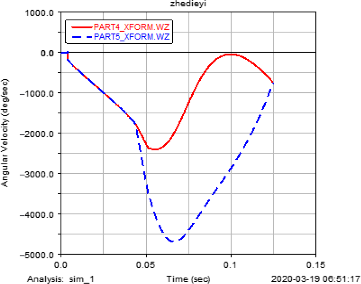
Figure 5. Folding wing angular velocity.
In the initial stage, the outer wing rotates around the  ${o_1}$ axis and moves in close contact with the inner wing. After 0.044 s, it expands and rotates around the
  ${o_2}$ axis, as shown in the following Fig. 5.
Figure 5 shows that the curve PART4 is the inner wing opening angular velocity, and the curve PART5 is the outer wing opening angular velocity. It also shows that before 0.0042 s, the system angular velocity is in the zero state. At 0.0042 s, the system starts to move, and the angular velocity is  ${\rm{ - }}190^\circ /{\rm{s}}$. Afterward, the two wings make rotational movements. At the termination time, the two wings have the same angular velocity. During the deformation process, a change in the type of motion is observed, and the aeroelastic response at certain folding corners may exhibit different types of motion.
Eq. (7) indicates that combined with the inner and outer wing folding angles ( ${\theta _1}$ and
  ${\theta _2}{\rm{ - }}{\theta _1}$) shown in Fig. 4, the coordinates of the centroids of wings
  ${c_1}$ and
  ${c_2}$ can be obtained, as shown in Fig. 6.
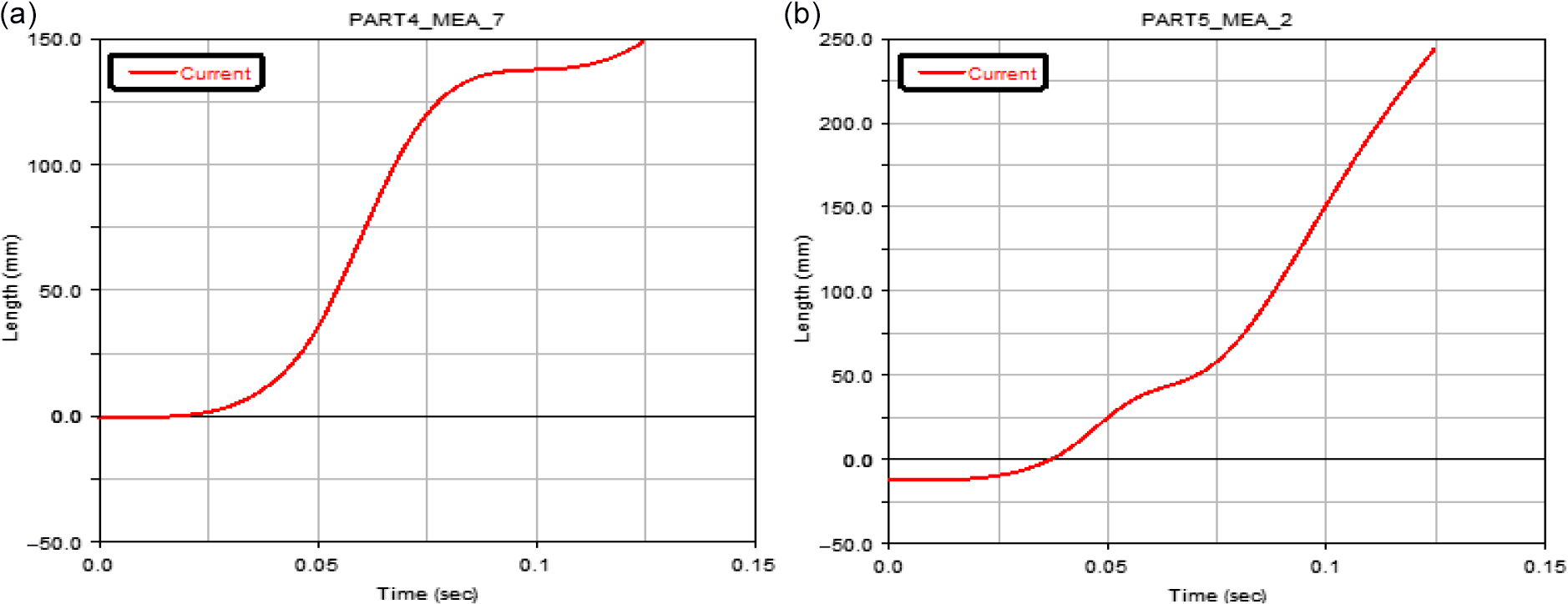
Figure 6. Folding wing coordinate system.(a)Inner wing centre of mass coordinates,(b)Outer wing centroid coordinates.
4.2 Vibration simulation analysis
After the dynamics and flutter analysis of the folding wing, the speed-time-curve graph is obtained, and the time-domain graph is converted into a frequency-domain graph, which can more intuitively observe the frequency distribution of vibration energy.
From the time domain to the frequency domain analysis, the abscissa is the frequency, and the data acquisition rate is 300Hz. The time domain function signal is converted into the corresponding amplitude at different frequencies by the fast Fourier transform (FFT). The characteristics of the frequency domain can more intuitively understand the frequency distribution of vibration energy when the folding wing is opened and grasp the vibration characteristics of the system. The analysis is carried out by the FFT graph. The upper graph is the speed-time function graph, and the lower graph is the frequency domain graph after fast Fourier transform. Figure 7 shows that the peak of the spectral density amplitude in the frequency characteristics of the inner wing’s x-direction speed occurs near 0 Hz, when the speed is  $1410{mm}/s^{2} $; Fig. 8 shows the frequency characteristics of the inner wing’s y-direction speed. The peak value of the amplitude occurs near 0Hz, and the speed is
  $827{mm} /{s^2}$ at this time. As the frequency increases, the speed gradually decreases; Fig. 9 shows the peak value of the spectral density amplitude in the frequency characteristics of the outer wing x-direction speed occurs at about 7.875Hz, at this time the speed is
  $1913{mm} {s^2}$, as the frequency increases, the speed gradually decreases; Fig. 10 shows that the peak of the spectral density amplitude in the frequency characteristics of the outer wing y-direction acceleration occurs near 0Hz, at this time, the speed is
  $3907{mm}/{s^2}$. Through the above analysis, it is found that all the vibration energy of the folding wing occurs at low frequencies. The vibration energy of the system is determined by the vibration state of the system. Due to the conservation of mechanical energy, the vibration energy of the folding wing system is determined by the initial state of vibration.
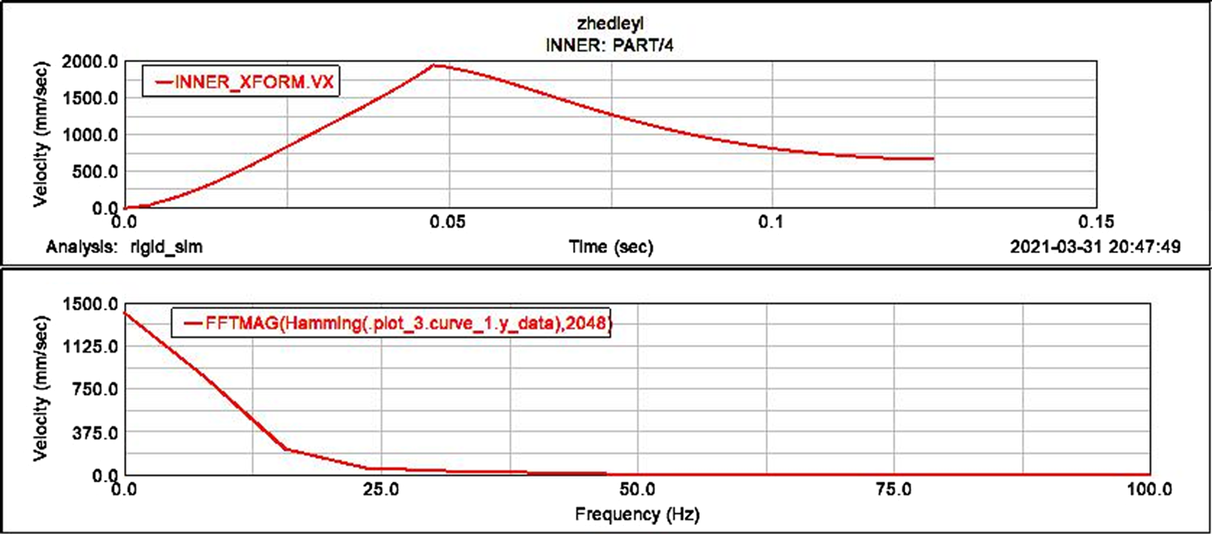
Figure 7. FFT curve of inner wing  $x{\rm{ - axis}}$ direction.
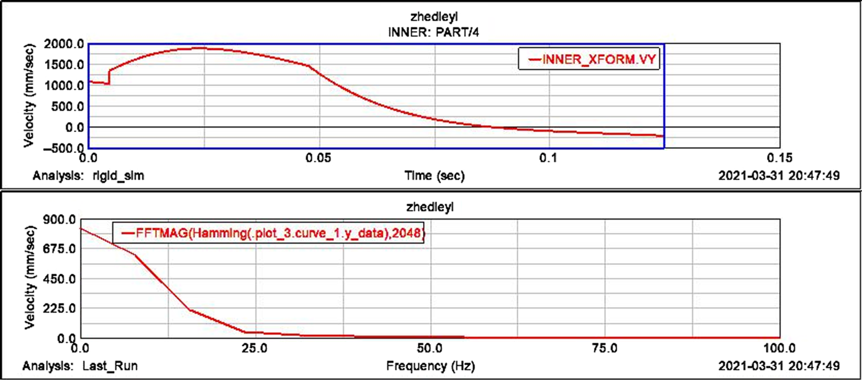
Figure 8. FFT curve of inner wing  $y{\rm{ - axis}}$ direction.
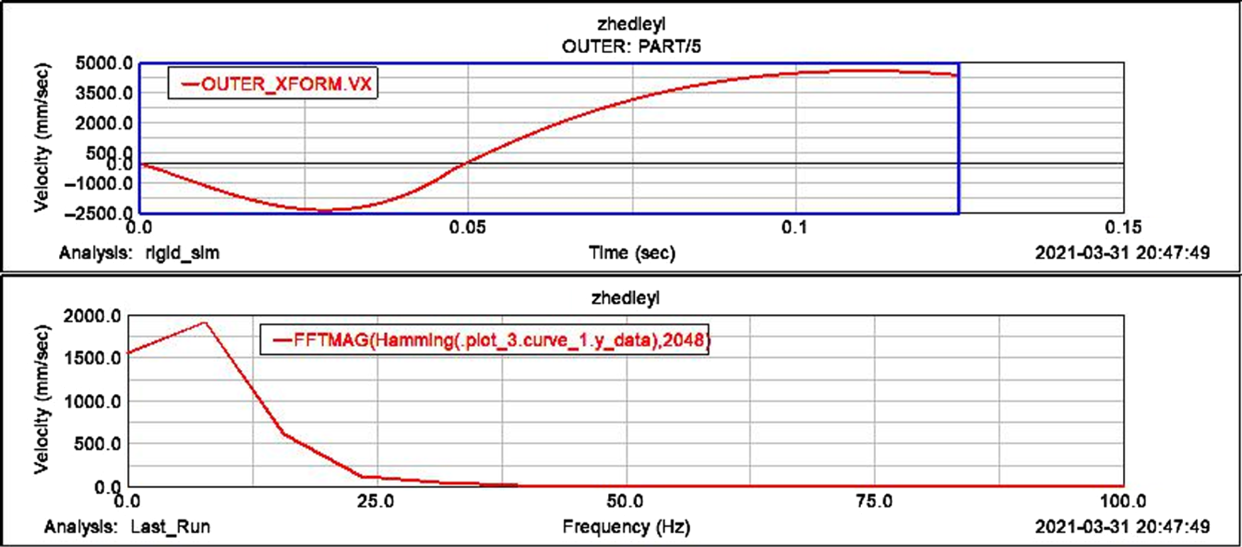
Figure 9. FFT curve of outer wing  $x{\rm{ - axis}}$ direction.
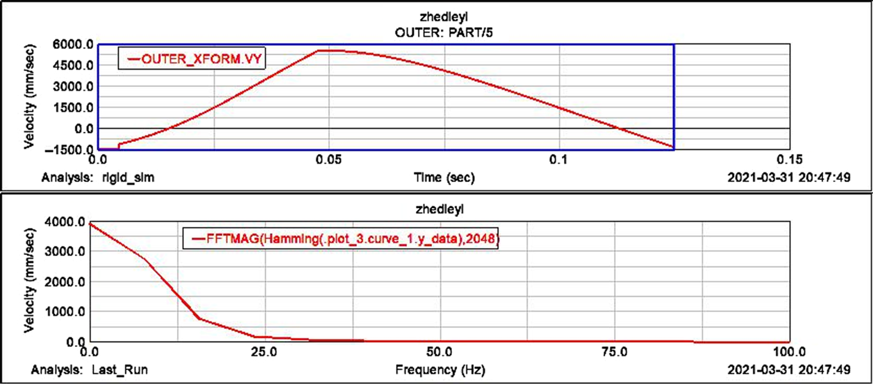
Figure 10. FFT curve of outer wing  $y{\rm{ - axis}}$ direction.
In order to analyse the amplitude of the folding wing during unfolding, at the beginning of the simulation, a vertical pulse excitation is applied to the edge point of the outer wing tail, then get the  $z$ -direction displacement response,
  $z$ -direction acceleration response and
  $z$-direction angular freedom response of a node of the inner and outer wings, as shown in the Figs. 11– 16.
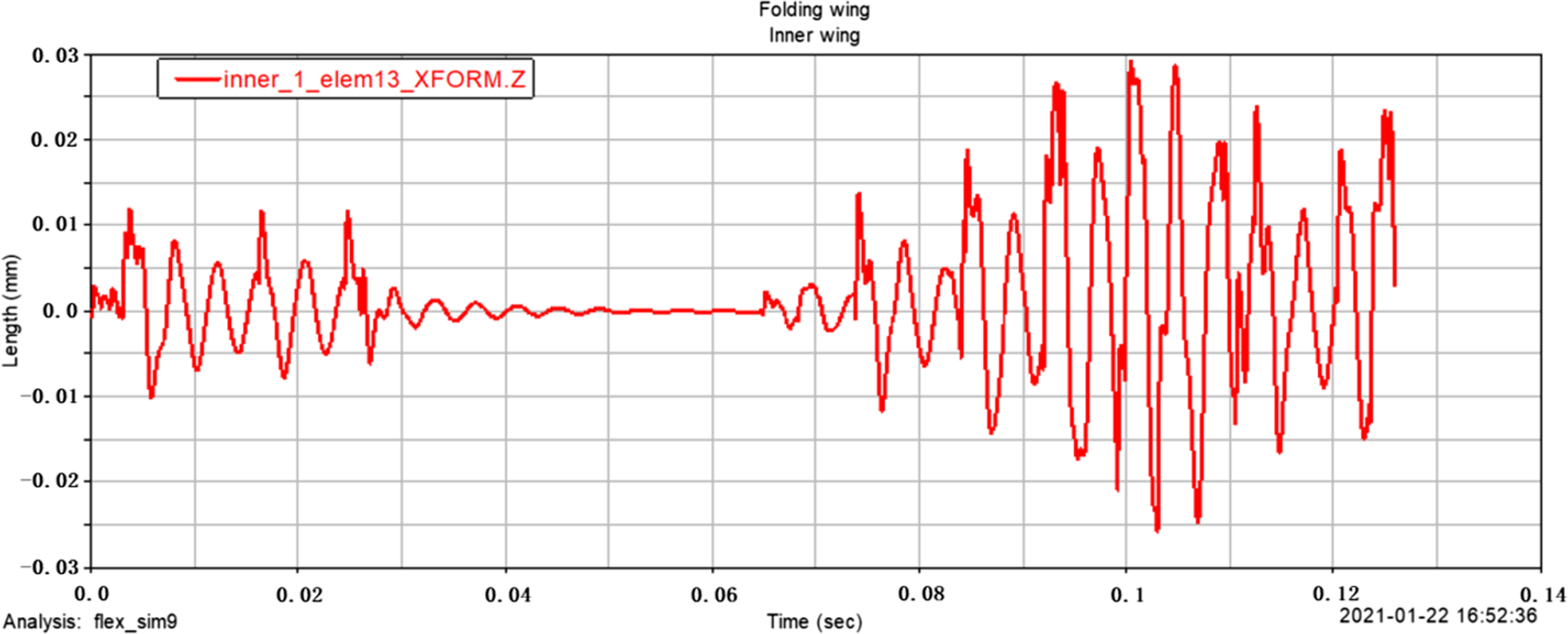
Figure 11. The  $z$ -direction displacement response of the inner wing centre of mass.
According to the analysis, the inner and outer wings show different characteristics under the action of excitation. Since the folding wing is a rigid-flexible coupling structure, and the wing is a flexible body, under the action of excitation, the displacement freedom and the angular freedom will all have a certain dynamic response. It can be seen from the comparison of Figs. 11 and 12 that the inner and outer wings show different displacement responses. The maximum z-direction displacement distance of the inner wing centre of mass is 0.03mm, and the maximum z-direction displacement distance of the outer wing centre of mass is close to 1.0E-004mm; from the comparison of Figs. 13 and 14, it can be seen that the maximum z-direction acceleration response of the inner wing centre of mass is close to 1.0E + 007mm/s2, and the maximum z-direction acceleration response of the outer wing centre of mass is close to 3500mm/s2, it can be seen that the amplitude and acceleration of the structure show a trend of simple harmonic change under the action of excitation. From the comparison of Figs. 15 and 16, it can be seen that the maximum z-direction angular freedom response of the inner wing centre of mass is about 0.065°, and the maximum z-direction angular freedom response of the outer wing centre of mass is about 2.25E-005°, the frequency of the z-direction angular degree of freedom response is unstable. This phenomenon-is caused by the change of the natural frequency of the folding wing structure with the folding angle. The results show that Adams software is feasible to simulate the displacement and forced vibration of the structure with simple harmonic excitation. The displacement and angular degrees of freedom of the structure are both small and can be ignored, so the opening motion has little influence. In addition, the amplitude variation curve of the folding wing with time, the z-direction acceleration curve of the wings centre of mass, and the degree of freedom response curve of the wings centre of mass, can provide references for the analysis of the unfolding motion characteristics of the folding wing.
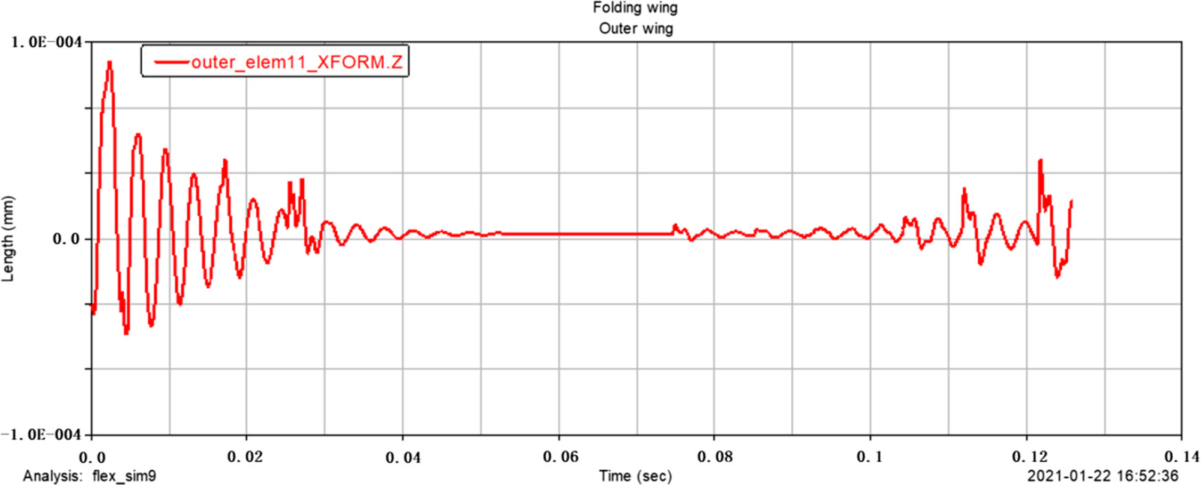
Figure 12. The  $z$ -direction displacement response of the outer wing centre of mass.
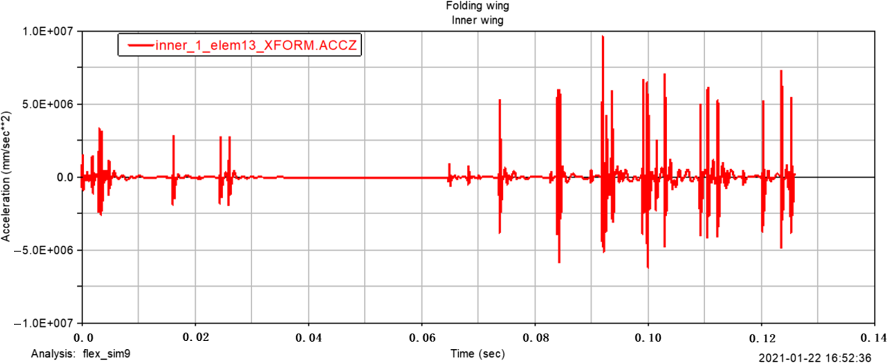
Figure 13. The  $z$ -direction acceleration response of the inner wing centre of mass.
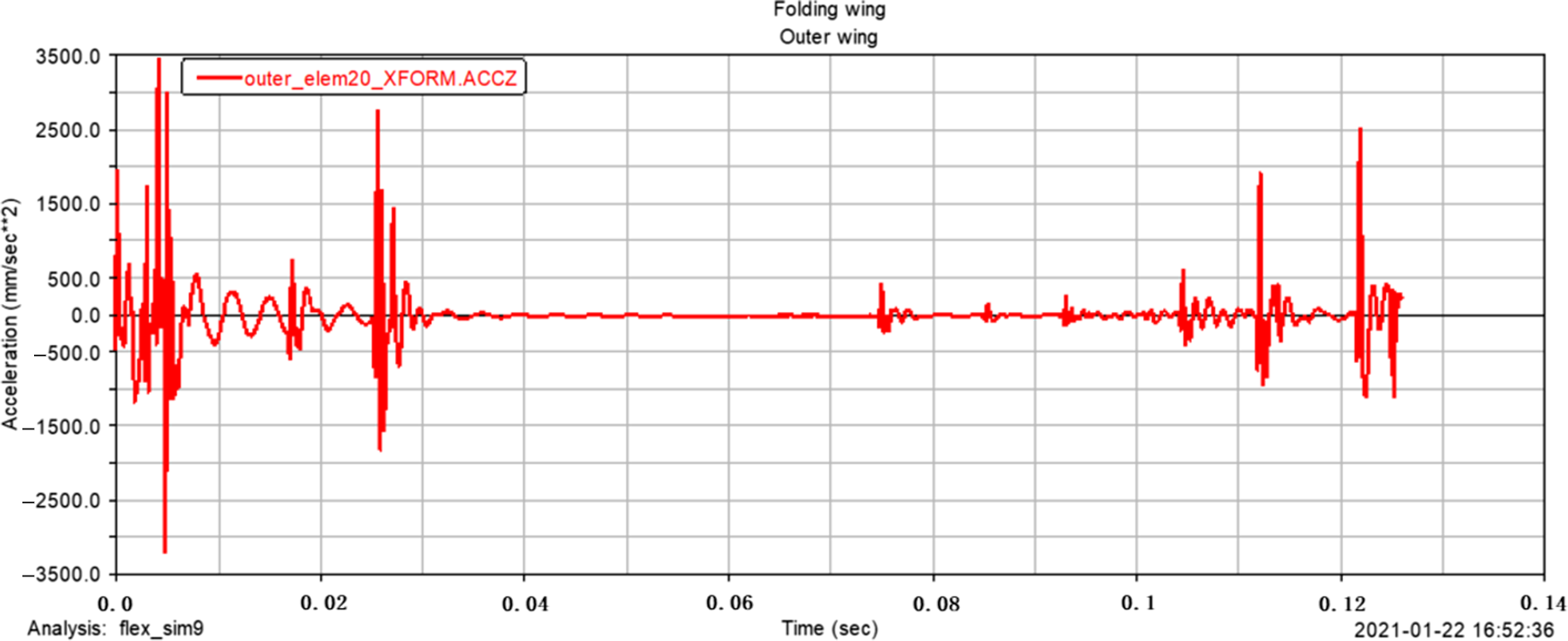
Figure 14. The  $z$ -direction acceleration response of the outer wing centre of mass.
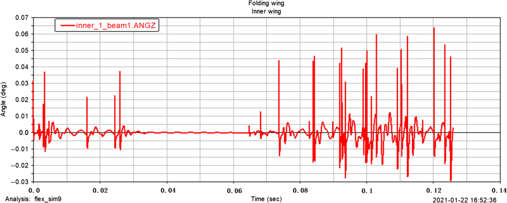
Figure 15. The  $z$ -direction angular freedom response of the inner wing centre of mass.

Figure 16. The  $z$ -direction angular freedom response of the outer wing centre of mass.
4.3 Analysis of aeroelastic properties
Flutter is a dynamic aeroelastic stability problem; as long as the appropriate aerodynamic theory is selected, flutter analysis can be performed. Flutter analysis is a double eigenvalue problem of frequency and speed, which is solved by the iterative method, and the assumed simple harmonic motion frequency reduction is used as the iterative parameter to obtain the moderately stable conditions (flutter frequency and speed) without artificial damping. In flutter analysis, the flutter solution can be easily expressed by a special frequency branch crossing the real axis. When the damping of the system passes through the  $x{\rm{ - axis}}$, the speed at this time is the critical speed — that is, the flutter critical speed — and the frequency corresponding to the critical speed is the flutter frequency.
Figure 17 shows the critical velocity diagram of a certain order of flutter in aerodynamic analysis under different folding angles. Finally, the flutter speed and frequency curves of the folding wings under different folding angles are drawn by the V-g and V-f methods.
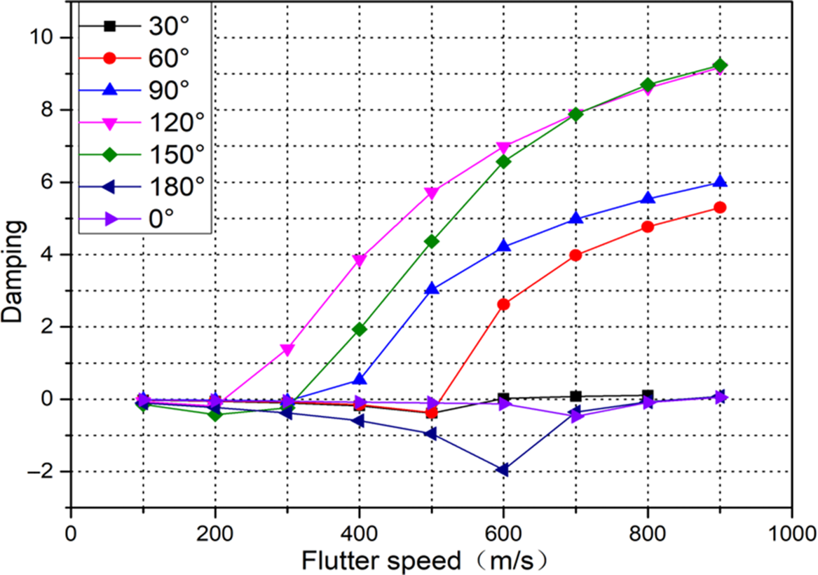
Figure 17. The relationship between flutter velocity and damping under different folding angles.

Figure 18. Flutter speed of folding wings at different folding angles.
Figures 18 and 19 respectively show the flutter speed and frequency obtained by MSC Nastran at different folding angles during the opening of the folding wings. Since there is a phase difference between the instantaneous aerodynamic force and the elastic displacement on the folding wing, the vibrating folding wing absorbs energy from the airflow to expand the displacement amplitude of a node of the folding wings. In addition to energy input, due to the instability of atmospheric environment, the relative flow of gases occurs, which causes the folding wing to vibrate. In the case of low speed, the energy absorbed by the folding wing will be consumed by damping without fluttering. Only when the speed exceeds at a certain value, chattering occurs.
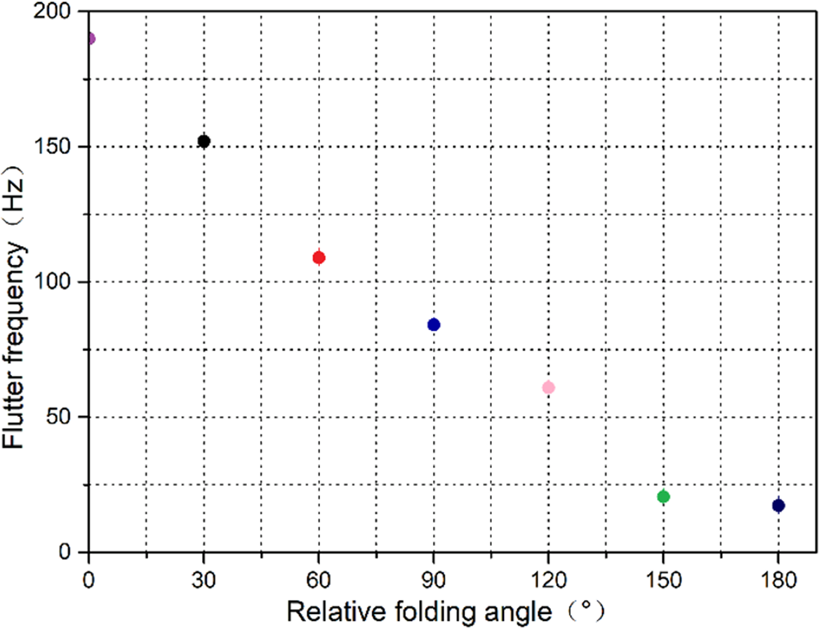
Figure 19. Flutter frequency of folding wings at different folding angles.
The comparison of the changes in the flutter characteristics of the models in Figs. 18 and 19 at different folding angles shows that when relative folding angle  ${\theta _2}{\rm{ - }}{\theta _1}$ changes between
  $0^\circ \sim 180^\circ $, the flutter velocity is between
 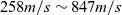 $258m/s \sim 847m/s$. When the relative folding angle changes between
  $0^\circ \sim 120^\circ $, the flutter speed decreases monotonously as the angle increases, and the flutter speed increases monotonously when the relative folding angle continues to increase to
  $180^\circ $. The flutter speed is the lowest when the relative folding angle is approximately
  $120^\circ $, that is, approximately
  $258m/s$, and the flutter speed is the highest when the relative folding angle is about
  $180^\circ $, that is, approximately
  $847m/s$. Therefore, when the folding wing is fully opened, its critical flutter velocity is 847 m/s. Analysis shows that due to the uncertainty of the atmospheric environment, the aeroelastic system of the folding wing will appear stable and unstable, respectively; flutter frequency and speed have different trends and show a monotonous decreasing trend as the relative folding angle increases.
4.4 Physical experiment verification
The physical model of the folded wing is placed on the test bench. The inner wing passes through a vertical metal shaft. The model material is aluminum alloy. If the main charge is 2/1 camphor single-base propellant, the inner theoretical peak of the bore pressure of the main charge of  $200mg$ introduced by the ballistic program is about
  $10MPa$, the cross-sectional area of the piston is
  $100m{m^2}$, and the starting pressure of the piston end is about
  $1000N$, which will be offset by friction during the movement of the piston. A part of the force is applied to the impact of the inner wing, and the folding wing will rotate and open around the axis.
As shown in Fig. 20, (a) is the timing diagram of dynamic simulation, and (b) is the timing diagram of physical model experiment. The simulation and experiment process are divided into four time sequences. When the simulation and experiment are the same time sequence, the wing is folded. The corresponding positions are roughly the same. Because the physical model is placed on a static vertical axis, all external factors such as the actual flight speed and rotation speed of the projectile are not considered, which makes the result deviate from the simulation, but it can be proved that the folding wings can be rotated and opened.

Figure 20. Sequence diagram of simulation and experiment.
5.0 CONCLUSIONS
In the process of opening the folding wing, the structural model of the longitudinal double-folding wing was established by using Lagrange equation, and the kinematic characteristics of the multi-body motion were analysed, and the dynamic model of the folding wing in the impact ejection stage was constructed using a dipole. The grid method was used to calculate the generalised unsteady aerodynamic force, the aerodynamic model was converted into the time domain by the minimum state method, and the aerodynamic model was converted into the time domain dynamic model by the rational number function approximation. Finally, the aeroelastic equation of the folded wing was obtained.
Meanwhile, the opening angular velocity required during the movement of the folding wing under a certain impulse was analysed, and the 3D sequence image of the opening movement of the folding wing was obtained through the kinematic equation simulation. The opening angle and the centroid position of the inner and outer wings were obtained, the vibration energy of the folding wing system is determined by the initial state of the vibration, the law of time changes, aeroelastic analysis was performed on the folding wing under different relative folding angles, and the change trend of the flutter speed and frequency was obtained. The results show that due to the uncertainty of the atmospheric environment and the changes in missile flight speed and folding wing opening speed, the aeroelastic system of the folding wing will appear stable and unstable, respectively. The aeroelastic response is not only sensitive to initial conditions, but also the folding angle. Therefore, when designing the folding wing system, it is necessary to choose the power source for the initial opening of the folding wing to ensure that the folding wing is opened quickly within a certain period of time.
ACKNOWLEDGMENTS
We would like to thank KGSupport (http://www.kgsupport.com/) for its linguistic assistance during the preparation of this manuscript.
CONFLICT OF INTEREST STATEMENT
There is no conflict of interest.
DATA AVAILABILITY
Some or all data, models, or code that support the findings of this study are available from the corresponding author upon reasonable request.
SUPPLEMENTARY MATERIAL
To view supplementary material for this article, please visit https://doi.org/10.1017/aer.2021.52