Nomenclature
- α
angle-of-attack, deg
- δ e
elevator deflection, deg
- c
chord, m
- C D
drag force coefficient
- C L
lift force coefficient
- C m
pitching moment coefficient
- C X
axial force coefficient
- C Z
normal force moment coefficient
- e
Oswald efficiency factor
- F eng
thrust force, N
- I X
moment of inertia along X-axis, kg m2
- I Y
moment of inertia along Y-axis, kg m2
- I Z
moment of inertia along Z-axis, kg m2
- I XZ
moment of inertia along XZ-axis, kg m2
- p
roll rate, deg/s
- q
pitch rate, deg/s
-
 $${\rm _\dot{q}}$$
pitch acceleration, deg/s2
- r
yaw rate, deg/s
- V
relative total airspeed, m/s
- σt
thrust inclination angle, deg
- θ
vectors of unknown parameters
- α*
breakpoint, deg
- τ1,τ2
transient and hysteresis time constants, respectively, s
- ε
distributed noise
- AR
aspect ratio
- GP
Gaussian process

1.0 INTRODUCTION
High fidelity aerodynamic models are increasingly in demand for applications such as flight control, simulation, aerodynamic database development, and fault detection and diagnosis. These aerodynamic models are usually extracted from the wind tunnel test measured data( Reference Grauer and Morelli 1 ). Developing an aerodynamic model using wind tunnel data has some limitations. To get the efficient model, it needs sizeable aerodynamic database using wide ranges of flight envelope with high-resolution data acquisition especially, for non-linear aerodynamic modelling. It demands enormous amounts of time, money, computational resources, and manpower. Further, the acquired model needs to be corrected for boundary layer, Reynolds number, and scaling effects. Various other sources of error can make the aerodynamic coefficient erroneous and discontinuous. This also leads to issues in computing gradients for optimisation, control analysis, trimming, and generating linear models. Wind tunnel generated databases also face challenges in gaining physical insights( Reference Grauer and Morelli 1 – Reference Morelli Eugene 5 ).
Aerodynamic modelling from the alternate method, using flight test data, is an efficient way to model the aircraft behaviour which overcomes most of the challenges mentioned in wind tunnel-based methods. Flight data generally, capture complete aircraft behaviour which can be used in model postulation and also for aerodynamic parameter estimation. Aerodynamic parameter estimation is a process of identifying the parameter associated with the model. These parameters are generally obtained by minimising the error between the model and the plant. This is also known as an output error method for parameter estimation. Maximum-likelihood estimation (MLE) is one such method under this category. A classical method based on MLE has been extensively used to estimate the parameters from high angle-of-attack flight data. Aerodynamic modelling at a high angle-of-attack makes aircraft to enter in the non-linear regime, which is cumbersome to model using traditional parametric methods( Reference Jategaonkar 2 – Reference Morelli 6 ).
Non-linear aerodynamic modelling from high angle-of-attack flight data has been studied from several decades by various research labs across the globe. Goman and Khrabrov( Reference Goman and Khrabrov 7 ) proposed a state space approach for unsteady aerodynamic forces and moments model. Nelson and Pelletier( Reference Nelson and Pelletier 8 ) have reviewed preliminary information on the flow structure over delta wings and complete aircraft configurations. Fischenberg and Jategaonkar( Reference Fischenberg and Jategaonkar 9 ) have demonstrated the quasi-steady stall modelling and also parameter estimation on C-160 transport aircraft. Ghoreyshi and Cummings( Reference Ghoreyshi and Cummings 10 ) have presented a time-dependent surrogate approach to capturing the unsteady aerodynamics for various manoeuvers. However, in current findings, neural-based methods have been extensively used for this purpose. Neural Gauss–Newton (NGN)-based methods were developed by Peyada and Ghosh( Reference Peyada and Ghosh 11 ) for the low angle-of-attack flight modelling, and by Kumar and Ghosh( Reference Kumar and Ghosh 12 , Reference Kumar and Ghosh 13 ) further, it was attempted on non-linear aerodynamic modelling. Faller and Schreck( Reference Faller and Schreck 14 ) proposed a recurrent multilayer perceptron neural network (MLP-NN) for the aerodynamic derivative identification. Marques and Anderson( Reference Marques and Anderson 15 ) applied a multi-layer-based temporal neural network to estimate unsteady aerodynamics of transonic flow. Consequently, Voitcu and Wong( Reference Voitcu and Wong 16 ) demonstrated the suitability of a neural network for modelling and dynamic behaviour of an aeroelastic system. Further, Zhang et al.( Reference Zhang 17 ) and Winter and Breitsamter( Reference Winter and Breitsamter 18 ) employed radial basis function neural network (RBF-NN) for the accurate modelling of unsteady aerodynamic force coefficients in transonic flow. Moreover, some combinations of the system identification methods with the POD-based approaches have been published. Within an aeroelastic optimisation framework, recently a successful combination of Zhang’s RBF-based non-linear system identification approach with the POD-based non-linear system identification approach with the POD has been proposed by Lindhorst et al.( Reference Lindhorst, Haupt and Horst 19 ). A surrogated modelling approach comparable to the method of Lindhorst et al. is proposed by Winter and Breitsamter( Reference Winter and Breitsamter 20 ). Another technique used for modelling the aerodynamics of non-linear regime is modelling using multivariate functions( Reference Winter and Breitsamter 20 ). Neural network-based methods have been quite frequently used to develop aerodynamic modelling, which has provided decent results. However, due to the hidden layer of the neural network sometimes, it leads to computational complexity and instability in numerical solutions. There is a lack of detailed methodology on the selection of the number of hidden units and its architecture. Another issue that users may face is a long training time, which often causes an issue in the convergence( Reference Babuska 21 – Reference Chati and Balakrishnan 28 ).
This paper is an attempt to get a non-parametric probabilistic model using Gaussian process regression (GPR) approach. This is a machine learning-based data-driven approach which deals with the measured flight dataset. GPR is a function approximation as a distribution over functions. Any true function in the domain defines in the Gaussian distribution by modelling their evaluated mean and covariance functions. GPs are used in various disciplines for which underlying functions are unknown. A GP can be implemented as the regression of training data with respect to a basis function. Data analytics and machine learning community have applied GP to both controls and estimation processes. GP can be used to learn the unknown dynamic and measurement model. In the implementation of GP, statistical mean infers the approximate of the state transition matrix and measurement model, while the statistical covariance estimates the process and measurement white noise( Reference Lee and Johnson 29 – Reference Saderla, Dhayalan and Ghosh 32 ).
Machine learning algorithms offer a powerful tool to achieve a data-driven model. In this paper, we use GPR, to model the aerodynamic force and moment coefficients: lift force coefficient (C L), drag force coefficient (C D), and pitching moment coefficient (C m) using the measured flight data from DLR-ATTAS aircraft( Reference Jategaonkar 2 ). Open accessible flight test data of ATTAS research aircraft from DLR, Germany were used in the estimation and validation of the aircraft lift, drag, and pitching moment coefficients. Flight test data were segregated as input and output data set. Input data were sets of the angle-of-attack, elevator deflection, pitch rate, and relative airspeed; output data were sets of measured force and moment coefficients. Non-linear model estimation was carried out using a kernel-based probabilistic model known as GPR. Further, an exponential squared function was chosen judiciously to use as a kernel function. GPR model was trained and validated with real flight data. Seventy per cent of the data were used in training, and the remaining 30% of the data were used for the validation of the model. Statistical modelling technique was used in quantifying the uncertainty in the model. GPR models were found to give mean errors of 2.7%, 0.8%, and 0.5% in the coefficients of lift force, drag force, and pitching moment, respectively. GPR estimated non-linear aerodynamic models were compared with MLE-predicted models. MLE methods have been a popular classical method for several decades. Estimated results from both the methods GPR and MLE were found to be in close agreement with each other. GPR estimated C L and C D were reasonably close to MLE-estimated results. The estimation of C m using GPR was highly efficient which is corroborated by the correlation analysis. Presented results proved to make GPR as a promising alternative approach to this problem. GPR does not require to solve the equation of motion, this advantage further motivates promising directions for future research and can be readily generalised to other applications such as aeroelasticity, load estimation, and optimisation.
This paper has the following contributions:
(1) Development of a probabilistic model for lift force, drag force, and pitching moment coefficient with GPR.
(2) Statistical comparison with conventional method MLE using a quasi-stall modelling approach.
The organisation of the paper is structured as follows: Section 2.0 presents the GPR methodology and the formulation of the algorithm; Section 3.0 explains the non-linear aerodynamic modelling using MLE-based parametric model approach; Section 4.0 presents results and discussion of estimated models. Conclusions are summarised in Section 5.0.
2.0 METHODOLOGY: GPR
GPR is a robust non-parametric tool for learning regression functions from the observed input–output dataset. It is based on a Bayesian approach with a Gaussian probabilistic framework( Reference Chati and Balakrishnan 28 ). A regression model is given as
 $$y{\rm }{\equals}{\rm }g(x){\rm }{\plus}{\rm \epsilon}$$
where y is the output/dependent variable which contains flight variable derived lift force coefficient (C L), drag force coefficient (C D), and pitching moment coefficient (C m). x is the input vector containing: angle-of-attack (α), elevator deflection (δe), pitch rate (q), and relative airspeed (V). g(x) is the regression function and ϵ is the distributed process noise. For inputs x following a joint Gaussian distribution, function g(x) is said to follow a Gaussian process( Reference Lee and Johnson 29 ):
 $$g{\rm (}x{\rm )\colon\,GP(}m_{{\rm e}} {\rm (}x{\rm ),}\,T{\rm (}x{\rm ,\,}x'{\rm ))}$$
where m
e(x) is the mean function and T(x, x′) is the kernel function over two inputs x and x′, which governs the covariance among function values. In this work, mean function is assumed to be the zero function. Generally, noise is assumed to follow a Gaussian distribution,
 $${\rm {\epsilon}}\,\sim\,{N}{\rm (0,\rsigma }_{{n}}^{{\rm 2}} {\rm )}$$
, with mean 0 and noise variance
$${\rm {\epsilon}}\,\sim\,{N}{\rm (0,\rsigma }_{{n}}^{{\rm 2}} {\rm )}$$
, with mean 0 and noise variance
 $${\rm \rsigma }_{n}^{2} $$
. For the assumption of a zero mean function for the GP governing the regression function and Gaussian noise, the dependent variable y also follows a GP with a zero mean function and a ‘noisy’ kernel function T
noise(x
l, x
m) over d-dimensional input vectors x
l and x
m:
$${\rm \rsigma }_{n}^{2} $$
. For the assumption of a zero mean function for the GP governing the regression function and Gaussian noise, the dependent variable y also follows a GP with a zero mean function and a ‘noisy’ kernel function T
noise(x
l, x
m) over d-dimensional input vectors x
l and x
m:
 $$y\,\sim\,{\rm GP(0,}\,T_{{{\rm noise}}} {\rm (}x_{\rm l} {\rm ,}\,x_{\rm m} {\rm ))}$$
The noisy kernel function over the dependent variables T noise(x l, x m) relates to the kernel function over the regression function values k(x p, x q) as
 $$T_{{{\rm noise}}} {\rm (}x_{\rm l} {\rm ,\,}x_{\rm m} {\rm ) {\equals} }T{\rm (}x_{\rm l} {\rm ,\,}x_{\rm m} {\rm ) {\plus} \rsigma }_{{\rm n}}^{{\rm 2}} {\rdelta }_{{{\rm l m}}} $$
where δ is the Kronecker delta.
GP can employ various kernel functions to affect the regression models which enables its flexibility( Reference Lee and Johnson 29 ). In this work, the squared exponential kernel function is used to train the regression model.
2.1 Dot Product Squared Exponential (DPSE) kernel
This kernel function is used to model very smooth functions. It is given by
 $$\eqalignno{ & T{\rm (}x_{\rm l} {\rm ,}\,x_{\rm m} {\rm ){\equals}{\rsigma }_{0}^{2} {\rm {\plus}}}x_{\rm l}^{\rm T} \Sigma x_{\rm m} {\plus}{\rm \rsigma }_{f}^{2} \,{\rm exp}\left( {{\minus}{1 \over 2}\mathop{\sum}\limits_{i{\equals}1}^d {{{(x_{{\rm l,i}} {\minus}x_{{\rm m,i}} )^{2} } \over {p^{2} }}} } \right), \cr & \Sigma {\equals}{\rm diag}({\rm \rsigma }_{1}^{2} ,{\rm \rsigma }_{2}^{2} ,...,{\rm \rsigma }_{d}^{2} ) $$
In Eq. (5), x
l and x
m are d-dimensional input column vectors,
 $${\rm \rsigma }_{0}^{2} $$
is the constant variance parameter,
$${\rm \rsigma }_{0}^{2} $$
is the constant variance parameter,
 $${\rm \rsigma }_{1}^{2} ,{\rm \rsigma }_{2}^{2} ,...,{\rm \rsigma }_{d}^{2} $$
are the variance parameters corresponding d input dimensions,
$${\rm \rsigma }_{1}^{2} ,{\rm \rsigma }_{2}^{2} ,...,{\rm \rsigma }_{d}^{2} $$
are the variance parameters corresponding d input dimensions,
 $${\rm \rsigma }_{f}^{2} $$
is a variance parameter which governs the exponential part of the kernel, p is the d-dimensional vector of length scales, i refers to the ith vector component. Kernel parameters are generally called as hyperparameters. Hyperparameters for the above GPR formulation can be written as
$${\rm \rsigma }_{f}^{2} $$
is a variance parameter which governs the exponential part of the kernel, p is the d-dimensional vector of length scales, i refers to the ith vector component. Kernel parameters are generally called as hyperparameters. Hyperparameters for the above GPR formulation can be written as
 $$\hskip 128pt{\rm [\rsigma }_{0}^{2} ,{\rm \rsigma }_{1}^{2} ,{\rm \rsigma }_{2}^{2} ,...,{\rm \rsigma }_{d}^{2} ,{\rm \rsigma }_{d}^{2} ,p]^{{\rm T}} $$
…(6)
$$\hskip 128pt{\rm [\rsigma }_{0}^{2} ,{\rm \rsigma }_{1}^{2} ,{\rm \rsigma }_{2}^{2} ,...,{\rm \rsigma }_{d}^{2} ,{\rm \rsigma }_{d}^{2} ,p]^{{\rm T}} $$
…(6)
The noisy kernel hyperparameter vector is characterised by the noise variance
 $${\rm \rsigma }_{n}^{2} $$
. The vector which maximises the log posterior probability of the hyperparameter vector for given of input vectors X and of dependent variable values y are known as the estimated vector
$${\rm \rsigma }_{n}^{2} $$
. The vector which maximises the log posterior probability of the hyperparameter vector for given of input vectors X and of dependent variable values y are known as the estimated vector
 $$\eqalignno{ & {\rm \vskip-5pt \hat \hskip-17pt \;\;\vskip}{{\rtheta } & {\equals}} \mathop{{{\rm argmax}}}\limits_{{\rm \rtheta }} \,\log q({\rm \rtheta }\mid X,y) \cr & \hskip-6.5pt{\rm {\equals} }\mathop{{{\rm argmax}}}\limits_{{\rm \rtheta }} \,\log \left\{ {q({\rm \rtheta }){\minus}{1 \over 2}y^{T} K_{Y}^{{{\minus}1}} y\,\,{\minus}{1 \over 2}\log \left| {K_{y} } \right|{\minus}{n \over 2}\log (2{\rm \rpi })} \right\} $$
here, q(θ) is the prior on the hyperparameter vector, n is the number of observations, X is the n × d matrix of d-dimensional inputs, y is the n × 1 vector of the dependent variable C L, C D, or C m values, and Ky is the n × n covariance matrix derived from the noisy kernel function over pairs of input variables.
In this paper, the GPR model aims to predict force and moment coefficients on new input data sets. GPR methodology has many advantages: (a) it is a non-parametric method, which makes user free from choosing basis function prior to training, (b) it maintains a probabilistic framework based on the Gaussian distribution which makes the analysis tractable, and (c) it is possible in GPR to determine the full predictive distribution which proves to be useful product of the analysis( Reference Lee and Johnson 29 – Reference Saderla, Dhayalan and Ghosh 32 ).
3.0 NON-LINEAR AERODYNAMIC MODELLING USING PARAMETRIC MODEL APPROACH
This section describes the non-linear aerodynamic modelling of DLR-ATTAS aircraft based on the MLE method. MLE is an output error-based parametric modelling approach. The output error between model and plant is minimised by the Gauss–Newton optimisation method. The model adopted in this method is quasi-steady stall model( Reference Jategaonkar 2 , Reference Kumar and Ghosh 12 ).
3.1 Quasi-steady-stall modelling
Near stall flight data of DLR-ATTAS are selected for non-linear aerodynamic model estimation. MLE uses the following Kirchhoff’s quasi-steady stall model( Reference Jategaonkar 2 ) as shown in the following equation:
 $$\eqalignno{ C_{{\rm L}} ({\ralpha ,}\,\,X{\rm )} & {\equals}C_{{L_{0} }} {\plus}C_{{{\rm L}_\ralpha }} \left\{ {{{{\rm 1{\plus}}\sqrt X } \over {\rm 2}}} \right\}^{2} {\ralpha } \cr C_{{\rm D}} & {\equals}C_{{\rm D}} _{{_{_0} }} {\plus}{1 \over {e{\rm \rpi AR}}}\,C_{{\rm L}} ^{2} \left( {{\ralpha ,\,}X{\rm ,\,}q{,\,\rdelta }_{\rm e} } \right){\plus}C_{{\rm D}{_X} } (1{\minus}X) \cr C_{{\rm m}} & {\equals}C_{{\rm m}} {{_{_0} }} {\plus}C_{{{\rm m}_{\ralpha } }} {\ralpha }{\plus}C_{{{\rm m}_{q} }} {{q\overline{c} } \over {2V}}{\plus}C_{{\rm m_x}} (1{\minus}X) $$
The flow separation point in the above equations is estimated using the following equation:
 $${\rm \rtau }_{{\rm 1}} {{{\rm d}X} \over {{\rm d}t}}{\rm {\plus}}X{\rm {\equals}}{{\rm 1} \over {\rm 2}}\left\{ {{\rm 1\minus}\tanh \left[ {a_{{\rm 1}} \left( {{\ralpha }{\,\minus\,}{\rm \rtau }_{{\rm 2}} {\rm {\ralpha {\hskip-4pt\vskip-3pt\cdot}}}{\,\minus\,}{\ralpha {^\asterisk}}} \right)} \right]} \right\}$$
where a 1 is aerofoil static stall characteristics, τ2 is the time constant and α* is the breakpoint. These three parameters are adequate to capture stall hysteresis( Reference Jategaonkar 2 ). Generally, aerodynamic forces and moment coefficients (C L, C D, C m) are not directly measured during flight; these are derived from the other measured flight variables such as flow angles, accelerations. These coefficients have been reconstructed from the measured accelerations and flow angles and mass inertia parameters. The following θstall vector is a set of aerodynamic and stall parameters which are estimated by minimising the output error:
 $${\rtheta }_{{{\rm stall}}} {\rm {\equals}}\left[ {{\rm C}_{{{\rm D}_{0} }} {\,\rm e C}_{{{\rm L}_{0} }} {\rm C}_{{{\rm L}_{\ralpha } }} {\rm C}_{{{\rm L}_{{\ralpha _{{M\ralpha }} }} }} {\rm C}_{{{\rm m}_{0} }} {\rm C}_{{{\rm m}_{\ralpha } }} {\rm C}_{{{\rm m}_{q} {\rm }}} {\rm C}_{{{\rm m}_{{\rdelta \rm e}} {\rm }}} {\rm a}_{{\rm 1}} {\rm \ralpha {^\asterisk} \rtau }_{{\rm 2}} {\rm C}_{{{\rm D}_{X} }} {\rm C}_{{{\rm m}_{X} }} } \right]^{{\rm T}} $$
These parameters are estimated using output error based MLE method.
3.2 MLE Method
MLE is a powerful estimation tool for parameter estimation. It estimates the parameters by minimising the output error between the measured and model response. This is an effective method for aircraft parameter estimation. MLE uses the postulated quasi-steady stall model described in the above section. This works well even in the case of measurement noise. However, it faces a convergence issue for some of the application( Reference Jategaonkar 2 – Reference Mehra, Stepner and Tyler 4 ).
The accuracy in MLE estimates is quantified by Cramer–Rao bounds (CRB). The cost function used in this method is shown in the following equation:
 $$J{\rm (\rtheta ){\equals}}{{\rm 1} \over {\rm 2}}\mathop{\sum}\limits_{k{\rm {\equals}1}}^N {\left\{ {\left[ {Z_{{t{\rm (}k{\rm )}}} {\,\minus}\,Z_{{{\rm \rtheta ,\it t(}k{\rm )}}} } \right]^{{\rm T}} \left( {\rm UU^{{\rm T}} } \right)^{{{\minus}{\rm 1}}} \left[ {Z_{{t{\rm (}k{\rm )}}} {\minus}Z_{{{\rm \rtheta ,}t{\rm (}k{\rm )}}} } \right]} \right\}} $$
where N is the number of time data points, UUT is the measurement noise covariance matrix, Z t(k) is the measure response at kth instant, and Z θ,t(k) =estimated response for given θ vector at kth instant.
Further, the MLE detail description can be understood by Refs Reference Jategaonkar2–Reference Mehra, Stepner and Tyler4. The implementation of MLE has been discussed in the results and discussion section.
4.0 RESULTS AND DISCUSSION
Open accessible flight test data of the research aircraft DLR-ATTAS has been in the estimation of the aircraft lift, drag, and pitching moment coefficientsReference Jategaonkar (2) and demonstrated the efficacy GPR algorithm for the non-linear aerodynamic modelling from the flight data.
4.1 Non-linear modelling using GPR
In this paper, GPR-based method has been employed for the non-linear aerodynamic modelling. The efficacy of this novel approach is demonstrated on the DLR-ATTAS quasi-steady stall data for the force and moment coefficient modelling. Seventy per cent of the flight test data has been used for the training, and the remaining 30 percent of the data has been used for the validation. A kernel-based probabilistic function is used as a covariance function in designing the GPR model [33] .
Data used in GPR are presented in Fig. 1 with time history. Data have been acquired at 25 Hz. Elevator deflection affects other aircraft variables which are observed in the figure. Elevator was deflected by around 8° in both the directions. Change in a x and a z are significant. An angle-of-attack varies between +18 and −18°. Change in theta is around 15°. Change in q is between −4 dps and +4 dps.
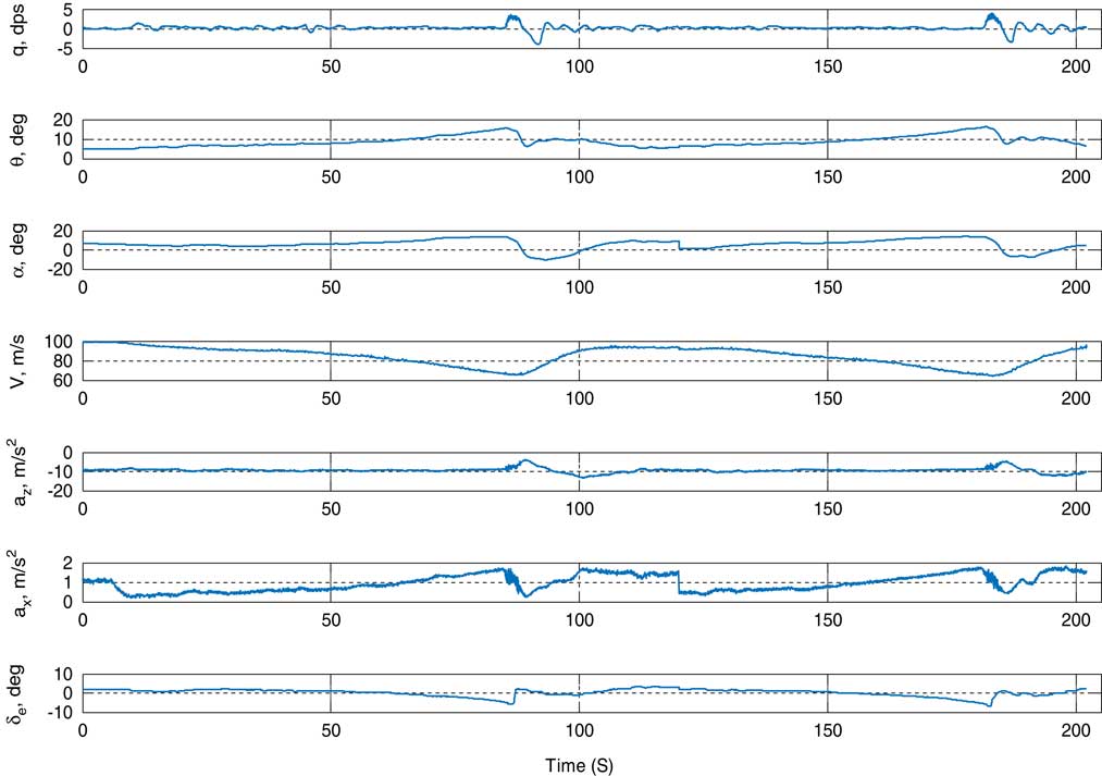
Figure 1 (Colour online) Time history plot for ATTAS quasi-stall data.
In the presented work, coefficients of the lift force, drag force, and pitching moment were estimated using GPR and compared with the MLE estimated results. Dataset chosen for the implementation of GPR and MLE were segregated as input and output dataset. Input data were categorised with the angle-of-attack, elevator control surface deflection, pitch rate, and relation airspeed. Output data were categorised with force and moment coefficients.
Figure 2 shows the GPR-predicted model for the coefficient of the lift force, the coefficient of the drag force and the coefficient of the pitching moment. GPR-predicted coefficients are matching well with the measured coefficients. The correlation of GPR predicted coefficient of the lift force, the coefficient of the drag force, and coefficient of the pitching moment coefficient with the measured data were found to be 0.95, 0.99, and 0.91, respectively. The statistical result shows the confidence in the GPR predicted model.
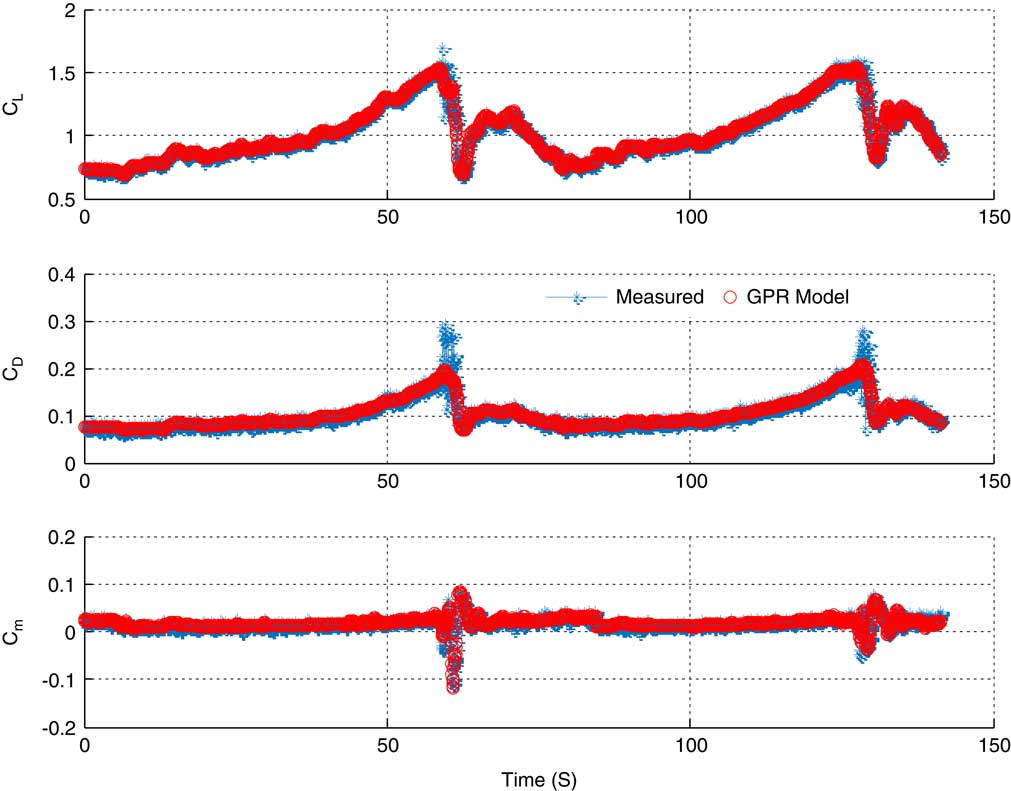
Figure 2 (Colour online) GPR model for lift force coefficient (C L), drag force coefficient (C D), and pitching moment coefficient (C m).
4.2 Non-linear modelling using MLE
Force and moment coefficients were also estimated with MLE using a parametric approach based on the quasi-steady model described in Eq. (9). MLE-estimated parameters were used in deriving aerodynamic forces and moments.
Estimated parameters using MLE are
 $$C_{{\rm D_{0} }} $$
=0.0435 [1.00]*, e=0.839 [0.82],
$$C_{{\rm D_{0} }} $$
=0.0435 [1.00]*, e=0.839 [0.82],
 $$C_{{\rm L_{0} }} $$
=0.158 [2.08],
$$C_{{\rm L_{0} }} $$
=0.158 [2.08],
 $$C_{{\rm L_{\ralpha } }} $$
=3.298 [1.14],
$$C_{{\rm L_{\ralpha } }} $$
=3.298 [1.14],
 $$C_{{\rm L_{{\ralpha M\ralpha }} }} $$
=9.07 [2.20],
$$C_{{\rm L_{{\ralpha M\ralpha }} }} $$
=9.07 [2.20],
 $$C_{{\rm m_{0} }} $$
=0.05 [3.50],
$$C_{{\rm m_{0} }} $$
=0.05 [3.50],
 $$C_{{\rm m_{\ralpha } }} $$
=−0.1763 [4.47],
$$C_{{\rm m_{\ralpha } }} $$
=−0.1763 [4.47],
 $$C_{{\rm m_{q} }} $$
=–6.146 [4.47],
$$C_{{\rm m_{q} }} $$
=–6.146 [4.47],
 $$C_{{\rm m_{{\delta e}} }} $$
=−0.391 [4.08], a
1=23.716 [3.41], α*=0.309 [0.35], τ2=24.025
$$C_{{\rm m_{{\delta e}} }} $$
=−0.391 [4.08], a
1=23.716 [3.41], α*=0.309 [0.35], τ2=24.025
 $${{\bar{c}} \over V}$$
[1.46],
$${{\bar{c}} \over V}$$
[1.46],
 $$C_{{\rm D_{X} }} $$
=0.0792 [3.82],
$$C_{{\rm D_{X} }} $$
=0.0792 [3.82],
 $$C_{{\rm m_{X} }} $$
= −0.1261 [3.98] with acceptable Cramer–Rao bounds. Number inside []* represent the relative standard deviation.
$$C_{{\rm m_{X} }} $$
= −0.1261 [3.98] with acceptable Cramer–Rao bounds. Number inside []* represent the relative standard deviation.
GPR Estimated C L, C D, and C m was compared with MLE estimated force and moment coefficients. Results are shown in Figs 3–9.
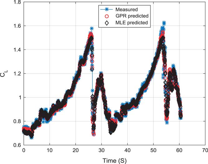
Figure 3 (Colour online) Validation of the lift force coefficient (C L).
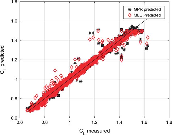
Figure 4 (Colour online) Prediction correlation of GPR estimated, and MLE estimated for lift force coefficient (C L).
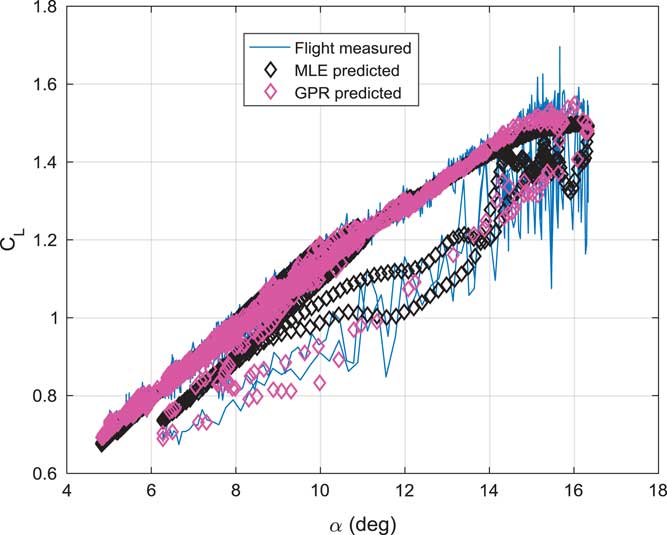
Figure 5 (Colour online) Stall hysteresis modelling.

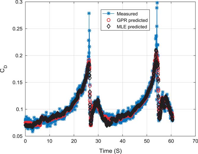
Figure 6 (Colour online) Validation of the drag force coefficient (C D).

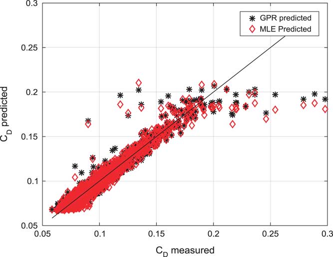
Figure 7 (Colour online) Measured and predicted drag force coefficient (C D).
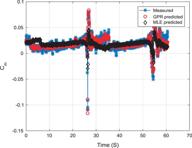
Figure 8 (Colour online) Validation of the pitching moment coefficient (C m).
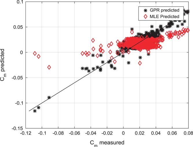
Figure 9 (Colour online) Measured and predicted pitching moment coefficient (C m).
Figure 3 shows the validation of the lift force coefficient (C L) using GPR and MLE. Estimated models were compared with a measured coefficient. All the curve are fitting on each other well. Estimated model using GPR are able to follow the MLE predicted and measured coefficient closely.
Figure 4 shows a prediction correlation study of GPR estimated and MLE estimated lift force coefficient (C L). GPR estimated lift force coefficient is following measured lift force coefficient.
Figure 5 shows the stall hysteresis modelling using C L and angle-of-attack data. GPR shows better prediction than MLE.
Figure 6 shows a validation of drag force coefficient (C D) using GPR and MLE. Estimated models were compared with a measured coefficient. All the curve are fitting on each other well. Estimated model using GPR are able to follow the MLE predicted and measured coefficient closely.
Figure 7 shows a prediction correlation study of GPR estimated and MLE estimated drag force coefficient (C D). GPR estimated lift force coefficient is following measured lift force coefficient.
Figure 8 shows the validation of pitching moment coefficient (C m) using GPR and MLE. Estimated models were compared with a measured coefficient. All the curve are fitting on each other well. Estimated model using GPR are able to follow the MLE predicted and measured coefficient closely.
Figure 9 shows a prediction correlation study of GPR estimated and MLE estimated pitching moment coefficient (C m). GPR estimated pitching moment coefficient are following measured pitching moment coefficient.
Table 1 presents the statistical comparison of estimated results. It shows prediction correlation for GPR and MLE. Prediction correlation for C L using GPR is found to be 0.9914 while 0.9898 is in MLE. Prediction correlation for C D using GPR is found to be 0.9545 while 0.9486 is in MLE. Prediction correlation for C m using GPR is found to be 0.9027 while 0.4669 is in MLE. There is a significant improvement in C m modelling using GPR approach. Statistical results show GPR can prove to be a compatible alternative for the application of non-linear force and moment coefficient modelling.
Table 1 Prediction correlation and RMSE calculation for MLE and GPR method

5.0 CONCLUSIONS
In this paper, the GPR-based novel method was proposed to estimate a non-linear aerodynamic model. The efficacy of the algorithm was examined on the DLR-ATTAS aircraft data. Non-linear model estimation was carried out using the Kernel-based probabilistic model in GPR. Further, the exponential squared function was chosen judiciously to use as a kernel function. GPR model was trained and validated with real flight data. Seventy per cent of the data were used in training, and the remaining 30% of the data were used for validation of the model.
Aerodynamic force and moment coefficients: Lift force coefficient (C L), drag force coefficient (C D), and pitching moment coefficient (C m) were estimated for ATTAS aircraft. Statistical modelling technique was used in quantifying the uncertainty in the model. GPR models were found to give mean errors of 2.7%, 0.8%, and 0.5% in coefficient of lift force, the coefficient of drag force, and coefficient of pitching moment, respectively. GPR estimated non-linear aerodynamic models were compared with MLE predicted models. MLE methods have been a popular classical method for several decades. Estimated results from both the methods were in close agreement with each other. GPR estimated model for C L and C D were reasonably close to MLE-estimated results. GPR-estimated C m were highly efficient in terms of correlation analysis. Presented results proved to make GPR as a promising alternative approach to this problem. GPR does not require to solve the equation of motion, this advantage further motivates promising directions for future research and can be readily generalised to other applications such as aeroelasticity, load estimation, and optimisation. Also, an extension of the GPR technique can be employed to boost the presented results.