NOMENCLATURE
- subscripts:
 $_{{3}/{4}}$
evaluated at
${3}/{4}$
chord point,
${}_{0}$
evaluated at
${\boldsymbol{p}}=0$
,
${}_{z}$
at unitary pitch,
${}_{c}$
at limit for unitary pitch
$_{{3}/{4}}$
evaluated at
${3}/{4}$
chord point,
${}_{0}$
evaluated at
${\boldsymbol{p}}=0$
,
${}_{z}$
at unitary pitch,
${}_{c}$
at limit for unitary pitchsuperscripts : ‘ time derivative of, “ second time derivative of
- c
chord of foil
- ec
-
$={\boldsymbol{F}}\hbox{-}{\boldsymbol{iG}} ={\boldsymbol{Re}}^{{\boldsymbol{-i}}\boldsymbol\theta}$
trail of quarter chord behind pitch axis
-
${\boldsymbol{g=G/k}}$
negative pitch damping rate of G
-
${\boldsymbol{h}}_{{\textbf{3}}/{\textbf{4}}}$
heave of pitch axis
- h ¾
heave of the
${3}/{4}$
chord point- i
square root of -1
- j
pitch inertia/
${}^{2}$
-
${\boldsymbol{k}} ={\boldsymbol{Ke}}^{{\boldsymbol{-i}}\boldsymbol\phi}$
reduced frequency based on chord
$\boldsymbol\omega{\boldsymbol{c/V}}$
-
${\boldsymbol{k}}_\textbf{n}$
reduced natural frequency
${\boldsymbol\omega}_{\textbf{n}}{\boldsymbol{c/V}}$
-
${\boldsymbol{k}}_{\textbf{c}}$
crtitical reduced natural frequency
- m
virtual mass of foil/unit length
- p
total mass/virtual
- q
distance of foil
${3}/{4}$
chord from axis in chords- r
non-d heave
- H
to pitch amplitude ratio
- t
time
- x
pitch imbalance/mc
- y
-
${\boldsymbol{e}} + {\mathbf{1}}/{\mathbf{4}}/{\boldsymbol{F}}$
- A
real effective non-dimensional inertia matrix about
${1}/{4}$
chord,
${\textbf{A}}_{1}$
complex,
${\textbf{A}}_{0}$
about pitch axis- B
non-dimensional aerodynamic damping matrix
- C
non-dimensional aerodynamic stiffness matrix
- E
non-dimensional elastic stiffness matrix
-
${\boldsymbol{E}}{}_{1}({\boldsymbol{u}})$
Exponential Integral function
${\boldsymbol{E}}_{1}({\boldsymbol{u}}) =\int^{\infty}_{1}\textbf{d}\boldsymbol{t}\textbf{e}^{-{\boldsymbol{ut}}}/{\boldsymbol{t}}$
- K
magnitude of complex k
- L
circulatory lift
- M
pitch stiffness torque/radian
- P
minimum p+1 due to stiffness effect of net fluid heave force
- N
nominal apparent wind at
${3}/{4}$
chord point angle
$\boldsymbol{\varphi}$
-
${\boldsymbol{O}}\, \textbf{=}\, {\boldsymbol{M}}/{\boldsymbol{mV}}^{\textbf{2}}$
pitch stiffness non-d. wrt nominal aerotorque
-
${\boldsymbol{\underline{Q}}}=(\textit{h}, {\boldsymbol \gamma})$
coordinate vector of heave and pitch displacements
- R
magnitude of T
- S
heave stiffness = heave spring force/h
-
${\boldsymbol{T}} ={\boldsymbol{F}}\hbox{-}{\boldsymbol{iG}} ={\boldsymbol{Re}}^{{\boldsymbol{-i}}\boldsymbol\theta}$
complex Theodorsen function of k
- U
upwash or normal component of the apparent wind N
- V
flowspeed
-
${\boldsymbol{Z}} ={\boldsymbol{M}}/ {\boldsymbol{Sc}}$
pitch vs heave stiffness
-
$\boldsymbol{\alpha}$
effective non-dimensional pitch inertia
-
$\boldsymbol{\beta}$
effective non-dimensional aero pitch damping
-
$\boldsymbol{\chi}$
effective non-dimensional aero pitch stiffness
-
${\boldsymbol \rho}$
Fluid density
-
${\boldsymbol \gamma}$
pitch angle
-
${\boldsymbol \gamma_{0}}$
pitch angle amplitude
-
${\boldsymbol \delta}\textbf{(}\boldsymbol{k}\textbf{)}$
discriminant of nil net aerodyanamic pitch damping
-
${\boldsymbol \phi}$
Polar angle of complex frequency k
-
${\boldsymbol \Gamma}$
complex amplitude of pitch
-
${\boldsymbol \gamma_{0}}$
amplitude of pitch (magnitude of
${\boldsymbol \Gamma}$
)-
${\boldsymbol \kappa}$
real (frequency) part of complex k
-
${\boldsymbol \lambda}$
minus the imaginary (growth) part of complex k
-
${\boldsymbol \theta}$
the negative of the Phase angle of Theodorsen Function
-
${\boldsymbol \varphi}$
$\,\,={\boldsymbol{F}}\hbox{-}{\boldsymbol{iG}} ={\boldsymbol{Re}}^{{\boldsymbol{-i}}\boldsymbol\theta}$
Nominal Angle-of-attack ignoring wake induction
-
${\boldsymbol \xi}$
phase lead of pitch ahead of heave (phase of
${\boldsymbol \Gamma}$
-
${\boldsymbol \omega}$
circular frequency in radians of phase/unit time
-
${\boldsymbol \omega}_{\mathrm{n}}$
natural frequency in heave
$\surd{{\boldsymbol{S}}}/\surd{{\boldsymbol{m}}}$


1.0 INTRODUCTION
Duncan(Reference Duncan1) recognised in the study of early aircraft flutter accidents that flutter’s spontaneous phased oscillations of the two ‘binary’ degrees of freedom were being powered by the airstream. He even built a heaving ‘engine’ that articulated a balanced foil to pitch and heave (or plunge) 90° out of phase to pedantically show this (and nothing more). In fact to safely tap the highly variable power of ambient flows requires exploiting the full two amplitude freedom of binary flutter(Reference Farthing2, Reference Farthing3). The FlutterWing’d Pump (FWP) originated in 1978 after the 1976 BBC broadcast of Pocklington School Young Scientists’ fluttering models promised better wind waterpumping than rotary multiblade windpumps, especially for developing countries. Prototypes have now pumped well and reliably for years but help is needed with commercialisation or adoption in the Third World.
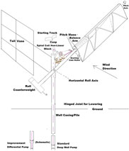
As in Fig. 1 the FWP has a wing free to pitch (360°) on top of a semi-rotary roll pendulum. In 1978 a model bore out our conjecture that its flutter could stop in a high wind to protect the FWP in storms. The non-linearities of large amplitude pitch and roll velocity greatly exceeding windspeed proved favourable experimentally without unduly compromising this high wind safety(Reference Farthing4). Extraordinary full-scale smoke video(Reference Farthing5) shows leading edge vortex shedding at full
 $\pm$
90° pitch flip. The pump connection itself has to be non-linear to limit the roll amplitude and absorb the variable windpower but not inhibit flutter starting. The Flutterwell base in Fig. 1 uses the steel well-casing as a foundation pile, whilst the Flo-Pump base floats around its pump cylinder and above its underwater outlet pipe to shore(Reference Farthing5).
$\pm$
90° pitch flip. The pump connection itself has to be non-linear to limit the roll amplitude and absorb the variable windpower but not inhibit flutter starting. The Flutterwell base in Fig. 1 uses the steel well-casing as a foundation pile, whilst the Flo-Pump base floats around its pump cylinder and above its underwater outlet pipe to shore(Reference Farthing5).
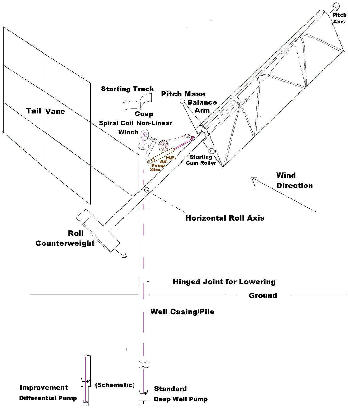
Figure 1. Schematic of the Flutterwell Pump, the well-mounted Flutter Wing Pump.
Underwater river or tidal current windmills have also been proposed but a counter-oscillating scale model with ferrocement blades failed to flutter. Approximate strip-theory flutter calculations were stable. A literature search could not find flutter in water. Ashley et al(Reference Ashley, Dugundji and Henry6) had presented experiments and computations showing an end to flutter as the mass ratio of typical blade weight distributions was lowered. So a quest began for a flutter design space in water and to understand flutter zones in a more general and analytical way for the basic heaving wing (mill) of chord c, virtual mass m, that is free to pivot about an axis ec leading the center of pressure(Reference Farthing3). The lack of pitch mechanical elasticity allowed (for the first time) flutter to be algebraically solved so the entire neutrally stable flutter space could be graphed and the influence of all parameters clearly understood. For instance, the reduced frequency
 ${\boldsymbol{k}}$
is independent of the heave stiffness or heave mass(Reference Farthing7) and only varies with net pitch inertia mc
${\boldsymbol{k}}$
is independent of the heave stiffness or heave mass(Reference Farthing7) and only varies with net pitch inertia mc
 ${}^{\mathbf{2}}$
j and mass imbalance mcx, as
${}^{\mathbf{2}}$
j and mass imbalance mcx, as
 \begin{equation}
{\mathbf{2}{\boldsymbol{ej}} + ({\boldsymbol{y}}-\mathbf{2}{\boldsymbol{eq}}){\boldsymbol{x}} - {\boldsymbol{qy}}} = {{1}}/{{2}}{{\boldsymbol{k}}^{2}(\,{\boldsymbol{j}} - {\boldsymbol{qx}})(\,{\boldsymbol{j}}-{\boldsymbol{yx}})/{\boldsymbol{F}}}
\label{eqn1}
\end{equation}
\begin{equation}
{\mathbf{2}{\boldsymbol{ej}} + ({\boldsymbol{y}}-\mathbf{2}{\boldsymbol{eq}}){\boldsymbol{x}} - {\boldsymbol{qy}}} = {{1}}/{{2}}{{\boldsymbol{k}}^{2}(\,{\boldsymbol{j}} - {\boldsymbol{qx}})(\,{\boldsymbol{j}}-{\boldsymbol{yx}})/{\boldsymbol{F}}}
\label{eqn1}
\end{equation}
where the pivot is
 ${\boldsymbol{q}}={\boldsymbol{e}}+\textbf{1/2}$
chords ahead of
${\boldsymbol{q}}={\boldsymbol{e}}+\textbf{1/2}$
chords ahead of
 ${3}/{4}$
chord,
${3}/{4}$
chord,
 ${\boldsymbol{y}}={\boldsymbol{e}} + \textbf{1/4/F,}$
and F(k) is the real part of the Theodorsen function (imaginary part -G ignored). The linear LHS and hyperbolic RHS vanish at the nexus
${\boldsymbol{y}}={\boldsymbol{e}} + \textbf{1/4/F,}$
and F(k) is the real part of the Theodorsen function (imaginary part -G ignored). The linear LHS and hyperbolic RHS vanish at the nexus
 $\boldsymbol{\mathcal{N}}=({\boldsymbol{q}}^{2}{\boldsymbol{,q}})$
of any k and the end post at
$\boldsymbol{\mathcal{N}}=({\boldsymbol{q}}^{2}{\boldsymbol{,q}})$
of any k and the end post at
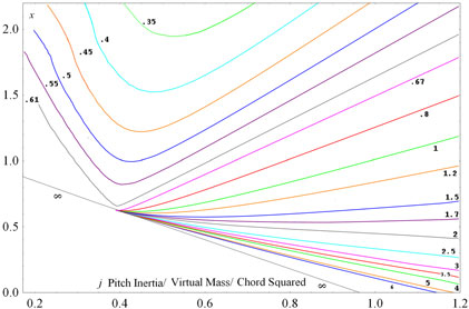
 ${\boldsymbol{j/Y}}={\boldsymbol{x}}=2{\boldsymbol{Y}}=\textbf{2e}+{1}/{2}\, \mathrm{of}\, {\boldsymbol{F}}=1 @ {\boldsymbol{k}}=0$
. Thus the k=0 quasisteady “qs” line between the nexus and endpost extends downwards in x with j so aerodynamic overbalance e with inertia j reduces the tailheaviness x for flutter, even to negative x noseheaviness.
${\boldsymbol{j/Y}}={\boldsymbol{x}}=2{\boldsymbol{Y}}=\textbf{2e}+{1}/{2}\, \mathrm{of}\, {\boldsymbol{F}}=1 @ {\boldsymbol{k}}=0$
. Thus the k=0 quasisteady “qs” line between the nexus and endpost extends downwards in x with j so aerodynamic overbalance e with inertia j reduces the tailheaviness x for flutter, even to negative x noseheaviness.
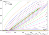
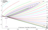
Numerically (1) was a soluble quadratic in x vs j along each contour value of k and F(k), allowing the entire contour space to be generated without iteration(Reference Farthing7). This opened up the final step to exactness in this paper of adding the small imaginary part -iG to F, with due consideration of the limiting behaviour of this poorly understood function G. Remarkably G only adds extra terms to the RHS of (1) and only in terms of G, and Gk which persists at high k to close the contours into ellipses that converge on the ray from the nexus
 $\mathcal{N}$
to 4
$\mathcal{N}$
to 4
 $\mathcal{N}$
. One concern was the effect of the G phase shift on P or the net stiffening of the fluid forces, undesirable with a stiffening pump. A greater was the singularity in G/k or its effective negative pitch damping at small k
$\mathcal{N}$
. One concern was the effect of the G phase shift on P or the net stiffening of the fluid forces, undesirable with a stiffening pump. A greater was the singularity in G/k or its effective negative pitch damping at small k
 $\downarrow$
0, which indeed will drastically change the small k contours at high inertia j, even allowing a pure pitch flutter.
$\downarrow$
0, which indeed will drastically change the small k contours at high inertia j, even allowing a pure pitch flutter.
2.0 COMPLEX THEODORSEN FUNCTION AND PURE PITCH FLUTTER
So as in Fig. 2, consider a unit length section of an infinite (vertical) symmetric airfoil of chord c, whose
 ${1}/{4}$
chord center of pressure point trails, by a distance ec, the pivot point of foil pitch at any angle
${1}/{4}$
chord center of pressure point trails, by a distance ec, the pivot point of foil pitch at any angle
 ${\gamma}$
to the stream velocity V. This trail
${\gamma}$
to the stream velocity V. This trail
 ${\boldsymbol{e}}\geq 0$
eliminates a divergence complicating typical wing bending-torsion flutter. For the fluttermill of Fig. 1, small
${\boldsymbol{e}}\geq 0$
eliminates a divergence complicating typical wing bending-torsion flutter. For the fluttermill of Fig. 1, small
 ${\boldsymbol{e}}\,\approx\,.03$
allows the bottom of the fabric-on-frame wing to pitch around an internal tubular steel spar cantilevered above the pendulum.
${\boldsymbol{e}}\,\approx\,.03$
allows the bottom of the fabric-on-frame wing to pitch around an internal tubular steel spar cantilevered above the pendulum.
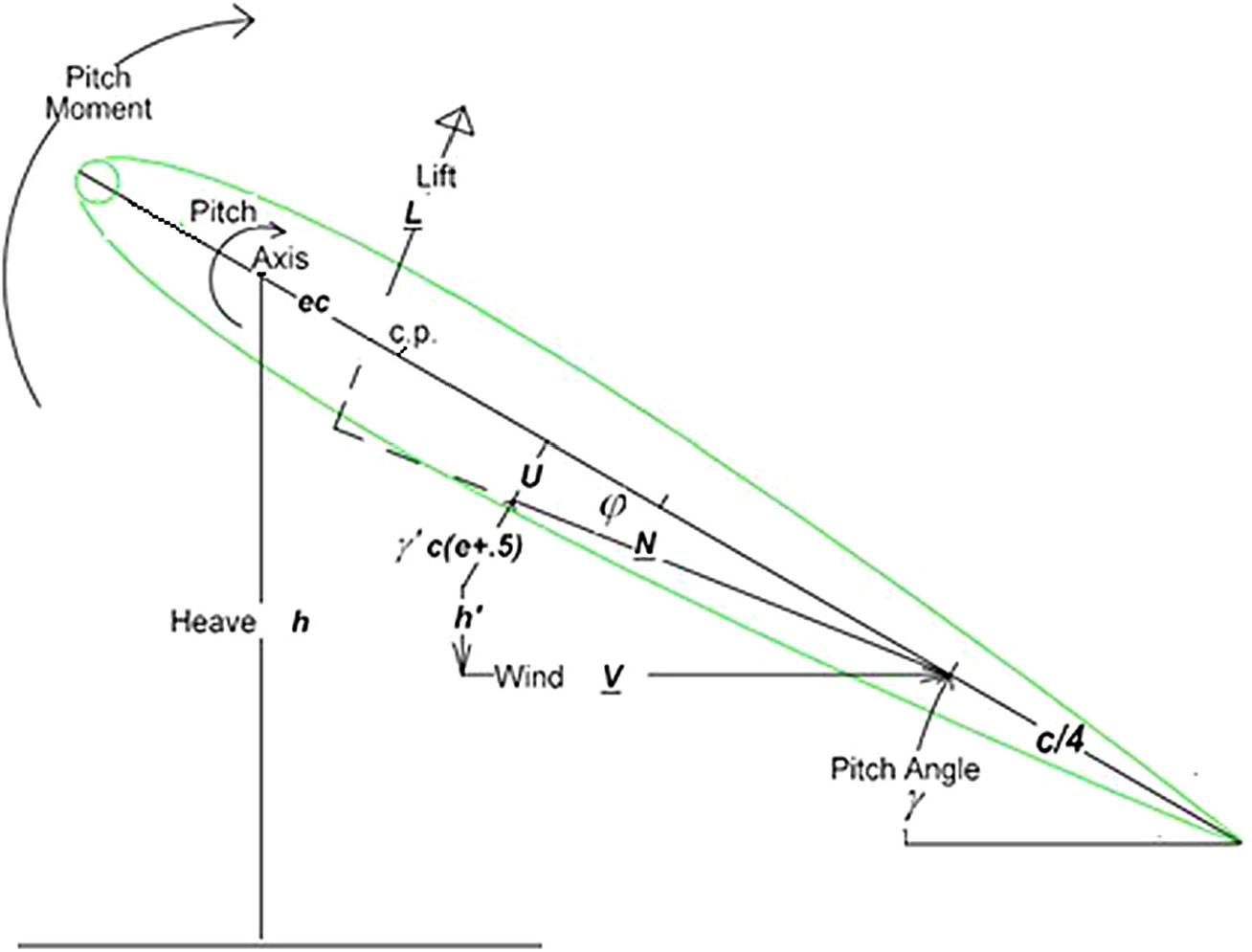
Figure 2. Section of Airfoil free in pitch and sprung in heave.
Pitch elastic stiffness would prevent FWP omnidirectionality to wind gusts(Reference Lighthill8) and would complicate bidirectionality in a tidal model. It is also absent in cantilevered ‘spade’ rudders on boats, if not on all-moving aircraft rudders and tails. But all such pitch axes may heave elastically cross-stream with coordinate h. For such thin airfoils, potential theory gives a virtual ‘added’ mass of
 ${\boldsymbol{m}} = {\textbf{1}}/{\textbf{4}}\boldsymbol\pi\rho{\boldsymbol{c}}^{2}$
as in the circumscribing cylinder of fluid of density
${\boldsymbol{m}} = {\textbf{1}}/{\textbf{4}}\boldsymbol\pi\rho{\boldsymbol{c}}^{2}$
as in the circumscribing cylinder of fluid of density
 ${\rho}$
centered at midchord. Use this simple m to define non-dimensional total
${\rho}$
centered at midchord. Use this simple m to define non-dimensional total
 $=$
virtual
$=$
virtual
 $+$
real mass, as pm for
$+$
real mass, as pm for
 ${\boldsymbol{p>}}1$
, total pitch axis (dynamic) imbalance as mxc and total inertia as
${\boldsymbol{p>}}1$
, total pitch axis (dynamic) imbalance as mxc and total inertia as
 ${\boldsymbol{mjc}}^{2}$
. The virtual intrinsic pitch inertia about midchord is
${\boldsymbol{mjc}}^{2}$
. The virtual intrinsic pitch inertia about midchord is
 ${\boldsymbol{mc}^{2}}/32$
, a factor of four less than a solid (i.e. ice) cylinder’s
${\boldsymbol{mc}^{2}}/32$
, a factor of four less than a solid (i.e. ice) cylinder’s
 ${\boldsymbol{mc}^{2}}/8$
. So the virtual inertia about
${\boldsymbol{mc}^{2}}/8$
. So the virtual inertia about
 ${1}/{4}$
chord center of pressure is
${1}/{4}$
chord center of pressure is
 $3{\boldsymbol{mc}^{2}}/32$
, half of a solid cylinder’s
$3{\boldsymbol{mc}^{2}}/32$
, half of a solid cylinder’s
 $3{\boldsymbol{mc}^{2}}/16$
and
$3{\boldsymbol{mc}^{2}}/16$
and
 ${3}/{8}$
of the nexal
${3}/{8}$
of the nexal
 ${\boldsymbol{q}^{2}}$
. Whilst the virtual imbalance is
${\boldsymbol{q}^{2}}$
. Whilst the virtual imbalance is
 ${1}/{2}$
of the nexal q, indeed insufficient for flutter which needs similar real imbalance, or several fold real inertia with
${1}/{2}$
of the nexal q, indeed insufficient for flutter which needs similar real imbalance, or several fold real inertia with
 ${\boldsymbol{e}}\gg 0$
(Reference Farthing7). Foil center of real structural mass is typically 35% c and certainly never ahead of
${\boldsymbol{e}}\gg 0$
(Reference Farthing7). Foil center of real structural mass is typically 35% c and certainly never ahead of
 ${1}/{4}$
chord and so increases x and j. The usual mass ratio is
${1}/{4}$
chord and so increases x and j. The usual mass ratio is
 ${\boldsymbol{p}}\hbox{-}1$
. Kinematically from real mass times real inertia
${\boldsymbol{p}}\hbox{-}1$
. Kinematically from real mass times real inertia
 $\geq$
real imbalance squared then
$\geq$
real imbalance squared then
 \begin{equation}
{\boldsymbol{p}}-1>({\boldsymbol{x}} - {\boldsymbol{e}} -{1}/{4})^{2} / (\,{\boldsymbol{j}}-({\boldsymbol{e}}+{1}/{4}){}^{2}-{1}/{32})
\label{eqn2}
\end{equation}
\begin{equation}
{\boldsymbol{p}}-1>({\boldsymbol{x}} - {\boldsymbol{e}} -{1}/{4})^{2} / (\,{\boldsymbol{j}}-({\boldsymbol{e}}+{1}/{4}){}^{2}-{1}/{32})
\label{eqn2}
\end{equation}
Fig. 2 shows the nominal apparent wind N at the
 ${3}/{4}$
chord point has angle-of-attack
${3}/{4}$
chord point has angle-of-attack
 \begin{equation}
\varphi=\gamma-{\textit{h}_{{3}/{4}}}^{'}/\textit{V}\ \ \mathrm{if}\ \textit{h}{}_{{3}/{4}}=\textit{h-cq}\gamma\ \ \varphi=\gamma-\textit{h}'\textit{V}+\textit{cq}\gamma `/\textit{V}
\label{eqn3}
\end{equation}
\begin{equation}
\varphi=\gamma-{\textit{h}_{{3}/{4}}}^{'}/\textit{V}\ \ \mathrm{if}\ \textit{h}{}_{{3}/{4}}=\textit{h-cq}\gamma\ \ \varphi=\gamma-\textit{h}'\textit{V}+\textit{cq}\gamma `/\textit{V}
\label{eqn3}
\end{equation}
With L the lift, the pitch moment balance per unit span about the pitch axis is
 \begin{equation}
{m}\{\gamma" {jc}^{2}+\gamma`{Vcq}-{h"xc}\} = -{ecL} = -{ec}\pi\rho{cV}^{2}{T}\varphi
\label{eqn4}
\end{equation}
\begin{equation}
{m}\{\gamma" {jc}^{2}+\gamma`{Vcq}-{h"xc}\} = -{ecL} = -{ec}\pi\rho{cV}^{2}{T}\varphi
\label{eqn4}
\end{equation}
Note the inertial { } in (4) is
 ${\boldsymbol{Vqc}}{\boldsymbol{\varphi}}'$
at the nexus
${\boldsymbol{Vqc}}{\boldsymbol{\varphi}}'$
at the nexus
 $\boldsymbol{\mathcal{N}}$
 ${\boldsymbol{j}}= {\boldsymbol{xq}}$
and
${\boldsymbol{j}}= {\boldsymbol{xq}}$
and
 ${\boldsymbol{x}} ={\boldsymbol{q}}$
where feathering
${\boldsymbol{x}} ={\boldsymbol{q}}$
where feathering
 $\boldsymbol{\varphi}= 0$
thus balances pitch. A virtual mass m at the
$\boldsymbol{\varphi}= 0$
thus balances pitch. A virtual mass m at the
 ${3}/{4}$
chord point has such
${3}/{4}$
chord point has such
 ${\boldsymbol{j}} $
and
${\boldsymbol{j}} $
and
 ${\boldsymbol{x.}}$
The unsteady lift L is based on the addition of wake-induced flow to N to form the true apparent wind W at true angle-of-attack
 ${\boldsymbol{T}}{\boldsymbol\varphi}$
for small amplitude oscillation of frequency
${\boldsymbol{T}}{\boldsymbol\varphi}$
for small amplitude oscillation of frequency
 $\boldsymbol{\omega}$
. So
$\boldsymbol{\omega}$
. So
 ${\boldsymbol{L}}={\boldsymbol{\pi\rho}}{\boldsymbol{cV}}^{2}{\boldsymbol{T}}{\boldsymbol\varphi}=\boldsymbol{4mVTU/c}$
where
${\boldsymbol{L}}={\boldsymbol{\pi\rho}}{\boldsymbol{cV}}^{2}{\boldsymbol{T}}{\boldsymbol\varphi}=\boldsymbol{4mVTU/c}$
where
 ${\boldsymbol{U}}={\boldsymbol{V}}{\boldsymbol\varphi}= {\boldsymbol{V}}{\boldsymbol\gamma} -{\boldsymbol{h}}'+{\boldsymbol{cq}}{\boldsymbol\gamma}`$
is the nominal normal flow at
${\boldsymbol{U}}={\boldsymbol{V}}{\boldsymbol\varphi}= {\boldsymbol{V}}{\boldsymbol\gamma} -{\boldsymbol{h}}'+{\boldsymbol{cq}}{\boldsymbol\gamma}`$
is the nominal normal flow at
 ${3}/{4}$
chord and
${3}/{4}$
chord and
 $\boldsymbol\pi{{\boldsymbol{cU}}}$
is the nominal circulation.
$\boldsymbol\pi{{\boldsymbol{cU}}}$
is the nominal circulation.
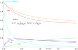
 ${\boldsymbol{T}(\textit{k) =F-iG}}$
graphed in Fig. 3 is the complex Theodorsen wake function of reduced frequency
${\boldsymbol{T}(\textit{k) =F-iG}}$
graphed in Fig. 3 is the complex Theodorsen wake function of reduced frequency
 ${\boldsymbol{k}}={\boldsymbol{\omega}}{\boldsymbol{c/V.}}$
Where K
 ${}_{n}$
are modified Bessel functions of the second kind
${}_{n}$
are modified Bessel functions of the second kind
 \begin{equation}
\textit{T}(\textit{k)=F-iG=K}_{1}({1}/{2}\textit{ik})/\{\textit{K}_{0}({1}/{2}\textit{ik})+\textit{K}_{1}({1}/{2}\textit{ik})\}=1/ (1+\textit{K}_{0}({1}/{2}\textit{ik})\textit{/K}_{1}({1}/{2}\textit{ik}))
\label{eqn5}
\end{equation}
\begin{equation}
\textit{T}(\textit{k)=F-iG=K}_{1}({1}/{2}\textit{ik})/\{\textit{K}_{0}({1}/{2}\textit{ik})+\textit{K}_{1}({1}/{2}\textit{ik})\}=1/ (1+\textit{K}_{0}({1}/{2}\textit{ik})\textit{/K}_{1}({1}/{2}\textit{ik}))
\label{eqn5}
\end{equation}
9.7.2(Reference Abramowitz and Stegun9) gives asymptotes as
 ${\boldsymbol{K}}_{\textbf{0}}/ {\boldsymbol{K}}_{\textbf{1}} = 1 - {1}/{2}/{\boldsymbol{z}} +\ldots = 1 + {\boldsymbol{i}}/{\boldsymbol{k}} +\ldots$
so
${\boldsymbol{K}}_{\textbf{0}}/ {\boldsymbol{K}}_{\textbf{1}} = 1 - {1}/{2}/{\boldsymbol{z}} +\ldots = 1 + {\boldsymbol{i}}/{\boldsymbol{k}} +\ldots$
so
 ${\boldsymbol{F}}={1}/{2}\, (+ {1}/{4}/ {\boldsymbol{k}}^2+\cdot\cdot)$
and
${\boldsymbol{F}}={1}/{2}\, (+ {1}/{4}/ {\boldsymbol{k}}^2+\cdot\cdot)$
and
 ${\boldsymbol{G}} = {1}/{4} /{\boldsymbol{k}}\, (-7/ 16{\boldsymbol{k}}^{3}+\cdot\cdot)$
. Note the slow decay of G as 1/k, slower than
${\boldsymbol{G}} = {1}/{4} /{\boldsymbol{k}}\, (-7/ 16{\boldsymbol{k}}^{3}+\cdot\cdot)$
. Note the slow decay of G as 1/k, slower than
 ${\boldsymbol{F}}$
 $\uparrow$
 $\textbf{{1}/{2}}$
as 1/
$\textbf{{1}/{2}}$
as 1/
 ${\boldsymbol{k}}^{{\boldsymbol{2}}}$
, which will affect the character of the binary stability contours at large k.
${\boldsymbol{k}}^{{\boldsymbol{2}}}$
, which will affect the character of the binary stability contours at large k.

Figure 3. F Real and G Negative Imaginary parts of T(k) and of its approximation.
The actual circulation
 ${\boldsymbol \pi}{\boldsymbol{cVT}}{\boldsymbol \varphi}$
time change with complex extended implicit
${\boldsymbol \pi}{\boldsymbol{cVT}}{\boldsymbol \varphi}$
time change with complex extended implicit
 $\textbf{e}^{{\boldsymbol{i}} \boldsymbol \omega {\boldsymbol{t}}}$
is shed into the wake vortex sheet at linear density
$\textbf{e}^{{\boldsymbol{i}} \boldsymbol \omega {\boldsymbol{t}}}$
is shed into the wake vortex sheet at linear density
 $\Lambda = {\boldsymbol{i}}{\boldsymbol\omega\pi} {\boldsymbol{cT}}\boldsymbol\varphi \textbf{e}^{-{\boldsymbol{i}} \boldsymbol \omega {\boldsymbol{x/v}}}$
at
$\Lambda = {\boldsymbol{i}}{\boldsymbol\omega\pi} {\boldsymbol{cT}}\boldsymbol\varphi \textbf{e}^{-{\boldsymbol{i}} \boldsymbol \omega {\boldsymbol{x/v}}}$
at
 ${\boldsymbol{x}} = {\boldsymbol{zc}}$
behind the trailing edge, back-inducing a midchord angle attack
${\boldsymbol{x}} = {\boldsymbol{zc}}$
behind the trailing edge, back-inducing a midchord angle attack
 $\Lambda \text{d}{\boldsymbol{x}}/2\pi {\boldsymbol{V}}({\boldsymbol{x}}+\textbf{{1}/{2}}{\boldsymbol{c}})$
. Integrating the influence
$\Lambda \text{d}{\boldsymbol{x}}/2\pi {\boldsymbol{V}}({\boldsymbol{x}}+\textbf{{1}/{2}}{\boldsymbol{c}})$
. Integrating the influence
 $\boldsymbol{I}=\int_0^\infty {\boldsymbol{ik}}\ \textbf{{e}}^{-{\boldsymbol{ikz}}}\text{d}{\boldsymbol{z}}/ 2({\boldsymbol{z}} + {1}/{2}) \approx\,(1-\boldsymbol{T})/\boldsymbol{T}$
so
$\boldsymbol{I}=\int_0^\infty {\boldsymbol{ik}}\ \textbf{{e}}^{-{\boldsymbol{ikz}}}\text{d}{\boldsymbol{z}}/ 2({\boldsymbol{z}} + {1}/{2}) \approx\,(1-\boldsymbol{T})/\boldsymbol{T}$
so
 $\boldsymbol{F}-\boldsymbol{iG}$
behaves as
$\boldsymbol{F}-\boldsymbol{iG}$
behaves as
 ${\boldsymbol{T}} \approx 1/\ 1+{\boldsymbol{I}}$
. Though the exact
${\boldsymbol{T}} \approx 1/\ 1+{\boldsymbol{I}}$
. Though the exact
 ${\boldsymbol{T}}$
and the circulation distribution inside the foil micro-satisfy no net crossflow at any point within the thin foil.
${\boldsymbol{T}}$
and the circulation distribution inside the foil micro-satisfy no net crossflow at any point within the thin foil.
 ${\boldsymbol{G}}$
has a little-recognised singularity in its slope and negative implicit damping
${\boldsymbol{G}}$
has a little-recognised singularity in its slope and negative implicit damping
 ${\boldsymbol{g}}={\boldsymbol{G}}/{\boldsymbol{k}}={\boldsymbol{dG/dk}} {\uparrow}-\textbf{{1}/{2}}\textbf{Ln}(\textbf{{1}/{2}}{\boldsymbol{k}})$
as
${\boldsymbol{g}}={\boldsymbol{G}}/{\boldsymbol{k}}={\boldsymbol{dG/dk}} {\uparrow}-\textbf{{1}/{2}}\textbf{Ln}(\textbf{{1}/{2}}{\boldsymbol{k}})$
as
 ${\boldsymbol{k}}\downarrow0:\, {\boldsymbol{T}}\rightarrow\textbf{1}-{\boldsymbol{K}}_{0}(\textbf{{1}/{2}}{\boldsymbol{ik}})/{\boldsymbol{K}}_{1}(\textbf{{1}/{2}}{\boldsymbol{ik}})$
9.6.8(Reference Abramowitz and Stegun9) gives
${\boldsymbol{k}}\downarrow0:\, {\boldsymbol{T}}\rightarrow\textbf{1}-{\boldsymbol{K}}_{0}(\textbf{{1}/{2}}{\boldsymbol{ik}})/{\boldsymbol{K}}_{1}(\textbf{{1}/{2}}{\boldsymbol{ik}})$
9.6.8(Reference Abramowitz and Stegun9) gives
 ${\boldsymbol{K}}_{0}(\textbf{{1}/{2}}{\boldsymbol{ik}}) {\downarrow}-{\boldsymbol{Ln}}(\textbf{{1}/{2}}{\boldsymbol{ik}})$
and 9.6.9(Reference Abramowitz and Stegun9)
${\boldsymbol{K}}_{0}(\textbf{{1}/{2}}{\boldsymbol{ik}}) {\downarrow}-{\boldsymbol{Ln}}(\textbf{{1}/{2}}{\boldsymbol{ik}})$
and 9.6.9(Reference Abramowitz and Stegun9)
 ${\boldsymbol{K}}_{1}(\textbf{{1}/{2}}{\boldsymbol{ik}})=\textbf{2}/{\boldsymbol{ik.}}$
So as
${\boldsymbol{K}}_{1}(\textbf{{1}/{2}}{\boldsymbol{ik}})=\textbf{2}/{\boldsymbol{ik.}}$
So as
 $\textit{k}\downarrow 0,$
 \begin{equation}
\textit{T}\rightarrow 1+{1}/{2}\textit{ik}(\text{Ln}({1}/{2}\textit{k})+{1}/{2}\textit{i}\pi),\ \textit{F}\rightarrow 1-{1}/{4}\pi\textit{k}\ \text{and}\ {g=G/k}{\uparrow}-{1}/{2}\text{Ln}({1}/{2}\textit{k})
\label{eqn6}
\end{equation}
\begin{equation}
\textit{T}\rightarrow 1+{1}/{2}\textit{ik}(\text{Ln}({1}/{2}\textit{k})+{1}/{2}\textit{i}\pi),\ \textit{F}\rightarrow 1-{1}/{4}\pi\textit{k}\ \text{and}\ {g=G/k}{\uparrow}-{1}/{2}\text{Ln}({1}/{2}\textit{k})
\label{eqn6}
\end{equation}
Responsible for G’s negative pitch damping is the dominant vorticity shed out of phase at the trailing edge, inducing negative apparent wind at the foil reducing the lift at the c.p. for a positive pitch-increasing moment correction about the axis
 ${\boldsymbol{ec}}$
further ahead. The shed strength is as
${\boldsymbol{ec}}$
further ahead. The shed strength is as
 ${\boldsymbol{k}}$
and its effective extent is many
${\boldsymbol{k}}$
and its effective extent is many
 $\textbf{{1}/{2}}{\boldsymbol \pi}/{\boldsymbol{k}}$
chords, so (for an
$\textbf{{1}/{2}}{\boldsymbol \pi}/{\boldsymbol{k}}$
chords, so (for an
 ${\boldsymbol{AR}} {\boldsymbol\rightarrow \infty}$
wing with an even greater span) truncating
${\boldsymbol{AR}} {\boldsymbol\rightarrow \infty}$
wing with an even greater span) truncating
 ${\boldsymbol{I}}$
there gives
${\boldsymbol{I}}$
there gives
 $\boldsymbol{k}\downarrow 0,\,\boldsymbol{G}$
as
$\boldsymbol{k}\downarrow 0,\,\boldsymbol{G}$
as
 $-{1}/{2}{\boldsymbol{ik}}\textbf{Ln}({\boldsymbol{k}}).$
Midchord is where Wagner’s
$-{1}/{2}{\boldsymbol{ik}}\textbf{Ln}({\boldsymbol{k}}).$
Midchord is where Wagner’s
 ${1}/{2}$
vortex shed at the t.e. counter-induces half of a sudden angle
${1}/{2}$
vortex shed at the t.e. counter-induces half of a sudden angle
 $\gamma$
, so evaluate
$\gamma$
, so evaluate
 ${\boldsymbol{I}}=\int^{\infty}_{0}{\boldsymbol{ik}}\textbf{e}^{-\boldsymbol{ikz}} \text{d}{\boldsymbol{z/}} 2({\boldsymbol{z}}+{1}/{2})$
at midchord. If
${\boldsymbol{I}}=\int^{\infty}_{0}{\boldsymbol{ik}}\textbf{e}^{-\boldsymbol{ikz}} \text{d}{\boldsymbol{z/}} 2({\boldsymbol{z}}+{1}/{2})$
at midchord. If
 $\textit{u}=2{\boldsymbol{z}}+1,\,{\boldsymbol{I}}= {1}/{2}{\boldsymbol{ik}}\textbf{e}^{\textbf{{1}/{2}}\boldsymbol{ik}} \int^{\infty}_{1}d{\boldsymbol{u}}\, \textbf{e-}^{\textbf{{1}/{2}}\boldsymbol{iku}}/{\boldsymbol{u}}={\boldsymbol{v}}\textbf{e}^{{\boldsymbol{v}}}\boldsymbol{E}_{1}(\boldsymbol{v})$
if
$\textit{u}=2{\boldsymbol{z}}+1,\,{\boldsymbol{I}}= {1}/{2}{\boldsymbol{ik}}\textbf{e}^{\textbf{{1}/{2}}\boldsymbol{ik}} \int^{\infty}_{1}d{\boldsymbol{u}}\, \textbf{e-}^{\textbf{{1}/{2}}\boldsymbol{iku}}/{\boldsymbol{u}}={\boldsymbol{v}}\textbf{e}^{{\boldsymbol{v}}}\boldsymbol{E}_{1}(\boldsymbol{v})$
if
 ${\boldsymbol{v}}=\textbf{1/2}{\boldsymbol{ik}}$
, as in Fig. 3. Integrating this revised
${\boldsymbol{v}}=\textbf{1/2}{\boldsymbol{ik}}$
, as in Fig. 3. Integrating this revised
 ${\boldsymbol{I}}$
twice by parts gives
${\boldsymbol{I}}$
twice by parts gives
 ${\boldsymbol{I}}\rightarrow 1+O({\boldsymbol{i}}/ {\boldsymbol{k}})$
for the correct limit
${\boldsymbol{I}}\rightarrow 1+O({\boldsymbol{i}}/ {\boldsymbol{k}})$
for the correct limit
 ${\boldsymbol{T}}\downarrow{1}/{2}$
at large
${\boldsymbol{T}}\downarrow{1}/{2}$
at large
 ${\boldsymbol{k}}$
. The maximum in
${\boldsymbol{k}}$
. The maximum in
 ${\boldsymbol{G}}$
is due to the increase in shed vortex strength as
${\boldsymbol{G}}$
is due to the increase in shed vortex strength as
 ${\boldsymbol{k}}$
being countered by the closing of previously oppositely shed in
${\boldsymbol{k}}$
being countered by the closing of previously oppositely shed in
 ${\boldsymbol{I}}$
.
${\boldsymbol{I}}$
.
Note that the
 ${\boldsymbol{T}}$
solution holds for a decaying far wake in unstable growth(Reference Jones10) i.e.
${\boldsymbol{T}}$
solution holds for a decaying far wake in unstable growth(Reference Jones10) i.e.
 ${\boldsymbol{k}}={\boldsymbol{K}}e^{-i\phi} = \boldsymbol\kappa-{\boldsymbol{i}}{\lambda}$
as contoured in Fig. 4. Wake attenuation drops the peak
${\boldsymbol{k}}={\boldsymbol{K}}e^{-i\phi} = \boldsymbol\kappa-{\boldsymbol{i}}{\lambda}$
as contoured in Fig. 4. Wake attenuation drops the peak
 $\boldsymbol{G}$
and shifts it to higher
$\boldsymbol{G}$
and shifts it to higher
 ${\boldsymbol{k}}$
. The
${\boldsymbol{k}}$
. The
 ${\boldsymbol{F}}$
contours are near circles in .
${\boldsymbol{F}}$
contours are near circles in .
 $1\lt{\boldsymbol{K}}\lt{1}/{2}$
, as at first the general wake attenuation is offset by the greater dominance of the
$1\lt{\boldsymbol{K}}\lt{1}/{2}$
, as at first the general wake attenuation is offset by the greater dominance of the
 $\textbf{{1}/{2}}\boldsymbol\pi/{\boldsymbol{k}}$
peak over
$\textbf{{1}/{2}}\boldsymbol\pi/{\boldsymbol{k}}$
peak over
 ${3}/{2}{\boldsymbol \pi}/{\boldsymbol{k}}$
reversal in
${3}/{2}{\boldsymbol \pi}/{\boldsymbol{k}}$
reversal in
 ${\boldsymbol{I}}$
, etc. But for
${\boldsymbol{I}}$
, etc. But for
 ${\boldsymbol{K}}>\textbf{1/2}$
the offset of the trailing edge shed point from the midchord induction point causes the attenuation to dominate and increase
${\boldsymbol{K}}>\textbf{1/2}$
the offset of the trailing edge shed point from the midchord induction point causes the attenuation to dominate and increase
 ${\boldsymbol{F}}$
with
${\boldsymbol{F}}$
with
 $\boldsymbol{\lambda}$
. The real T for divergence
$\boldsymbol{\lambda}$
. The real T for divergence
 $\kappa = 0$
decreases with
$\kappa = 0$
decreases with
 $\lambda$
from one to asymptote to the Wagner
$\lambda$
from one to asymptote to the Wagner
 ${1}/{2}$
.
${1}/{2}$
.

Figure 4. Plot of complex Theodorsen function in 4
 ${}^{\mathrm{th}}$
quadrant of complex plane.
${}^{\mathrm{th}}$
quadrant of complex plane.
Extend
 ${\boldsymbol{h/c}}$
to the complex domain as
${\boldsymbol{h/c}}$
to the complex domain as
 $\textbf{e}^{\boldsymbol{i}{\boldsymbol \omega}\boldsymbol{t}}{\boldsymbol{H}}$
and likewise
$\textbf{e}^{\boldsymbol{i}{\boldsymbol \omega}\boldsymbol{t}}{\boldsymbol{H}}$
and likewise
 ${\boldsymbol\gamma}=\textbf{e}^{{\boldsymbol{i}{\boldsymbol \omega}\boldsymbol{t}}}{\boldsymbol\Gamma}$
where
${\boldsymbol\gamma}=\textbf{e}^{{\boldsymbol{i}{\boldsymbol \omega}\boldsymbol{t}}}{\boldsymbol\Gamma}$
where
 ${\boldsymbol \Gamma}={\boldsymbol\gamma}_{0}\textbf{e}^{\boldsymbol{i}\xi}$
where
${\boldsymbol \Gamma}={\boldsymbol\gamma}_{0}\textbf{e}^{\boldsymbol{i}\xi}$
where
 ${\boldsymbol\gamma}_{\textbf{0}}$
is the amplitude of
${\boldsymbol\gamma}_{\textbf{0}}$
is the amplitude of
 $\gamma$
and
$\gamma$
and
 $\xi$
its phase lead over real
$\xi$
its phase lead over real
 ${\boldsymbol{H}}$
.
${\boldsymbol{H}}$
.
 ${\boldsymbol{L}}$
complex extends to
${\boldsymbol{L}}$
complex extends to
 \begin{equation}
\textit{L}= \pi\rho cV^{2}T\{\Gamma-ikH+ikq\Gamma \}\mathrm{e}^{\mathrm{i}\omega t}
\label{eqn7}
\end{equation}
\begin{equation}
\textit{L}= \pi\rho cV^{2}T\{\Gamma-ikH+ikq\Gamma \}\mathrm{e}^{\mathrm{i}\omega t}
\label{eqn7}
\end{equation}
Dividing (4) by
 $\textit{mV}^{2}$
 $\text{e}^{\mathrm{i}\omega t}$
 \begin{equation}
\Gamma \{-k^{2}j+ikq(1+4eT)+4eT\}+H\{k^{2}x-4ikeT\}=0
\label{eqn8}
\end{equation}
\begin{equation}
\Gamma \{-k^{2}j+ikq(1+4eT)+4eT\}+H\{k^{2}x-4ikeT\}=0
\label{eqn8}
\end{equation}
so with
 ${\boldsymbol{H}}=0$
,
${\boldsymbol{H}}=0$
,
 ${\boldsymbol{K}}={\boldsymbol{K}}\text{e}^{-\boldsymbol\iota\phi} \ \boldsymbol{T}=\boldsymbol{R}\text{e}^{-\boldsymbol{\iota\theta}}$
multiply by e
${\boldsymbol{K}}={\boldsymbol{K}}\text{e}^{-\boldsymbol\iota\phi} \ \boldsymbol{T}=\boldsymbol{R}\text{e}^{-\boldsymbol{\iota\theta}}$
multiply by e
 $^{2\boldsymbol\iota\phi}$
for
$^{2\boldsymbol\iota\phi}$
for
 $\boldsymbol{K}^{2}\boldsymbol{j}=\boldsymbol{ik}\text{e}^{\boldsymbol\iota\phi}\boldsymbol{q}(\textbf{1}+\boldsymbol{4eT})+\boldsymbol{4eT}\text{e}^{2\iota\phi}$
so the real part
$\boldsymbol{K}^{2}\boldsymbol{j}=\boldsymbol{ik}\text{e}^{\boldsymbol\iota\phi}\boldsymbol{q}(\textbf{1}+\boldsymbol{4eT})+\boldsymbol{4eT}\text{e}^{2\iota\phi}$
so the real part
 \begin{equation}
\textit{K}^{2}\textit{j}=-\textit{Kq}(\sin\phi+4eR\sin(\phi-\theta))+4eR\cos(2\phi-\theta)
\label{eqn9}
\end{equation}
\begin{equation}
\textit{K}^{2}\textit{j}=-\textit{Kq}(\sin\phi+4eR\sin(\phi-\theta))+4eR\cos(2\phi-\theta)
\label{eqn9}
\end{equation}
isolates
 ${\boldsymbol{j}},$
leaving the imaginary part:
${\boldsymbol{j}},$
leaving the imaginary part:
 $K(e+{1}/{2})(\cos\phi+4eR{\cos}(\phi-\theta))+ 4eR{\sin}(2\phi-\theta)=0$
or the quadratic
$K(e+{1}/{2})(\cos\phi+4eR{\cos}(\phi-\theta))+ 4eR{\sin}(2\phi-\theta)=0$
or the quadratic
 \begin{align}
4e^{2}RK{\cos}(\phi-\theta)+e\{K{\cos}\phi+2KR{\cos}(\phi-\theta)+4R{\sin}(2\phi-\theta)\}+{1}/{2}K{\cos}\phi=0
\label{eqn10}
\end{align}
\begin{align}
4e^{2}RK{\cos}(\phi-\theta)+e\{K{\cos}\phi+2KR{\cos}(\phi-\theta)+4R{\sin}(2\phi-\theta)\}+{1}/{2}K{\cos}\phi=0
\label{eqn10}
\end{align}
whose solution
 ${\boldsymbol{e}}$
and corresponding
${\boldsymbol{e}}$
and corresponding
 ${\boldsymbol{j}}$
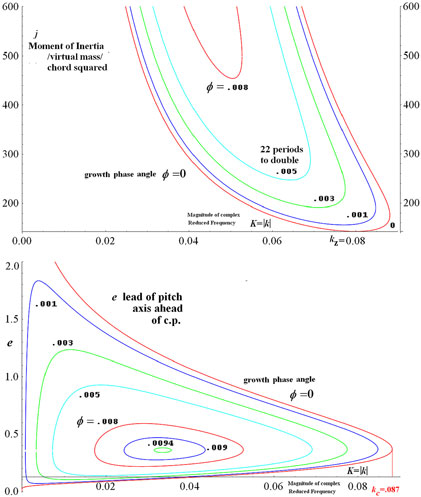
is graphed in Fig. 5 versus
${\boldsymbol{j}}$
is graphed in Fig. 5 versus
 ${\boldsymbol{K}}$
with
${\boldsymbol{K}}$
with
 $\boldsymbol{\phi}$
as a parameter. At
$\boldsymbol{\phi}$
as a parameter. At
 ${\boldsymbol{\phi}}=.008$
(vs maximum
${\boldsymbol{\phi}}=.008$
(vs maximum
 $\boldsymbol{\phi}=.095$
) the minimum
$\boldsymbol{\phi}=.095$
) the minimum
 ${\boldsymbol{j}}$
is 455 and the periods-to-double is Ln2/
${\boldsymbol{j}}$
is 455 and the periods-to-double is Ln2/
 $.0016\pi \,\approx\, 14$
not fast enough as a windmill to respond to wind changes. As the pitch amplitude
$.0016\pi \,\approx\, 14$
not fast enough as a windmill to respond to wind changes. As the pitch amplitude
 ${\boldsymbol\gamma}_{0}$
increases, the foil would readily stall at this low
${\boldsymbol\gamma}_{0}$
increases, the foil would readily stall at this low
 ${\boldsymbol{k}}$
without any heave apparent wind and significant swept area, so the power per foil area would remain poor.
${\boldsymbol{k}}$
without any heave apparent wind and significant swept area, so the power per foil area would remain poor.
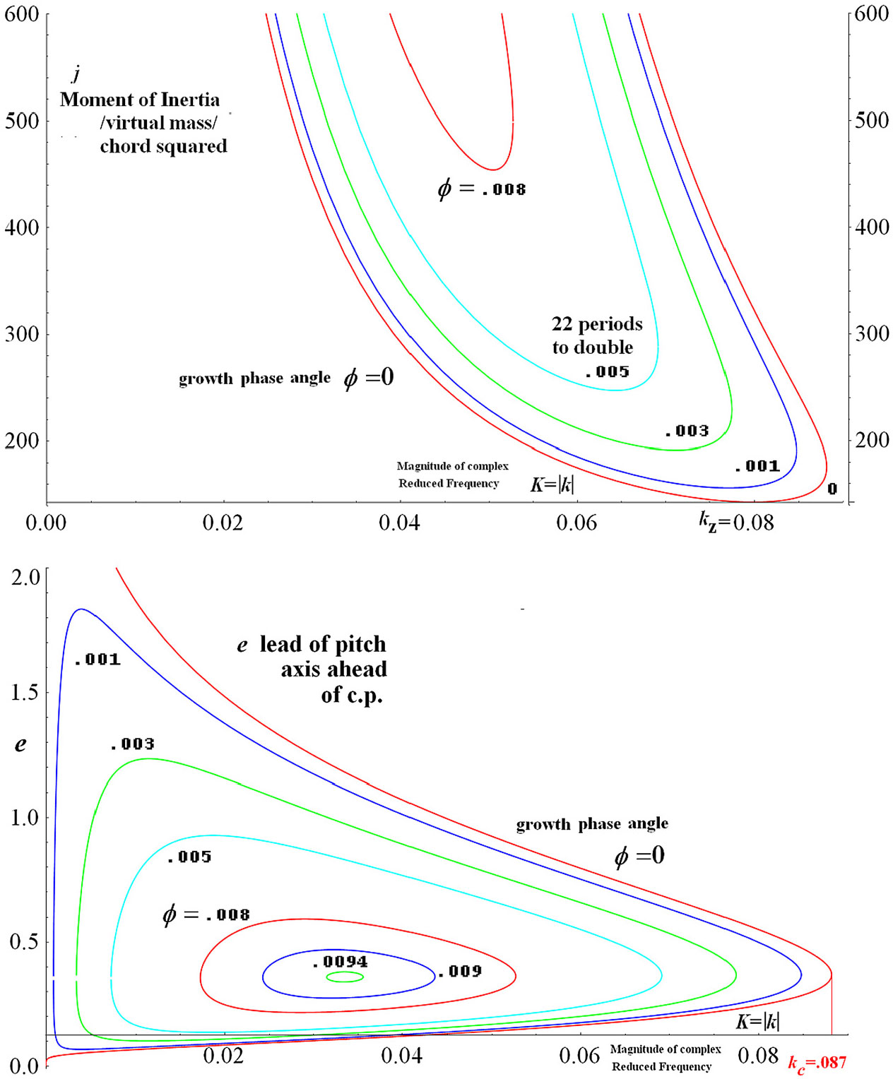
Figure 5. e and j contours of pure pitch flutter vs reduced frequency at different growth phase.
Now consider neutral stability
 ${\boldsymbol \phi}=0$
with its minimum
${\boldsymbol \phi}=0$
with its minimum
 ${\boldsymbol{j}}$
of 143 at
${\boldsymbol{j}}$
of 143 at
 $\boldsymbol{k}_{\boldsymbol{z}}(\boldsymbol{e})=.0798$
at
$\boldsymbol{k}_{\boldsymbol{z}}(\boldsymbol{e})=.0798$
at
 ${\boldsymbol{e}} =.244$
. Shifting the
${\boldsymbol{e}} =.244$
. Shifting the
 ${\boldsymbol{gk}}$
’s in
${\boldsymbol{gk}}$
’s in
 ${\boldsymbol{T}}={\boldsymbol{F}}-{\boldsymbol{ikg}}$
for real coefficients, and with
${\boldsymbol{T}}={\boldsymbol{F}}-{\boldsymbol{ikg}}$
for real coefficients, and with
 ${\boldsymbol{Fy}}={\boldsymbol{Fe}}+{1}/{4}$
and real
${\boldsymbol{Fy}}={\boldsymbol{Fe}}+{1}/{4}$
and real
 ${\boldsymbol{\alpha}} =\boldsymbol{j}-\mathbf{4}\boldsymbol{qge}$
,
${\boldsymbol{\alpha}} =\boldsymbol{j}-\mathbf{4}\boldsymbol{qge}$
,
 ${\boldsymbol{\beta}}=\mathbf{4}\boldsymbol{qyF}-\mathbf{4}\boldsymbol{eg}$
,
${\boldsymbol{\beta}}=\mathbf{4}\boldsymbol{qyF}-\mathbf{4}\boldsymbol{eg}$
,
 $\boldsymbol{\chi}=\mathbf{4}\boldsymbol{eF}$
reduces (8) to
$\boldsymbol{\chi}=\mathbf{4}\boldsymbol{eF}$
reduces (8) to
 \begin{equation}
\Gamma[-k^{2}\alpha+ik\beta+\chi]+H[k^{2}(x-4eg)-4ikeF]=0
\label{eqn11}
\end{equation}
\begin{equation}
\Gamma[-k^{2}\alpha+ik\beta+\chi]+H[k^{2}(x-4eg)-4ikeF]=0
\label{eqn11}
\end{equation}
Non zero pitch-only –
 ${\boldsymbol{k}}^{2}{\boldsymbol{\alpha}}+\boldsymbol{ik}{\boldsymbol{\beta}}+\boldsymbol{\chi} =0$
oscillation persists when
${\boldsymbol{k}}^{2}{\boldsymbol{\alpha}}+\boldsymbol{ik}{\boldsymbol{\beta}}+\boldsymbol{\chi} =0$
oscillation persists when
 ${\boldsymbol{\beta}}=0={\boldsymbol{qyF}}-{\boldsymbol{eg}}$
requiring simplified (10):
${\boldsymbol{\beta}}=0={\boldsymbol{qyF}}-{\boldsymbol{eg}}$
requiring simplified (10):
 $\boldsymbol{4e}^{2}\boldsymbol{F}-\textbf{(}\boldsymbol{4g}-\boldsymbol{2F}-\textbf{1}\textbf{)}\boldsymbol{e}+\textbf{1/2}={\bf 0}$
(10b). Note the real roots merge and end at the (first) zero of the discriminant
$\boldsymbol{4e}^{2}\boldsymbol{F}-\textbf{(}\boldsymbol{4g}-\boldsymbol{2F}-\textbf{1}\textbf{)}\boldsymbol{e}+\textbf{1/2}={\bf 0}$
(10b). Note the real roots merge and end at the (first) zero of the discriminant
 $\delta = \textbf{(4}\boldsymbol{g}-\textbf{2}\boldsymbol{F}-\textbf{1)}^{\textbf{2}}-8\boldsymbol{F}$
or dividing by four,
$\delta = \textbf{(4}\boldsymbol{g}-\textbf{2}\boldsymbol{F}-\textbf{1)}^{\textbf{2}}-8\boldsymbol{F}$
or dividing by four,
 \begin{equation}
{1}/{4}\delta=(2g-F-{1}/{2})^{2}-2F=0
\label{eqn12}
\end{equation}
\begin{equation}
{1}/{4}\delta=(2g-F-{1}/{2})^{2}-2F=0
\label{eqn12}
\end{equation}
solved by
 $\boldsymbol{2g}=\boldsymbol{F}+\textbf{1/2}+\surd{2}{\boldsymbol{F}}$
, with
$\boldsymbol{2g}=\boldsymbol{F}+\textbf{1/2}+\surd{2}{\boldsymbol{F}}$
, with
 ${\boldsymbol{F}}\,\approx\,1$
,
${\boldsymbol{F}}\,\approx\,1$
,
 ${\boldsymbol{g}}_{c}\,\approx\, {3}/{4} +\surd{1}/{2}=1.46$
.
${\boldsymbol{g}}_{c}\,\approx\, {3}/{4} +\surd{1}/{2}=1.46$
.
 ${\boldsymbol{F}}\,\approx\,.95$
refines to
${\boldsymbol{F}}\,\approx\,.95$
refines to
 ${\boldsymbol{g}}_{c}=1.41$
at
${\boldsymbol{g}}_{c}=1.41$
at
 ${\boldsymbol{k}}_{c}=.087$
. Now
${\boldsymbol{k}}_{c}=.087$
. Now
 $\boldsymbol{\chi}=\boldsymbol{k}^{\textbf{2}}{\boldsymbol{\alpha}}$
or
$\boldsymbol{\chi}=\boldsymbol{k}^{\textbf{2}}{\boldsymbol{\alpha}}$
or
 $\boldsymbol{4eF}= \boldsymbol{k}^{\textbf{2}}\textbf{(}\,\boldsymbol{j}-\boldsymbol{4qge)}=\boldsymbol{k}^{\textbf{2}}(\,\boldsymbol{j}-\textbf{4}\boldsymbol{q}^{\textbf{2}}\boldsymbol{yF})\cong\boldsymbol{k}^{\textbf{2}}\boldsymbol{j}$
(9b), so small e and small k combine to require a very large j. The unstable zone is between the e roots and between their corresponding. j’s. Let the subscript
$\boldsymbol{4eF}= \boldsymbol{k}^{\textbf{2}}\textbf{(}\,\boldsymbol{j}-\boldsymbol{4qge)}=\boldsymbol{k}^{\textbf{2}}(\,\boldsymbol{j}-\textbf{4}\boldsymbol{q}^{\textbf{2}}\boldsymbol{yF})\cong\boldsymbol{k}^{\textbf{2}}\boldsymbol{j}$
(9b), so small e and small k combine to require a very large j. The unstable zone is between the e roots and between their corresponding. j’s. Let the subscript
 ${}_{z}$
denote the more likely lower root. When the roots are very different this smaller has
${}_{z}$
denote the more likely lower root. When the roots are very different this smaller has
 ${\boldsymbol{g}}_{\boldsymbol{z}}= \textbf{3/4} +{1}/{\,8}\boldsymbol{e}$
. Elastic stiffness torque
${\boldsymbol{g}}_{\boldsymbol{z}}= \textbf{3/4} +{1}/{\,8}\boldsymbol{e}$
. Elastic stiffness torque
 ${\boldsymbol{M}}={\boldsymbol{OmV}}^{\textbf{2}}$
per radian would just add to
${\boldsymbol{M}}={\boldsymbol{OmV}}^{\textbf{2}}$
per radian would just add to
 ${\boldsymbol{j}}$
as
${\boldsymbol{j}}$
as
 $\boldsymbol\Delta\boldsymbol{j}=\boldsymbol{O}/{\boldsymbol{k}}_{\boldsymbol{z}}^{\textbf{2}}$
and distort
$\boldsymbol\Delta\boldsymbol{j}=\boldsymbol{O}/{\boldsymbol{k}}_{\boldsymbol{z}}^{\textbf{2}}$
and distort
 ${\boldsymbol \phi}=0$
upwards in the upper Fig. 5.
${\boldsymbol \phi}=0$
upwards in the upper Fig. 5.
Now consider the heave forces due to pitch:
 ${\boldsymbol{m}}\{{\boldsymbol\gamma}^{\prime}{\boldsymbol{V}}+{\boldsymbol\gamma} ^{\prime\prime}{\boldsymbol{xc}}\} + {\boldsymbol{L}}$
or in complex extension
${\boldsymbol{m}}\{{\boldsymbol\gamma}^{\prime}{\boldsymbol{V}}+{\boldsymbol\gamma} ^{\prime\prime}{\boldsymbol{xc}}\} + {\boldsymbol{L}}$
or in complex extension
 $\boldsymbol{mV}^{\textbf{2}}\textbf{e}^{\boldsymbol{i}\boldsymbol\omega \boldsymbol{t}}/\boldsymbol{c}$
times
$\boldsymbol{mV}^{\textbf{2}}\textbf{e}^{\boldsymbol{i}\boldsymbol\omega \boldsymbol{t}}/\boldsymbol{c}$
times
 ${\boldsymbol{ik}}{\boldsymbol\Gamma}-\boldsymbol{k}^{\textbf{2}}\boldsymbol\Gamma\boldsymbol{x}+\textbf{4(}\boldsymbol{F}-\boldsymbol{iG}\textbf{)} \{\boldsymbol\Gamma+{\boldsymbol{ikq}}{\boldsymbol \Gamma}\}$
. For no net heave force from pitch and so no heave motion, the coefficient of
${\boldsymbol{ik}}{\boldsymbol\Gamma}-\boldsymbol{k}^{\textbf{2}}\boldsymbol\Gamma\boldsymbol{x}+\textbf{4(}\boldsymbol{F}-\boldsymbol{iG}\textbf{)} \{\boldsymbol\Gamma+{\boldsymbol{ikq}}{\boldsymbol \Gamma}\}$
. For no net heave force from pitch and so no heave motion, the coefficient of
 ${\boldsymbol \Gamma}$
must vanish. Its imaginary quadrature part is
${\boldsymbol \Gamma}$
must vanish. Its imaginary quadrature part is
 $4{\boldsymbol{ik}}\textbf{(}\textbf{{1}/{4}}+{\boldsymbol{Fq}}-\boldsymbol{g}\textbf{)}=0$
. But
$4{\boldsymbol{ik}}\textbf{(}\textbf{{1}/{4}}+{\boldsymbol{Fq}}-\boldsymbol{g}\textbf{)}=0$
. But
 ${\boldsymbol{\beta}}={\boldsymbol{Fqy}}-{\boldsymbol{eg}}=0$
gives
${\boldsymbol{\beta}}={\boldsymbol{Fqy}}-{\boldsymbol{eg}}=0$
gives
 $\textbf{{1}/{4}}+{\boldsymbol{Fq}}-{\boldsymbol{g}}=-{1}/{8}/{\boldsymbol{e}}$
so
$\textbf{{1}/{4}}+{\boldsymbol{Fq}}-{\boldsymbol{g}}=-{1}/{8}/{\boldsymbol{e}}$
so
 $-{1}/{2}{\boldsymbol{ik}}{\boldsymbol \Gamma}{\boldsymbol{/e}}$
is the non-d. heave force in quadrature behind pitch. So a binary mode of pure pitch and perfectly free but quiescent heave cannot be balanced at any finite
$-{1}/{2}{\boldsymbol{ik}}{\boldsymbol \Gamma}{\boldsymbol{/e}}$
is the non-d. heave force in quadrature behind pitch. So a binary mode of pure pitch and perfectly free but quiescent heave cannot be balanced at any finite
 ${\boldsymbol{e}}.$
The above unitary mode implies heave immobilised by infinite stiffness of the pitch axis in heave.
${\boldsymbol{e}}.$
The above unitary mode implies heave immobilised by infinite stiffness of the pitch axis in heave.
3.0 BINARY PITCH AND HEAVE FLUTTER
So now allow heave h by relaxing the spring restoring force to a finite S per unit heave.
 \begin{equation}
{\boldsymbol{Sh}}+{\boldsymbol{m}}({\boldsymbol{p}}-1){\boldsymbol{h}}^{\prime\prime}={\boldsymbol{m}}\{-{\boldsymbol{h}}^{\prime\prime}+\gamma^{\prime}{\boldsymbol{V}}+\gamma^{\prime\prime} {\boldsymbol{xc}}\}+{\boldsymbol{L}}={\boldsymbol{Pmh}}^{\prime\prime}
\label{eqn13}
\end{equation}
\begin{equation}
{\boldsymbol{Sh}}+{\boldsymbol{m}}({\boldsymbol{p}}-1){\boldsymbol{h}}^{\prime\prime}={\boldsymbol{m}}\{-{\boldsymbol{h}}^{\prime\prime}+\gamma^{\prime}{\boldsymbol{V}}+\gamma^{\prime\prime} {\boldsymbol{xc}}\}+{\boldsymbol{L}}={\boldsymbol{Pmh}}^{\prime\prime}
\label{eqn13}
\end{equation}
The virtual/cross inertia {} bracket is
 ${\boldsymbol{V}}{\boldsymbol \varphi}'$
at the nexal
${\boldsymbol{V}}{\boldsymbol \varphi}'$
at the nexal
 ${\boldsymbol{x}}={\boldsymbol{q}}$
, so there (with
${\boldsymbol{x}}={\boldsymbol{q}}$
, so there (with
 $\boldsymbol\omega^{2}={\boldsymbol{S}}/ {\boldsymbol{m}}\textbf{(}\,{\boldsymbol{p}}-\textbf{1)}$
the no-fluid natural frequency),
$\boldsymbol\omega^{2}={\boldsymbol{S}}/ {\boldsymbol{m}}\textbf{(}\,{\boldsymbol{p}}-\textbf{1)}$
the no-fluid natural frequency),
 ${\boldsymbol \varphi}={\boldsymbol{L}}=0$
solves (4) and (13) at any
${\boldsymbol \varphi}={\boldsymbol{L}}=0$
solves (4) and (13) at any
 ${\boldsymbol{T}}$
and
${\boldsymbol{T}}$
and
 ${\boldsymbol{V}}$
and so for all
${\boldsymbol{V}}$
and so for all
 ${\boldsymbol{k}}={\boldsymbol\omega}{\boldsymbol{c/V}}$
. Thus flutter contours of all complex k including all growth contours go through the nexus
${\boldsymbol{k}}={\boldsymbol\omega}{\boldsymbol{c/V}}$
. Thus flutter contours of all complex k including all growth contours go through the nexus
 $\boldsymbol{\mathcal{N}}$
. Also a sinusoidal solution h of
$\boldsymbol{\mathcal{N}}$
. Also a sinusoidal solution h of
 $\boldsymbol\omega$
need not change when the heave mass p and stiffness S are changed in harmony as
$\boldsymbol\omega$
need not change when the heave mass p and stiffness S are changed in harmony as
 $\Delta{\boldsymbol{S}}={\boldsymbol{m}}\omega^{2}\Delta{\boldsymbol{p}}$
. So a solution at one p solves at any other with only S changed. That means solving
$\Delta{\boldsymbol{S}}={\boldsymbol{m}}\omega^{2}\Delta{\boldsymbol{p}}$
. So a solution at one p solves at any other with only S changed. That means solving
 ${\boldsymbol{H}}/{\boldsymbol \Gamma}$
and k will not depend upon p, so it can be made at
${\boldsymbol{H}}/{\boldsymbol \Gamma}$
and k will not depend upon p, so it can be made at
 ${\boldsymbol{p}}=0$
for great convenience and simplicity. Exactly the same intuition applies to the free-in-pitch 3D semi-rotary windmill that the roll inertia and stiffness will not enter the k equation. But this separation
${\boldsymbol{p}}=0$
for great convenience and simplicity. Exactly the same intuition applies to the free-in-pitch 3D semi-rotary windmill that the roll inertia and stiffness will not enter the k equation. But this separation
 $\Delta{\boldsymbol{S}}={\boldsymbol{m}}{\boldsymbol \omega}^{2} \Delta{\boldsymbol{p}}$
(and likewise
$\Delta{\boldsymbol{S}}={\boldsymbol{m}}{\boldsymbol \omega}^{2} \Delta{\boldsymbol{p}}$
(and likewise
 ${\boldsymbol \Delta}{\boldsymbol{j}}={\boldsymbol{Ok}}^{-2})$
fails for growth i.e. complex
${\boldsymbol \Delta}{\boldsymbol{j}}={\boldsymbol{Ok}}^{-2})$
fails for growth i.e. complex
 ${\boldsymbol \omega}^{2}$
and
${\boldsymbol \omega}^{2}$
and
 ${\boldsymbol{K}}^{2}$
. Eqn. (13) calls Pmh
${\boldsymbol{K}}^{2}$
. Eqn. (13) calls Pmh
 $^{\prime\prime}$
the net sinusoidal real mass inertia less the spring force equal to the middle net fluid & imbalance heave force. In
$^{\prime\prime}$
the net sinusoidal real mass inertia less the spring force equal to the middle net fluid & imbalance heave force. In
 ${\boldsymbol{G}}=0 $
flutter(Reference Farthing7)
${\boldsymbol{G}}=0 $
flutter(Reference Farthing7)
 ${\boldsymbol{P}} \lt 0$
at
${\boldsymbol{P}} \lt 0$
at
 ${\boldsymbol{k}} = 0$
beyond the nexus but grows positive with k as
${\boldsymbol{k}} = 0$
beyond the nexus but grows positive with k as
 ${\boldsymbol \varphi} \approx \gamma-{\boldsymbol{h}}^{\prime}/{\boldsymbol{V}}$
drives
${\boldsymbol \varphi} \approx \gamma-{\boldsymbol{h}}^{\prime}/{\boldsymbol{V}}$
drives
 ${\boldsymbol{h}}^{\prime}$
so
${\boldsymbol{h}}^{\prime}$
so
 ${\boldsymbol\varphi}^{\prime}\approx \gamma^{\prime}-{\boldsymbol{h}}^{\prime\prime}/{\boldsymbol{V}}$
phases with
${\boldsymbol\varphi}^{\prime}\approx \gamma^{\prime}-{\boldsymbol{h}}^{\prime\prime}/{\boldsymbol{V}}$
phases with
 $+{\boldsymbol{h}}^{\prime\prime}$
for net virtual mass and middle term stiffening. If
$+{\boldsymbol{h}}^{\prime\prime}$
for net virtual mass and middle term stiffening. If
 $\boldsymbol\omega_{\textbf{n}}$
is the natural frequency of just the virtual mass under S, and its reduced real
$\boldsymbol\omega_{\textbf{n}}$
is the natural frequency of just the virtual mass under S, and its reduced real
 ${\boldsymbol{k}}_{\textbf{n}} = {\boldsymbol \omega}_{\textbf{n}}{\boldsymbol{c/V}}$
, then
${\boldsymbol{k}}_{\textbf{n}} = {\boldsymbol \omega}_{\textbf{n}}{\boldsymbol{c/V}}$
, then
 \begin{equation}
\textit{S}=\textit{m}{\boldsymbol \omega}_{\mathrm{n}}^{2}=(\textit{p}-\textit{P}-1)\textit{m}\omega^{2}\ \text{so}\ \textit{k}_{\mathrm{n}}^{2}=(\textit{p}-\textit{P}-1)\textit{k}^{2}\ \mathrm{needs}\ \textit{p}>P+1
\label{eqn14}
\end{equation}
\begin{equation}
\textit{S}=\textit{m}{\boldsymbol \omega}_{\mathrm{n}}^{2}=(\textit{p}-\textit{P}-1)\textit{m}\omega^{2}\ \text{so}\ \textit{k}_{\mathrm{n}}^{2}=(\textit{p}-\textit{P}-1)\textit{k}^{2}\ \mathrm{needs}\ \textit{p}>P+1
\label{eqn14}
\end{equation}
From (13)
 ${\boldsymbol{m}}{\boldsymbol \omega}_{\textbf{n}}^{2}{\boldsymbol{h}}={\boldsymbol{m}}\{-{\boldsymbol{ph}}^{\prime\prime}+\boldsymbol\gamma' {\boldsymbol{V}} + \boldsymbol\gamma^{\prime\prime}{\boldsymbol{xc}}\}+{\boldsymbol{L}}$
so complex extending and dividing by
${\boldsymbol{m}}{\boldsymbol \omega}_{\textbf{n}}^{2}{\boldsymbol{h}}={\boldsymbol{m}}\{-{\boldsymbol{ph}}^{\prime\prime}+\boldsymbol\gamma' {\boldsymbol{V}} + \boldsymbol\gamma^{\prime\prime}{\boldsymbol{xc}}\}+{\boldsymbol{L}}$
so complex extending and dividing by
 $mV^{2}\text{e}^{i\omega t}/c$
,
$mV^{2}\text{e}^{i\omega t}/c$
,
 \begin{equation}
\Gamma\{k^{2}x-ik(1+4Tq)-4T\}+H\{k^{2}_{\mathrm{n}}-pk^{2}+4ikT\}=0
\label{eqn15}
\end{equation}
\begin{equation}
\Gamma\{k^{2}x-ik(1+4Tq)-4T\}+H\{k^{2}_{\mathrm{n}}-pk^{2}+4ikT\}=0
\label{eqn15}
\end{equation}
Let Q be the vector of coordinates
 $(\boldsymbol\Gamma, {\boldsymbol{H}})$
. A ‘derivative’ matrix form of the small amplitude equations of neutral stability oscillation (8) and (15) is
$(\boldsymbol\Gamma, {\boldsymbol{H}})$
. A ‘derivative’ matrix form of the small amplitude equations of neutral stability oscillation (8) and (15) is
 $(–{\boldsymbol{k}}^{2}\underline{\text{A}}_0+{\boldsymbol{ik}}\underline{\text{B}}_0+\underline{\text{C}}_0+{\boldsymbol{k}}_{\mathrm{n}}^2 \underline{\text{E}}_{0}) \textbf{Q}\,=\,0$
 \begin{gather}
\underline{\text{A}}_{0}=\left(\begin{array}{cc}
\boldsymbol{j} & {\rm -}{\boldsymbol{x}} \\
{\rm -}{\boldsymbol{x}} & {\boldsymbol{p}} \end{array}\right)\quad \underline{\text{B}}_{0}=\left( \begin{array}{cc}
\boldsymbol{q}{\rm +}{\mathbf 4}{{\boldsymbol{qTe}}} & {\rm -}{\mathbf 4}{{\boldsymbol{eT}}} \\
{\rm -}{\rm 1}{\rm -}{\mathbf 4}{{\boldsymbol{Tq}}} & {\mathbf 4}{{\boldsymbol{T}}} \end{array}
\right)\quad \underline{\text{C}}_{0}=\left( \begin{array}{cc}
{\mathbf 4}{{\boldsymbol{eT}}} & 0 \\
{\rm -}{\mathbf 4}{{\boldsymbol{T}}} & 0 \end{array}
\right)\quad \underline{\text{E}}_{0}=\left( \begin{array}{cc}
0 & 0 \\
0 & 1 \end{array}
\right)
\label{eqn16}
\end{gather}
\begin{gather}
\underline{\text{A}}_{0}=\left(\begin{array}{cc}
\boldsymbol{j} & {\rm -}{\boldsymbol{x}} \\
{\rm -}{\boldsymbol{x}} & {\boldsymbol{p}} \end{array}\right)\quad \underline{\text{B}}_{0}=\left( \begin{array}{cc}
\boldsymbol{q}{\rm +}{\mathbf 4}{{\boldsymbol{qTe}}} & {\rm -}{\mathbf 4}{{\boldsymbol{eT}}} \\
{\rm -}{\rm 1}{\rm -}{\mathbf 4}{{\boldsymbol{Tq}}} & {\mathbf 4}{{\boldsymbol{T}}} \end{array}
\right)\quad \underline{\text{C}}_{0}=\left( \begin{array}{cc}
{\mathbf 4}{{\boldsymbol{eT}}} & 0 \\
{\rm -}{\mathbf 4}{{\boldsymbol{T}}} & 0 \end{array}
\right)\quad \underline{\text{E}}_{0}=\left( \begin{array}{cc}
0 & 0 \\
0 & 1 \end{array}
\right)
\label{eqn16}
\end{gather}
Expanding
 ${\boldsymbol{T}}={\boldsymbol{F}}-{\boldsymbol{igk}}$
will allow shifting the gk terms leftwards to the next matrix to make them all real to get. (
${\boldsymbol{T}}={\boldsymbol{F}}-{\boldsymbol{igk}}$
will allow shifting the gk terms leftwards to the next matrix to make them all real to get. (
 $-\boldsymbol{k}^{2} \underbar{\text{A}}+{\boldsymbol{ik}}\underbar{\text{B}}+\underbar{\text{C}}+ {\boldsymbol{k}}_{\mathrm{n}}^{2} \underbar{\text{E}}$
)
$-\boldsymbol{k}^{2} \underbar{\text{A}}+{\boldsymbol{ik}}\underbar{\text{B}}+\underbar{\text{C}}+ {\boldsymbol{k}}_{\mathrm{n}}^{2} \underbar{\text{E}}$
)
 $\textbf{Q}={\underbar{\textbf{M}}\textbf{Q}}=0$
.
$\textbf{Q}={\underbar{\textbf{M}}\textbf{Q}}=0$
.
The cross determinant notation
 $[\textbf{J,K}]=\text{J}_{11}\text{K}_{22}+\text{J}_{22}\text{K}_{11}-\text{J}_{12}\text{K}_{21}-\text{J}_{21}\text{K}_{12}$
expands the nil determinant of this real matrix
$[\textbf{J,K}]=\text{J}_{11}\text{K}_{22}+\text{J}_{22}\text{K}_{11}-\text{J}_{12}\text{K}_{21}-\text{J}_{21}\text{K}_{12}$
expands the nil determinant of this real matrix
 $|\underline{\textbf{M}}| =0$
for neutral oscillatory stability in powers of k as
$|\underline{\textbf{M}}| =0$
for neutral oscillatory stability in powers of k as
 \begin{align}
&k^{4}|\underline{\text{A}}| -ik^{3}[\underline{\text{A}},\underline{\text{B}}] -k^{2}\!\left(|\underline{\text{B}}|+[\underline{\text{A}},\underline{\text{C}}]+[\underline{\text{A}},\underline{\text{E}}]k_{\mathrm{n}}^2\right) +ik\!\left(\hbox{\sout{[{\underline{\text{B}}},{\underline{\text{C}}}]}}+[\underline{\text{B}},\underline{\text{E}}]k_{\mathrm{n}}^2\right)\nonumber\\ & \qquad\qquad\qquad\qquad\qquad\qquad\qquad\quad\quad \ \ +\left(\hbox{\sout{|{\underline{\text{C}}}|}}+[\underline{\text{C}},\underline{\text{E}}]k_{\mathrm{n}}^2+\hbox{\sout{|{\underline{\text{E}}}|}}k_{\mathrm{n}}^4\right)=0
\label{eqn17}\end{align}
\begin{align}
&k^{4}|\underline{\text{A}}| -ik^{3}[\underline{\text{A}},\underline{\text{B}}] -k^{2}\!\left(|\underline{\text{B}}|+[\underline{\text{A}},\underline{\text{C}}]+[\underline{\text{A}},\underline{\text{E}}]k_{\mathrm{n}}^2\right) +ik\!\left(\hbox{\sout{[{\underline{\text{B}}},{\underline{\text{C}}}]}}+[\underline{\text{B}},\underline{\text{E}}]k_{\mathrm{n}}^2\right)\nonumber\\ & \qquad\qquad\qquad\qquad\qquad\qquad\qquad\quad\quad \ \ +\left(\hbox{\sout{|{\underline{\text{C}}}|}}+[\underline{\text{C}},\underline{\text{E}}]k_{\mathrm{n}}^2+\hbox{\sout{|{\underline{\text{E}}}|}}k_{\mathrm{n}}^4\right)=0
\label{eqn17}\end{align}
where the three crossed-outerms will vanish here. Then Re and Im of (17)
 \begin{align}
&|\underline{\text{A}}|k^4- \left(|\underline{\text{B}}|+[\underline{\text{A}},\underline{\text{C}}]+\alpha k_{\mathrm{n}}^2\right)k^2+\chi k_{\mathrm{n}}^2=0\label{eqn18}\end{align}
\begin{align}
&|\underline{\text{A}}|k^4- \left(|\underline{\text{B}}|+[\underline{\text{A}},\underline{\text{C}}]+\alpha k_{\mathrm{n}}^2\right)k^2+\chi k_{\mathrm{n}}^2=0\label{eqn18}\end{align}
 \begin{align} &\qquad\qquad[\underline{\text{A}},\underline{\text{B}}]k^2=\beta k_{\mathrm{n}}^2
\label{eqn19}\end{align}
\begin{align} &\qquad\qquad[\underline{\text{A}},\underline{\text{B}}]k^2=\beta k_{\mathrm{n}}^2
\label{eqn19}\end{align}
As the one
 ${\textit{E}}_0$
stiffness gives (after the gk shift to real matrices) pitch-only values from above
${\textit{E}}_0$
stiffness gives (after the gk shift to real matrices) pitch-only values from above
 \begin{equation}
[\underline{\text{A}},\underline{\text{E}}]=\alpha=\textit{j}-4\textit{qge}, [\underline{\text{B}},\underline{\text{E}}]=\beta=4\textit{qyF}-4\textit{eg}, [\underline{\text{C}},\underline{\text{E}}]=\chi=4\textit{eF}
\label{eqn20}
\end{equation}
\begin{equation}
[\underline{\text{A}},\underline{\text{E}}]=\alpha=\textit{j}-4\textit{qge}, [\underline{\text{B}},\underline{\text{E}}]=\beta=4\textit{qyF}-4\textit{eg}, [\underline{\text{C}},\underline{\text{E}}]=\chi=4\textit{eF}
\label{eqn20}
\end{equation}
To obtain the non-E binary real determinants, first form the moment equation about the c.p without the complex T by adding to (8) ec times the heave equation (15) (second row to the first in (15)) to get sparser B
 ${}_{1}$
and C
${}_{1}$
and C
 ${}_{1}$
 \begin{align}
\underline{\text{A}}_{\textbf{1}}=\left(\begin{array}{c@{\quad}c}
\boldsymbol{j}{-}{\boldsymbol{ex}} & {\boldsymbol{ep}}{-}{\boldsymbol{x}} \\
{-}{\boldsymbol{x}} & {\boldsymbol{p}} \end{array}
\right)\quad\!\! \underline{\text{B}}_{\textbf{1}}=\left( \begin{array}{cc}
\frac{1}{2} & 0 \\
{-}{1}{-}\textbf{4}{\boldsymbol{Tq}} & \textbf{4}{\boldsymbol{T}} \end{array}
\right)\quad\!\! \underline{\text{C}}_{\textbf{1}}= \left( \begin{array}{cc}
0 & 0 \\
{\mathbf -}\textbf{4}{\boldsymbol{T}} & 0 \end{array}
\right)\quad\!\! \underline{\text{E}}_{\textbf{1}}= \left( \begin{array}{cc}
0 & {\boldsymbol{e}} \\
0 & 1 \end{array}
\right)
\label{eqn21}
\end{align}
\begin{align}
\underline{\text{A}}_{\textbf{1}}=\left(\begin{array}{c@{\quad}c}
\boldsymbol{j}{-}{\boldsymbol{ex}} & {\boldsymbol{ep}}{-}{\boldsymbol{x}} \\
{-}{\boldsymbol{x}} & {\boldsymbol{p}} \end{array}
\right)\quad\!\! \underline{\text{B}}_{\textbf{1}}=\left( \begin{array}{cc}
\frac{1}{2} & 0 \\
{-}{1}{-}\textbf{4}{\boldsymbol{Tq}} & \textbf{4}{\boldsymbol{T}} \end{array}
\right)\quad\!\! \underline{\text{C}}_{\textbf{1}}= \left( \begin{array}{cc}
0 & 0 \\
{\mathbf -}\textbf{4}{\boldsymbol{T}} & 0 \end{array}
\right)\quad\!\! \underline{\text{E}}_{\textbf{1}}= \left( \begin{array}{cc}
0 & {\boldsymbol{e}} \\
0 & 1 \end{array}
\right)
\label{eqn21}
\end{align}
The new pitch momentsbout
 ${1}/{4}$
chord first row shows that at
${1}/{4}$
chord first row shows that at
 ${\boldsymbol{j}}={\boldsymbol{ex}}$
pitch leads roll by phase
${\boldsymbol{j}}={\boldsymbol{ex}}$
pitch leads roll by phase
 ${1}/{2}\pi$
. Now only 3 g terms need be shifted left from
${1}/{2}\pi$
. Now only 3 g terms need be shifted left from
 ${\boldsymbol{T}}={\boldsymbol{F}}-{\boldsymbol{ikg}}$
as in (8-9) and their ik factored out for final real matrices
${\boldsymbol{T}}={\boldsymbol{F}}-{\boldsymbol{ikg}}$
as in (8-9) and their ik factored out for final real matrices
 \begin{align}
\underline{\text{A}}=\left( \begin{array}{c@{\,\,}c}
{\boldsymbol{j}}-{\boldsymbol{ex}} & {\boldsymbol{ep}}-{\boldsymbol{x}} \\
-{\boldsymbol{x}}+\textbf{4}{\boldsymbol{qg}} & {\boldsymbol{p}}-\textbf{4}{\boldsymbol{g}} \end{array}
\right)\quad\underline{\text{B}}=\left( \begin{array}{c@{\,\,}c}
\frac{1}{2} & 0 \\
-\textbf{1}-\textbf{4}{\boldsymbol{qF}}+\textbf{4}{\boldsymbol{g}} & \textbf{4}{\boldsymbol{F}} \end{array}
\right)\quad\underline{\text{C}}=\left( \begin{array}{c@{\,\,}c}
0 & 0 \\
-\textbf{4}{\boldsymbol{F}} & 0 \end{array}
\right)\quad\underline{\text{E}}= \left( \begin{array}{c@{\,\,}c}
0 & {\boldsymbol{e}} \\
0 & 1 \end{array}
\right)
\label{eqn22}
\end{align}
\begin{align}
\underline{\text{A}}=\left( \begin{array}{c@{\,\,}c}
{\boldsymbol{j}}-{\boldsymbol{ex}} & {\boldsymbol{ep}}-{\boldsymbol{x}} \\
-{\boldsymbol{x}}+\textbf{4}{\boldsymbol{qg}} & {\boldsymbol{p}}-\textbf{4}{\boldsymbol{g}} \end{array}
\right)\quad\underline{\text{B}}=\left( \begin{array}{c@{\,\,}c}
\frac{1}{2} & 0 \\
-\textbf{1}-\textbf{4}{\boldsymbol{qF}}+\textbf{4}{\boldsymbol{g}} & \textbf{4}{\boldsymbol{F}} \end{array}
\right)\quad\underline{\text{C}}=\left( \begin{array}{c@{\,\,}c}
0 & 0 \\
-\textbf{4}{\boldsymbol{F}} & 0 \end{array}
\right)\quad\underline{\text{E}}= \left( \begin{array}{c@{\,\,}c}
0 & {\boldsymbol{e}} \\
0 & 1 \end{array}
\right)
\label{eqn22}
\end{align}
 \begin{equation}
|\underline{\text{B}}| =2F,\ \ [\underline{\text{A}},\underline{\text{C}}]=4\textit{F}(\textit{ep-x}), \ \ | \underline{\text{B}}| +[\underline{\text{A}},\underline{\text{C}}]=2\textit{F}(1+2\textit{ep}-2\textit{x})
\label{eqn23}
\end{equation}
\begin{equation}
|\underline{\text{B}}| =2F,\ \ [\underline{\text{A}},\underline{\text{C}}]=4\textit{F}(\textit{ep-x}), \ \ | \underline{\text{B}}| +[\underline{\text{A}},\underline{\text{C}}]=2\textit{F}(1+2\textit{ep}-2\textit{x})
\label{eqn23}
\end{equation}
 \begin{align}
| \underline{\text{A}}|&=\textit{pj}-\textit{x}^{2}-4\textit{g}\{\,\textit{j}-(\textit{e+q)x}+\textit{epq}\}=\textit{p}\alpha -\textit{x}^{2}-4\textit{g}\{\,\textit{j-}(\textit{e+q)x}\}&
\label{eqn24}
\end{align}
\begin{align}
| \underline{\text{A}}|&=\textit{pj}-\textit{x}^{2}-4\textit{g}\{\,\textit{j}-(\textit{e+q)x}+\textit{epq}\}=\textit{p}\alpha -\textit{x}^{2}-4\textit{g}\{\,\textit{j-}(\textit{e+q)x}\}&
\label{eqn24}
\end{align}
 \begin{align}
[\underline{\text{A}},\underline{\text{B}}]_\textit{{p}}&=4\textit{F}\{\,\textit{j}-({q+y}){x+pqy}\} -2{g}(1+2{ep}-2{x}) =4{F}\{\,{j}-({q+y}){x}\} -2{g}(1-2{x}){+p}\beta
\label{eqn25}
\end{align}
\begin{align}
[\underline{\text{A}},\underline{\text{B}}]_\textit{{p}}&=4\textit{F}\{\,\textit{j}-({q+y}){x+pqy}\} -2{g}(1+2{ep}-2{x}) =4{F}\{\,{j}-({q+y}){x}\} -2{g}(1-2{x}){+p}\beta
\label{eqn25}
\end{align}
The imaginary part Equation (19) is
 ${\boldsymbol{k}}^{\textbf{2}}[\underline{\text{A}},\underline{\text{B}}]={\boldsymbol{\beta}}{\textit{k}}_{\textbf{n}}^{\textbf{2}}$
or
${\boldsymbol{k}}^{\textbf{2}}[\underline{\text{A}},\underline{\text{B}}]={\boldsymbol{\beta}}{\textit{k}}_{\textbf{n}}^{\textbf{2}}$
or
 ${\boldsymbol{k}}_{\textbf{n}}^{2}/{\boldsymbol{k}}^{\textbf{2}}={\boldsymbol{p}}+[\underline{\text{A}},\underline{\text{B}}]_{0/}{\boldsymbol{\beta}}$
, so where
${\boldsymbol{k}}_{\textbf{n}}^{2}/{\boldsymbol{k}}^{\textbf{2}}={\boldsymbol{p}}+[\underline{\text{A}},\underline{\text{B}}]_{0/}{\boldsymbol{\beta}}$
, so where
 ${{1}/{4}[\underline{\text{A}},\underline{\text{B}}]_{0}={\boldsymbol{F}}\{{\boldsymbol{j}}-({\boldsymbol{q}}+{\boldsymbol{y}}){\boldsymbol{x}}\}+{\boldsymbol{g}}({\boldsymbol{x}}-{1}/{2}),}$
(14):
${{1}/{4}[\underline{\text{A}},\underline{\text{B}}]_{0}={\boldsymbol{F}}\{{\boldsymbol{j}}-({\boldsymbol{q}}+{\boldsymbol{y}}){\boldsymbol{x}}\}+{\boldsymbol{g}}({\boldsymbol{x}}-{1}/{2}),}$
(14):
 \begin{equation}
\textit{p}> \textit{P}+1=-[\underline{\text{A}},\underline{\text{B}}]_{0/}\beta
\label{eqn26}
\end{equation}
\begin{equation}
\textit{p}> \textit{P}+1=-[\underline{\text{A}},\underline{\text{B}}]_{0/}\beta
\label{eqn26}
\end{equation}
Then at
 ${\boldsymbol{k}}={\boldsymbol{k}}_{{\boldsymbol{z}}}$
,
${\boldsymbol{k}}={\boldsymbol{k}}_{{\boldsymbol{z}}}$
,
 ${\boldsymbol{\beta}}=0 :\, {\boldsymbol{k}}_{\textbf{n}}{}^{\textbf{2}} = \boldsymbol\infty$
unless
${\boldsymbol{\beta}}=0 :\, {\boldsymbol{k}}_{\textbf{n}}{}^{\textbf{2}} = \boldsymbol\infty$
unless
 $[\underline{\text{A}},\underline{\text{B}}]_{0}=0$
so
$[\underline{\text{A}},\underline{\text{B}}]_{0}=0$
so
 ${\boldsymbol{F}}_{{\boldsymbol{z}}} \{\,{\boldsymbol{j}}-({\boldsymbol{q}}+{\boldsymbol{y}}){\boldsymbol{x}}\} = {\boldsymbol{g}}_{{\boldsymbol{z}}}(\textbf{{1}/{2}}-{\boldsymbol{x}})$
, the “beab”
${\boldsymbol{F}}_{{\boldsymbol{z}}} \{\,{\boldsymbol{j}}-({\boldsymbol{q}}+{\boldsymbol{y}}){\boldsymbol{x}}\} = {\boldsymbol{g}}_{{\boldsymbol{z}}}(\textbf{{1}/{2}}-{\boldsymbol{x}})$
, the “beab”
 $([\underline{\text{B}},\underline{\text{E}}]=[\underline{\text{A}},\underline{\text{B}}]=0)$
line in the
$([\underline{\text{B}},\underline{\text{E}}]=[\underline{\text{A}},\underline{\text{B}}]=0)$
line in the
 ${\boldsymbol{j}},{\boldsymbol{x}}$
plane. As
${\boldsymbol{j}},{\boldsymbol{x}}$
plane. As
 ${\boldsymbol{je}}+\{{\boldsymbol{qy}}-{\boldsymbol{e}}({\boldsymbol{q}}+{\boldsymbol{y}})\} {\boldsymbol{x}}=\textbf{{1}/{2}}{\boldsymbol{qy}}$
, since
${\boldsymbol{je}}+\{{\boldsymbol{qy}}-{\boldsymbol{e}}({\boldsymbol{q}}+{\boldsymbol{y}})\} {\boldsymbol{x}}=\textbf{{1}/{2}}{\boldsymbol{qy}}$
, since
 ${\boldsymbol{F}}_{{\boldsymbol{z}}}{\boldsymbol{qy}} ={\boldsymbol{ge}}$
. Substituting for the first
${\boldsymbol{F}}_{{\boldsymbol{z}}}{\boldsymbol{qy}} ={\boldsymbol{ge}}$
. Substituting for the first
 ${\boldsymbol{q}}$
the beab
${\boldsymbol{q}}$
the beab
 ${\boldsymbol{k}}={\boldsymbol{k}}_{{\boldsymbol{z}}}$
line is
${\boldsymbol{k}}={\boldsymbol{k}}_{{\boldsymbol{z}}}$
line is
 \begin{equation}
2\textit{ej}+\{\kern0.5pt\textit{y}-2\textit{eq}\}\textit{x}=\textit{qy} .
\label{eqn27}
\end{equation}
\begin{equation}
2\textit{ej}+\{\kern0.5pt\textit{y}-2\textit{eq}\}\textit{x}=\textit{qy} .
\label{eqn27}
\end{equation}
The beab mode is given by (8) at
 $\beta=0\,: {\boldsymbol{k}}_{{\boldsymbol{z}}}{}^{\textbf{2}}({\boldsymbol{j}}_{{\boldsymbol{z}}}-{\boldsymbol{j}})\boldsymbol\Gamma={\boldsymbol{H}}\{{\boldsymbol{k}}_{{\boldsymbol{z}}}{}^{\textbf{2}}(4{\boldsymbol{eg}}-{\boldsymbol{x}})+\boldsymbol{4ik}_{{\boldsymbol{z}}}{\boldsymbol{eF}}\}$
. Since
$\beta=0\,: {\boldsymbol{k}}_{{\boldsymbol{z}}}{}^{\textbf{2}}({\boldsymbol{j}}_{{\boldsymbol{z}}}-{\boldsymbol{j}})\boldsymbol\Gamma={\boldsymbol{H}}\{{\boldsymbol{k}}_{{\boldsymbol{z}}}{}^{\textbf{2}}(4{\boldsymbol{eg}}-{\boldsymbol{x}})+\boldsymbol{4ik}_{{\boldsymbol{z}}}{\boldsymbol{eF}}\}$
. Since
 ${\boldsymbol{k}}_{{\boldsymbol{z}}}$
is small, at low
${\boldsymbol{k}}_{{\boldsymbol{z}}}$
is small, at low
 ${\boldsymbol{j}}$
heave
${\boldsymbol{j}}$
heave
 ${\boldsymbol{H}}$
dominates pitch
${\boldsymbol{H}}$
dominates pitch
 $\boldsymbol \Gamma$
but lags by almost
$\boldsymbol \Gamma$
but lags by almost
 $\pi/2$
(‘standard’ flutter); until as
$\pi/2$
(‘standard’ flutter); until as
 ${\boldsymbol{j}}_{{\boldsymbol{z}}}$
is approached at large negative
${\boldsymbol{j}}_{{\boldsymbol{z}}}$
is approached at large negative
 ${\boldsymbol{x}} $
to the ‘node’
${\boldsymbol{x}} $
to the ‘node’
 ${\boldsymbol{j}}_{{\boldsymbol{z}}},{\boldsymbol{x}}_{{\boldsymbol{z}}}$
; heave goes to zero vs. pitch almost in phase. Instead of jumping to insensible
${\boldsymbol{j}}_{{\boldsymbol{z}}},{\boldsymbol{x}}_{{\boldsymbol{z}}}$
; heave goes to zero vs. pitch almost in phase. Instead of jumping to insensible
 $-\infty,\ {\boldsymbol{k}}_{{\boldsymbol{n}}}{}^{2}$
can stay at this heave-immobilising
$-\infty,\ {\boldsymbol{k}}_{{\boldsymbol{n}}}{}^{2}$
can stay at this heave-immobilising
 $+\infty$
by a split/turn upwards or downwards along the pure pitch vertical
$+\infty$
by a split/turn upwards or downwards along the pure pitch vertical
 ${\boldsymbol{j}} ={\boldsymbol{j}}_{{\boldsymbol{z}}}$
Then
${\boldsymbol{j}} ={\boldsymbol{j}}_{{\boldsymbol{z}}}$
Then
 ${\boldsymbol{k}}={\boldsymbol{k}}_{{\boldsymbol{z}}}$
in two directions and so closely around the node. Near
${\boldsymbol{k}}={\boldsymbol{k}}_{{\boldsymbol{z}}}$
in two directions and so closely around the node. Near
 ${\boldsymbol{k}}\geq {\boldsymbol{k}}_{\boldsymbol{z}},\ {\boldsymbol{\beta}} \geq 0$
by (18) so
${\boldsymbol{k}}\geq {\boldsymbol{k}}_{\boldsymbol{z}},\ {\boldsymbol{\beta}} \geq 0$
by (18) so
 ${1}/{4}[\underline{\text{A}},\underline{\text{B}}]_{0}={\boldsymbol{Fj}}+{\boldsymbol{x}}({\boldsymbol{g}}-{\boldsymbol{Fq}}-{\boldsymbol{Fy}}){1}/{2}{\boldsymbol{g}}\,\approx\,{\boldsymbol{j}}+({\boldsymbol{g}}-{\boldsymbol{q}}-{\boldsymbol{y}}){\boldsymbol{x}} \geq 0$
because
${1}/{4}[\underline{\text{A}},\underline{\text{B}}]_{0}={\boldsymbol{Fj}}+{\boldsymbol{x}}({\boldsymbol{g}}-{\boldsymbol{Fq}}-{\boldsymbol{Fy}}){1}/{2}{\boldsymbol{g}}\,\approx\,{\boldsymbol{j}}+({\boldsymbol{g}}-{\boldsymbol{q}}-{\boldsymbol{y}}){\boldsymbol{x}} \geq 0$
because
 ${\boldsymbol{j}}$
increases and
${\boldsymbol{j}}$
increases and
 ${\boldsymbol{g}}$
decreases at constant negative
${\boldsymbol{g}}$
decreases at constant negative
 ${\boldsymbol{x}}$
above and to the right of the beab. Likewise
${\boldsymbol{x}}$
above and to the right of the beab. Likewise
 ${\boldsymbol{k}}\leq{\boldsymbol{k}}_{{\boldsymbol{z}}} {\boldsymbol{\beta}}\leq 0,\ [\underline{\text{A}},\underline{\text{B}}]_{0}\leq0$
.
${\boldsymbol{k}}\leq{\boldsymbol{k}}_{{\boldsymbol{z}}} {\boldsymbol{\beta}}\leq 0,\ [\underline{\text{A}},\underline{\text{B}}]_{0}\leq0$
.
On the beab divider the real part, Equation (18), divided by
 ${\boldsymbol{k}}_{{\boldsymbol{z}}}{}^{\textbf{2}}$
gives
${\boldsymbol{k}}_{{\boldsymbol{z}}}{}^{\textbf{2}}$
gives
 ${\boldsymbol{k}}_{{\boldsymbol{n}}}{}^{\textbf{2}}({\boldsymbol{j}}_{{\boldsymbol{z}}}-{\boldsymbol{j}})=|\underline{\text{B}}| +[\underline{\text{A}},\underline{\text{C}}]-{\boldsymbol{k}}_{{\boldsymbol{z}}}{}^{\textbf{2}}|\underline{\text{A}}| \textbf > \textbf{0}$
at
${\boldsymbol{k}}_{{\boldsymbol{n}}}{}^{\textbf{2}}({\boldsymbol{j}}_{{\boldsymbol{z}}}-{\boldsymbol{j}})=|\underline{\text{B}}| +[\underline{\text{A}},\underline{\text{C}}]-{\boldsymbol{k}}_{{\boldsymbol{z}}}{}^{\textbf{2}}|\underline{\text{A}}| \textbf > \textbf{0}$
at
 ${\boldsymbol{p}}=0$
. So at
${\boldsymbol{p}}=0$
. So at
 ${\boldsymbol{j}}>{\boldsymbol{j}}_{{\boldsymbol{z}}}$
, the
${\boldsymbol{j}}>{\boldsymbol{j}}_{{\boldsymbol{z}}}$
, the
 ${\boldsymbol{P}}$
from (14)
${\boldsymbol{P}}$
from (14)
 $\boldsymbol\Delta {\boldsymbol{p}}$
, required to zero the negative
$\boldsymbol\Delta {\boldsymbol{p}}$
, required to zero the negative
 ${\boldsymbol{k}}_{{\boldsymbol{n}}}^{\textbf{2}}$
at
${\boldsymbol{k}}_{{\boldsymbol{n}}}^{\textbf{2}}$
at
 $ {\boldsymbol{p}} = 0$
is dynamically
$ {\boldsymbol{p}} = 0$
is dynamically
 ${\boldsymbol{P}}{\,\boldsymbol\approx\,}(\textit{x}^\textbf{2} -4{{\boldsymbol{Fx}}}/{{\boldsymbol{k}}}_{\textbf{z}}^{\textbf{2}})/ ({\boldsymbol{j-j}}_{{\boldsymbol{z}}})$
. The first term exceeds the kinematic (2), approx p
${\boldsymbol{P}}{\,\boldsymbol\approx\,}(\textit{x}^\textbf{2} -4{{\boldsymbol{Fx}}}/{{\boldsymbol{k}}}_{\textbf{z}}^{\textbf{2}})/ ({\boldsymbol{j-j}}_{{\boldsymbol{z}}})$
. The first term exceeds the kinematic (2), approx p
 $>$
x
$>$
x
 ${}^{2}$
/j and the second term is even bigger. At
${}^{2}$
/j and the second term is even bigger. At
 ${\boldsymbol{j}}$
goes beyond
${\boldsymbol{j}}$
goes beyond
 ${{\boldsymbol{j}}}_{{\boldsymbol{z}}}$
this P will decrease from
${{\boldsymbol{j}}}_{{\boldsymbol{z}}}$
this P will decrease from
 $\infty$
and then increase again. The minimum P on the far beab is at
$\infty$
and then increase again. The minimum P on the far beab is at
 ${{\boldsymbol{x}}}^{2}-2{{\boldsymbol{Fxx}}}_{{\boldsymbol{z}}}+4{{\boldsymbol{Fx}}}_{{\boldsymbol{z}}}/{{\boldsymbol{k}}}^{2} = 0$
or
${{\boldsymbol{x}}}^{2}-2{{\boldsymbol{Fxx}}}_{{\boldsymbol{z}}}+4{{\boldsymbol{Fx}}}_{{\boldsymbol{z}}}/{{\boldsymbol{k}}}^{2} = 0$
or
 ${{\boldsymbol{x}}}/ {{\boldsymbol{Fx}}}_{{\boldsymbol{z}}}=1+\surd{1}-4/ {{\boldsymbol{k}}}^{\textbf{2}}{{\boldsymbol{Fx}}}_{{\boldsymbol{z}}}$
or
${{\boldsymbol{x}}}/ {{\boldsymbol{Fx}}}_{{\boldsymbol{z}}}=1+\surd{1}-4/ {{\boldsymbol{k}}}^{\textbf{2}}{{\boldsymbol{Fx}}}_{{\boldsymbol{z}}}$
or
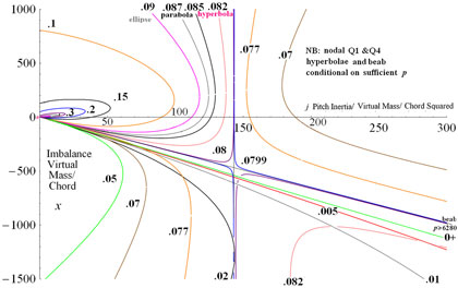
 ${{\boldsymbol{x}}} = -676$
and
${{\boldsymbol{x}}} = -676$
and
 ${\boldsymbol{j}} = 487$
for the minimum P of 4800 (vs
${\boldsymbol{j}} = 487$
for the minimum P of 4800 (vs
 ${\boldsymbol{x}}^{2}/{\boldsymbol{j}} = 938$
) (with
${\boldsymbol{x}}^{2}/{\boldsymbol{j}} = 938$
) (with
 ${\boldsymbol{e}} =.15$
and
${\boldsymbol{e}} =.15$
and
 ${\boldsymbol{x}}_{\textbf{z}} =-275$
,
${\boldsymbol{x}}_{\textbf{z}} =-275$
,
 ${\boldsymbol{k}}_{\textbf{z}}=.054$
)
${\boldsymbol{k}}_{\textbf{z}}=.054$
)
For
 ${\boldsymbol{k}}\neq {{\boldsymbol{k}}}_{\textbf{z}}$
multiply (18) by
${\boldsymbol{k}}\neq {{\boldsymbol{k}}}_{\textbf{z}}$
multiply (18) by
 ${\boldsymbol{\beta}} \boldsymbol\neq \boldsymbol{0}$
(so
${\boldsymbol{\beta}} \boldsymbol\neq \boldsymbol{0}$
(so
 $[\underline{\text{A}},\underline{\text{B}}]_{0} \neq 0$
) to eliminate
$[\underline{\text{A}},\underline{\text{B}}]_{0} \neq 0$
) to eliminate
 ${\boldsymbol{k}}_{\textbf{n}}^{2}$
(by 19) from even power real terms.
${\boldsymbol{k}}_{\textbf{n}}^{2}$
(by 19) from even power real terms.
 \begin{equation}
({\chi-\alpha}\textit{k}^{2})[\underline{\text{A}},\underline{\text{B}}]=(| \underline{\text{B}}| +[\underline{\text{A}},\underline{\text{C}}]-| \underline{\text{A}}| \textit{k}^{2})\beta
\label{eqn28}
\end{equation}
\begin{equation}
({\chi-\alpha}\textit{k}^{2})[\underline{\text{A}},\underline{\text{B}}]=(| \underline{\text{B}}| +[\underline{\text{A}},\underline{\text{C}}]-| \underline{\text{A}}| \textit{k}^{2})\beta
\label{eqn28}
\end{equation}
with a
 ${{\boldsymbol{k}}}^{\textbf{2}}$
factored out. Look for other
${{\boldsymbol{k}}}^{\textbf{2}}$
factored out. Look for other
 ${{\boldsymbol{k}}}\boldsymbol\neq {{\boldsymbol{k}}}_{{\boldsymbol{z}}}$
solutions on
${{\boldsymbol{k}}}\boldsymbol\neq {{\boldsymbol{k}}}_{{\boldsymbol{z}}}$
solutions on
 ${\boldsymbol{j}}_{{\boldsymbol{z}}}$
with
${\boldsymbol{j}}_{{\boldsymbol{z}}}$
with
 ${\boldsymbol{\alpha}}{\,\boldsymbol\approx\,}{\boldsymbol{j}}_{{\boldsymbol{z}}}$
so
${\boldsymbol{\alpha}}{\,\boldsymbol\approx\,}{\boldsymbol{j}}_{{\boldsymbol{z}}}$
so
 $\boldsymbol{(k}_{\textbf{z}}^{\textbf{2}}{\boldsymbol{-k}}^{\textbf{2}}){\boldsymbol{j}}_{{\boldsymbol{z}}}[\underline{\text{A}},\underline{\text{B}}] = \{\underline{\text{B}}| \textbf{+}[\underline{\text{A}},\underline{\text{C}}]\textbf{-}|\underline{\text{A}}| {\boldsymbol{k}}^{2}\}\boldsymbol{(k-k}_{\textbf{z}}{\textbf{)}}\textbf{d} {\boldsymbol{\beta}}/\textbf{d}{\boldsymbol{k}}$
or
$\boldsymbol{(k}_{\textbf{z}}^{\textbf{2}}{\boldsymbol{-k}}^{\textbf{2}}){\boldsymbol{j}}_{{\boldsymbol{z}}}[\underline{\text{A}},\underline{\text{B}}] = \{\underline{\text{B}}| \textbf{+}[\underline{\text{A}},\underline{\text{C}}]\textbf{-}|\underline{\text{A}}| {\boldsymbol{k}}^{2}\}\boldsymbol{(k-k}_{\textbf{z}}{\textbf{)}}\textbf{d} {\boldsymbol{\beta}}/\textbf{d}{\boldsymbol{k}}$
or
 $\boldsymbol{(k}_{{\boldsymbol{z}}}{\boldsymbol{+k}}\textbf{)}{\boldsymbol{j}}_{{\boldsymbol{z}}}[\underline{\text{A}},\underline{\text{B}}] \cong {\boldsymbol{e}}\{| \underline{\text{B}}| \textbf{+}[\underline{\text{A}},\underline{\text{C}}]\textbf{-}|\underline{\text{A}}| {\boldsymbol{k}}^{\textbf{2}}\}(\pi{\boldsymbol{q}}+4\textbf{d}{\boldsymbol{g}}/\textbf{d}{\boldsymbol{k}}\textbf{)}$
via 6. Using again
$\boldsymbol{(k}_{{\boldsymbol{z}}}{\boldsymbol{+k}}\textbf{)}{\boldsymbol{j}}_{{\boldsymbol{z}}}[\underline{\text{A}},\underline{\text{B}}] \cong {\boldsymbol{e}}\{| \underline{\text{B}}| \textbf{+}[\underline{\text{A}},\underline{\text{C}}]\textbf{-}|\underline{\text{A}}| {\boldsymbol{k}}^{\textbf{2}}\}(\pi{\boldsymbol{q}}+4\textbf{d}{\boldsymbol{g}}/\textbf{d}{\boldsymbol{k}}\textbf{)}$
via 6. Using again
 ${\boldsymbol{p}} = 0, | \underline{\text{B}}| \textbf{+}[\underline{\text{A}},\underline{\text{C}}]\boldsymbol{-k}_{{\boldsymbol{z}}}^{\textbf{2}} | \underline{\text{A}} | > 0 > 4 {\textbf{d}} {\boldsymbol{g}}/\textbf{d} {\boldsymbol{k}}$
which dominates
${\boldsymbol{p}} = 0, | \underline{\text{B}}| \textbf{+}[\underline{\text{A}},\underline{\text{C}}]\boldsymbol{-k}_{{\boldsymbol{z}}}^{\textbf{2}} | \underline{\text{A}} | > 0 > 4 {\textbf{d}} {\boldsymbol{g}}/\textbf{d} {\boldsymbol{k}}$
which dominates
 $\boldsymbol\pi{\boldsymbol{q}}$
at negative
$\boldsymbol\pi{\boldsymbol{q}}$
at negative
 ${\boldsymbol{x}}_{\boldsymbol{z}}$
, then such intersections only exist for negative [A, B]. So as k increases from
${\boldsymbol{x}}_{\boldsymbol{z}}$
, then such intersections only exist for negative [A, B]. So as k increases from
 ${\boldsymbol{k}}_{\boldsymbol{z}}$
, the contours increasingly above the beab line are simply nested inside the
${\boldsymbol{k}}_{\boldsymbol{z}}$
, the contours increasingly above the beab line are simply nested inside the
 ${\boldsymbol{k}}_{\boldsymbol{z}}^{+}$
contour which must asymptote to
${\boldsymbol{k}}_{\boldsymbol{z}}^{+}$
contour which must asymptote to
 ${\boldsymbol{j}} = {\boldsymbol{j}}_{{\boldsymbol{z}}}$
Diagonal mirror hyperbolae roughly about the node will also be viable in nodal quadrant 4 “Q4” at sufficient
${\boldsymbol{j}} = {\boldsymbol{j}}_{{\boldsymbol{z}}}$
Diagonal mirror hyperbolae roughly about the node will also be viable in nodal quadrant 4 “Q4” at sufficient
 ${\boldsymbol{p}} > {{\boldsymbol{P}}} + 1$
to overcome negative
${\boldsymbol{p}} > {{\boldsymbol{P}}} + 1$
to overcome negative
 $[\underline{\text{A}},\underline{\text{B}}]_{0}$
to get the same+ sign as such
$[\underline{\text{A}},\underline{\text{B}}]_{0}$
to get the same+ sign as such
 ${\boldsymbol{\beta}}$
(though may (Fig. 6) slightly intersect
${\boldsymbol{\beta}}$
(though may (Fig. 6) slightly intersect
 ${\boldsymbol{j}} = {\boldsymbol{j}}_{{\boldsymbol{z}}}$
).
${\boldsymbol{j}} = {\boldsymbol{j}}_{{\boldsymbol{z}}}$
).
Figure 6. Low k contours in the macro inertia imbalance plane for
 ${\boldsymbol{e}}=.15$
 ${\boldsymbol{k}}_{{\boldsymbol{z}}} =.054$
.
${\boldsymbol{k}}_{{\boldsymbol{z}}} =.054$
.
So at
 ${\boldsymbol{p}} = 0$
and below the node
${\boldsymbol{p}} = 0$
and below the node
 ${\boldsymbol{k}}_{\boldsymbol{z}} [\underline{\text{A}},\underline{\text{B}}]_{0} \textbf{=} 4\Delta \{{\boldsymbol{Fj}}_{\boldsymbol{z}} + ({g}\boldsymbol{-Fq+Fy)}{\boldsymbol{x}}\}-{\textbf{1}}/{\textbf{2}}{\boldsymbol{g}}\} \,\approx\, \textbf{4}\Delta\{\textbf{(}{g}\boldsymbol{-Fq+Fy)}{\boldsymbol{x}}\}$
and
${\boldsymbol{k}}_{\boldsymbol{z}} [\underline{\text{A}},\underline{\text{B}}]_{0} \textbf{=} 4\Delta \{{\boldsymbol{Fj}}_{\boldsymbol{z}} + ({g}\boldsymbol{-Fq+Fy)}{\boldsymbol{x}}\}-{\textbf{1}}/{\textbf{2}}{\boldsymbol{g}}\} \,\approx\, \textbf{4}\Delta\{\textbf{(}{g}\boldsymbol{-Fq+Fy)}{\boldsymbol{x}}\}$
and
 $| \underline{\text{B}} | \textbf{+}[\underline{\text{A}},\underline{\text{C}}]\textbf{-}|\underline{\text{A}}| {\boldsymbol{k}}^{\textbf{2}} \,\approx\, -4{{\boldsymbol{Fx}+\textit{k}}}^{\textbf{2}} {\boldsymbol{x}}^{\textbf{2}}$
again which combined give a quadratic eqn in x
$| \underline{\text{B}} | \textbf{+}[\underline{\text{A}},\underline{\text{C}}]\textbf{-}|\underline{\text{A}}| {\boldsymbol{k}}^{\textbf{2}} \,\approx\, -4{{\boldsymbol{Fx}+\textit{k}}}^{\textbf{2}} {\boldsymbol{x}}^{\textbf{2}}$
again which combined give a quadratic eqn in x
 \begin{equation}
k^{2}x^{2}-4Fx=4(k_{z}+k)j_{z}\Delta\{(g-Fq+Fy)x\}/(\pi q+4 \textbf{d}\boldsymbol{g}/\textbf{d}\boldsymbol{k})
\label{eqn29}
\end{equation}
\begin{equation}
k^{2}x^{2}-4Fx=4(k_{z}+k)j_{z}\Delta\{(g-Fq+Fy)x\}/(\pi q+4 \textbf{d}\boldsymbol{g}/\textbf{d}\boldsymbol{k})
\label{eqn29}
\end{equation}
For
 ${\boldsymbol{e}} =.15$
 ${\boldsymbol{k}}_{z} =.054$
 ${\boldsymbol{g}}_{z} = 1.697$
 ${\boldsymbol{F}} = .951$
 ${\boldsymbol{j}}_{\boldsymbol{z}} = 198$
nodal
${\boldsymbol{j}}_{\boldsymbol{z}} = 198$
nodal
 ${\boldsymbol{x}}_{\boldsymbol{z}}= -275$
there is no real root at
${\boldsymbol{x}}_{\boldsymbol{z}}= -275$
there is no real root at
 ${\boldsymbol{k}} = {\boldsymbol{k}}_{\boldsymbol{z}}^{-}$
as per a downwards asymptote but an intersection at
${\boldsymbol{k}} = {\boldsymbol{k}}_{\boldsymbol{z}}^{-}$
as per a downwards asymptote but an intersection at
 ${\boldsymbol{k}} =.95{\boldsymbol{k}}_{{\boldsymbol{z}}}$
at
${\boldsymbol{k}} =.95{\boldsymbol{k}}_{{\boldsymbol{z}}}$
at
 $\boldsymbol{ {x}} = -740$
; and by
$\boldsymbol{ {x}} = -740$
; and by
 ${\boldsymbol{k}} = .9{\boldsymbol{k}}_{\boldsymbol{z}}$
 ${\boldsymbol{g}}=1.762$
 ${\boldsymbol{F}}=.956$
give
${\boldsymbol{F}}=.956$
give
 ${\boldsymbol{k}}^{\textbf{2}} {\boldsymbol{x}}^{\textbf{2}} + 4.96{\boldsymbol{x}} + 2234 = 0$
for
${\boldsymbol{k}}^{\textbf{2}} {\boldsymbol{x}}^{\textbf{2}} + 4.96{\boldsymbol{x}} + 2234 = 0$
for
 ${\boldsymbol{x}} = -654$
and -1444. This agrees roughly with evaluation in Fig. 6 of the exact solution (29) below which shows the
${\boldsymbol{x}} = -654$
and -1444. This agrees roughly with evaluation in Fig. 6 of the exact solution (29) below which shows the
 ${\boldsymbol{k}} = .05$
contour intercepts at about
${\boldsymbol{k}} = .05$
contour intercepts at about
 $-700$
and on a bigger scale then bends back. The smaller roots move upwards as k is further reduced to crowd the intercept of qs line. So the
$-700$
and on a bigger scale then bends back. The smaller roots move upwards as k is further reduced to crowd the intercept of qs line. So the
 $0 \lt {\boldsymbol{k}} \lt {\boldsymbol{k}}_{\boldsymbol{z}}$
contours are not nested but all cross each other and the qs line between the nexus and
$0 \lt {\boldsymbol{k}} \lt {\boldsymbol{k}}_{\boldsymbol{z}}$
contours are not nested but all cross each other and the qs line between the nexus and
 ${\boldsymbol{j}}_{z}$
to invert their order! Note their nodal quadrant 1 (eg
${\boldsymbol{j}}_{z}$
to invert their order! Note their nodal quadrant 1 (eg
 ${\boldsymbol{k}} = .05$
) mirror hyperbolae like the beab line and quadrant 4 hyperbolae have label gaps to indicate severe conditionality on (27):
${\boldsymbol{k}} = .05$
) mirror hyperbolae like the beab line and quadrant 4 hyperbolae have label gaps to indicate severe conditionality on (27):
 \begin{equation}
k^{2} = \chi[\underline{\text{A}},\underline{\text{B}}]{-}(|\underline{\text{B}}|{+}[\underline{\text{A}},\underline{\text{C}}])\beta\ /\ \mathrm{\alpha[\underline{\text{A}},\underline{\text{B}}]}-|\underline{\text{A}}| \beta
\label{eqn30}
\end{equation}
\begin{equation}
k^{2} = \chi[\underline{\text{A}},\underline{\text{B}}]{-}(|\underline{\text{B}}|{+}[\underline{\text{A}},\underline{\text{C}}])\beta\ /\ \mathrm{\alpha[\underline{\text{A}},\underline{\text{B}}]}-|\underline{\text{A}}| \beta
\label{eqn30}
\end{equation}
The general exact (Routh) neutral stability criterion is from (29)
 \begin{equation}
{\chi}{[\underline{\text{A}},\underline{\text{B}}]-}{{\beta}}(|\underline{\text{B}}| +[\underline{\text{A}},\underline{\text{C}}]) = 8F^{2}\{2ej+(y-2eq)x-qy\}
\label{eqn31}
\end{equation}
\begin{equation}
{\chi}{[\underline{\text{A}},\underline{\text{B}}]-}{{\beta}}(|\underline{\text{B}}| +[\underline{\text{A}},\underline{\text{C}}]) = 8F^{2}\{2ej+(y-2eq)x-qy\}
\label{eqn31}
\end{equation}
Fortunately the numerator in (32) has only a term in g in each product, for easy calculation by hand which shows the two (singular at
 ${\boldsymbol{k}} = 0$
) g terms cancel exactly as do the p terms so as before (1) the numerator is the linear
${\boldsymbol{k}} = 0$
) g terms cancel exactly as do the p terms so as before (1) the numerator is the linear
 \begin{equation}
ej+({1}/{8}/F-e^{2})x = qy/2
\label{eqn32}
\end{equation}
\begin{equation}
ej+({1}/{8}/F-e^{2})x = qy/2
\label{eqn32}
\end{equation}
Note
 $\{\}=0$
is the
$\{\}=0$
is the
 ${\boldsymbol{\beta}}=[\alpha,\beta]=0$
beab line (28) at
${\boldsymbol{\beta}}=[\alpha,\beta]=0$
beab line (28) at
 ${\boldsymbol{k}} = {\boldsymbol{k}}_{z}$
and generally the small k lines
${\boldsymbol{k}} = {\boldsymbol{k}}_{z}$
and generally the small k lines
 \begin{align}
\alpha[\underline{\text{A}},\underline{\text{B}}]-\beta|\underline{\text{A}}| =4F(j-qx)(j-yx) -4g\{(4g-1)e(j-ex) -(j-e-{1}/{4})x+e(x^{2}-2gq)\}
\label{eqn33}
\end{align}
\begin{align}
\alpha[\underline{\text{A}},\underline{\text{B}}]-\beta|\underline{\text{A}}| =4F(j-qx)(j-yx) -4g\{(4g-1)e(j-ex) -(j-e-{1}/{4})x+e(x^{2}-2gq)\}
\label{eqn33}
\end{align}
through the nexus, with
 ${\boldsymbol{k}} = 0$
 ${\boldsymbol{F}} = 1$
the qs. line. Also for
${\boldsymbol{F}} = 1$
the qs. line. Also for
 $\{\} = 0$
 ${\boldsymbol{P}}+1\textbf{=}-[\underline{\text{A}},\underline{\text{B}}]_{0/}{\boldsymbol{\beta}}=-(|\underline{\text{B}}| \textbf{+}[\underline{\text{A}},\underline{\text{C}}])/\boldsymbol{\chi}=({\boldsymbol{x}-}{1}/{2})\boldsymbol{/e}$
still unaffected by small k, let alone G. Or
${\boldsymbol{P}}+1\textbf{=}-[\underline{\text{A}},\underline{\text{B}}]_{0/}{\boldsymbol{\beta}}=-(|\underline{\text{B}}| \textbf{+}[\underline{\text{A}},\underline{\text{C}}])/\boldsymbol{\chi}=({\boldsymbol{x}-}{1}/{2})\boldsymbol{/e}$
still unaffected by small k, let alone G. Or
 ${\boldsymbol{eP}=\textit{x-q}}$
. The denominator in (32) needs
${\boldsymbol{eP}=\textit{x-q}}$
. The denominator in (32) needs
 ${\boldsymbol{p}} = 0$
to avoid working lengthy p terms which eventually cancel anyways. So lightening the algebra gives
${\boldsymbol{p}} = 0$
to avoid working lengthy p terms which eventually cancel anyways. So lightening the algebra gives
 \begin{equation}
{1}/{4}/F\ \mathrm{of}\ j[\underline{\text{A}},\underline{\text{B}}]_{0} + \beta x^{2}\ \mathrm{as}\ 1/F\ \mathrm{of}\ Fj^{2} + (g-F(q+y))jx +(Fqy-eg)x^{2} - {1}/{2}k^{2}jg/F
\label{eqn34}
\end{equation}
\begin{equation}
{1}/{4}/F\ \mathrm{of}\ j[\underline{\text{A}},\underline{\text{B}}]_{0} + \beta x^{2}\ \mathrm{as}\ 1/F\ \mathrm{of}\ Fj^{2} + (g-F(q+y))jx +(Fqy-eg)x^{2} - {1}/{2}k^{2}jg/F
\label{eqn34}
\end{equation}
A vital check is that its new g and
 ${\boldsymbol{g}}^{2}$
terms do vanish at the nexus
${\boldsymbol{g}}^{2}$
terms do vanish at the nexus
 $\boldsymbol{\mathcal{N}}\ {\boldsymbol{j=q}}^{2}$
 ${\boldsymbol{x=q}}$
since
${\boldsymbol{x=q}}$
since
 ${\boldsymbol{e}} = {\boldsymbol{q}}-{1}/{2}$
, so again whatever the T both numerator and denominator vanish there, so all k contours pass through it(Reference Farthing7).
${\boldsymbol{e}} = {\boldsymbol{q}}-{1}/{2}$
, so again whatever the T both numerator and denominator vanish there, so all k contours pass through it(Reference Farthing7).
 $\textbf{4}{\boldsymbol{g}} > 1$
for
$\textbf{4}{\boldsymbol{g}} > 1$
for
 ${\boldsymbol{k}} \lt .6$
but generally the two
${\boldsymbol{k}} \lt .6$
but generally the two
 ${\boldsymbol{eg}}^{2}$
terms will prove of little impact, the first being linear in j and x and the second constant. For small k they do lead on the RHS at
${\boldsymbol{eg}}^{2}$
terms will prove of little impact, the first being linear in j and x and the second constant. For small k they do lead on the RHS at
 ${\boldsymbol{e}} \mathrm{O} (\mathrm{Ln}{\boldsymbol{k}})^{2}$
followed by the non-linear jx and
${\boldsymbol{e}} \mathrm{O} (\mathrm{Ln}{\boldsymbol{k}})^{2}$
followed by the non-linear jx and
 ${\boldsymbol{x}}^{\boldsymbol{2}}\mathrm{O}(\mathrm{Ln}{\boldsymbol{k}})\boldsymbol{g}$
terms. Substituting (33) and (35) in (32) and dividing though by 4F,
${\boldsymbol{x}}^{\boldsymbol{2}}\mathrm{O}(\mathrm{Ln}{\boldsymbol{k}})\boldsymbol{g}$
terms. Substituting (33) and (35) in (32) and dividing though by 4F,
 \begin{equation}
k^{4}\delta = 4\textit{F}^{2}\sigma
\label{eqn35}
\end{equation}
\begin{equation}
k^{4}\delta = 4\textit{F}^{2}\sigma
\label{eqn35}
\end{equation}
where the
 ${\boldsymbol{k}}^{2}$
multiplying the denominator has shifted the singular g and
${\boldsymbol{k}}^{2}$
multiplying the denominator has shifted the singular g and
 ${\boldsymbol{g}}^{2}$
terms back to finite G and
${\boldsymbol{g}}^{2}$
terms back to finite G and
 ${\boldsymbol{G}}^{2}$
terms. So correct to first order in k, the contours do radiate linearly from the nexus as the LHS{} =0 or as (34).
${\boldsymbol{G}}^{2}$
terms. So correct to first order in k, the contours do radiate linearly from the nexus as the LHS{} =0 or as (34).
At a given k (36) is a conic section in the variables x and j. The discriminant
 $\sigma=$
squared coefficient of xj - 4 coefficient of
$\sigma=$
squared coefficient of xj - 4 coefficient of
 ${\boldsymbol{j}}^{2}$
by coefficient of x
${\boldsymbol{j}}^{2}$
by coefficient of x
 ${}^{2}$
in (36), which all come from the denominator (35) as
${}^{2}$
in (36), which all come from the denominator (35) as
 \begin{align}
{1}/{4}{x}^{2}\beta\mathrm{/F} &- {x}[{1}/{2}-4{e}^{2}{F + jk}^{2}({q+y}) - \{{e}^{2}(4{G-k})+({j-e}-{1}/{4}){k}\}{G/F}] \nonumber\\[2pt]
&+{j}^{2}{k}^{2} -4{ejF}+2{Fqy} + {e}\{2{qG}+{j}({k}-4{G})\}{G/F} =0
\label{eqn36}\end{align}
\begin{align}
{1}/{4}{x}^{2}\beta\mathrm{/F} &- {x}[{1}/{2}-4{e}^{2}{F + jk}^{2}({q+y}) - \{{e}^{2}(4{G-k})+({j-e}-{1}/{4}){k}\}{G/F}] \nonumber\\[2pt]
&+{j}^{2}{k}^{2} -4{ejF}+2{Fqy} + {e}\{2{qG}+{j}({k}-4{G})\}{G/F} =0
\label{eqn36}\end{align}
So
 $F^{2} \sigma/k^{4} = (g-Fq-Fy)^{2}-4F(Fqy-ge) = g^{2} + (Fq-Fy)^{2} + 2gF (2e-q-y) = g^{2} - 2g ({1}/{2}F + {1}/{4}) + ({1}/{2} F-{1}/{4})^{2}$
with all e dependence having cancelled.
$F^{2} \sigma/k^{4} = (g-Fq-Fy)^{2}-4F(Fqy-ge) = g^{2} + (Fq-Fy)^{2} + 2gF (2e-q-y) = g^{2} - 2g ({1}/{2}F + {1}/{4}) + ({1}/{2} F-{1}/{4})^{2}$
with all e dependence having cancelled.
Completing the square
 ${\boldsymbol{F}}^{\textbf 2}\sigma /{\boldsymbol{k}}^{\textbf{4}} \textbf{=} {\boldsymbol{g}}^{\textbf 2} \textbf{-}\textbf{2}{\boldsymbol{g}} \textbf{(}{\textbf 1}/{\textbf 2}{\boldsymbol{F}}\textbf{+}{\textbf 1}/{\textbf 4}\textbf{)+(}{\textbf{1}}/{\textbf{2}}{\boldsymbol{F}}\textbf{+}{\textbf{1}}/{\textbf{4}}\textbf{)}^{\textbf{2}} \textbf{-} {\textbf{1}}/{\textbf{2}}{\boldsymbol{F}} \textbf{=} \textbf{(}{\boldsymbol{g}}\textbf{-}{\textbf{1}}/{\textbf{2}}{\boldsymbol{F}}\textbf{-}{\textbf{1}}/{\textbf{4}}\textbf{)}^{\textbf{2}}\textbf{-}{\textbf{1}}/{\textbf{2}}{\boldsymbol{F,}}$
the same as
${\boldsymbol{F}}^{\textbf 2}\sigma /{\boldsymbol{k}}^{\textbf{4}} \textbf{=} {\boldsymbol{g}}^{\textbf 2} \textbf{-}\textbf{2}{\boldsymbol{g}} \textbf{(}{\textbf 1}/{\textbf 2}{\boldsymbol{F}}\textbf{+}{\textbf 1}/{\textbf 4}\textbf{)+(}{\textbf{1}}/{\textbf{2}}{\boldsymbol{F}}\textbf{+}{\textbf{1}}/{\textbf{4}}\textbf{)}^{\textbf{2}} \textbf{-} {\textbf{1}}/{\textbf{2}}{\boldsymbol{F}} \textbf{=} \textbf{(}{\boldsymbol{g}}\textbf{-}{\textbf{1}}/{\textbf{2}}{\boldsymbol{F}}\textbf{-}{\textbf{1}}/{\textbf{4}}\textbf{)}^{\textbf{2}}\textbf{-}{\textbf{1}}/{\textbf{2}}{\boldsymbol{F,}}$
the same as
 $\textbf{{1}/{4}}$
of
$\textbf{{1}/{4}}$
of
 $\mathbf\delta = \boldsymbol{((2g-F} \textbf{-}{\textbf{1}}/{\textbf{2}}\textbf{)}^{\textbf{2}}\textbf{-} \textbf{2}{\boldsymbol{F}}$
in (11) so
$\mathbf\delta = \boldsymbol{((2g-F} \textbf{-}{\textbf{1}}/{\textbf{2}}\textbf{)}^{\textbf{2}}\textbf{-} \textbf{2}{\boldsymbol{F}}$
in (11) so
 \begin{equation}
x^{2}k^{2}/ 32F-x[{1}/{2}+jk^{2}(q+y)-(j-{1}/{4})kG/F]+j^{2}k^{2}+{1}/{4} \cong 0
\label{eqn37}
\end{equation}
\begin{equation}
x^{2}k^{2}/ 32F-x[{1}/{2}+jk^{2}(q+y)-(j-{1}/{4})kG/F]+j^{2}k^{2}+{1}/{4} \cong 0
\label{eqn37}
\end{equation}
and the crossover k of zero discriminant and parabolic contour is thus the same
 ${\boldsymbol{k}}_{\boldsymbol{c}} = .087$
 $\delta = 0$
maximum k for unitary flutter. Thus the computed Q4 mirror hyperbolae stop before this
$\delta = 0$
maximum k for unitary flutter. Thus the computed Q4 mirror hyperbolae stop before this
 ${\boldsymbol{k}}_{\boldsymbol{c}}$
in all plots. It is superficially stunning that the discriminant
${\boldsymbol{k}}_{\boldsymbol{c}}$
in all plots. It is superficially stunning that the discriminant
 $\delta$
of the quadratic eqn
$\delta$
of the quadratic eqn
 ${\boldsymbol\beta} =0$
in e (and no x or j) is proportional to the discriminant
${\boldsymbol\beta} =0$
in e (and no x or j) is proportional to the discriminant
 $\sigma$
of the quadratic in j and x for binary flutter originating from the
$\sigma$
of the quadratic in j and x for binary flutter originating from the
 $[\underline{\text{A}},\underline{\text{B}}]{\boldsymbol{\alpha}}\textbf{-}{\boldsymbol{\beta}}|\underline{\text{A}}|$
in (35).
$[\underline{\text{A}},\underline{\text{B}}]{\boldsymbol{\alpha}}\textbf{-}{\boldsymbol{\beta}}|\underline{\text{A}}|$
in (35).
 ${\boldsymbol{k}}_{\boldsymbol{c}} \geq {\boldsymbol{k}}_{z}$
is the upper limit of
${\boldsymbol{k}}_{\boldsymbol{c}} \geq {\boldsymbol{k}}_{z}$
is the upper limit of
 ${\boldsymbol{k}}_{z}$
for big enough g to neutralise the real pitch damping to allow unitary flutter, whilst binarily it is the k at which the contours in x,j space lose the hyperbolic influence of unitary flutter at
${\boldsymbol{k}}_{z}$
for big enough g to neutralise the real pitch damping to allow unitary flutter, whilst binarily it is the k at which the contours in x,j space lose the hyperbolic influence of unitary flutter at
 ${\boldsymbol{k}}_{\boldsymbol{z}}$
and become elliptic.
${\boldsymbol{k}}_{\boldsymbol{z}}$
and become elliptic.
With (5)
 ${\boldsymbol{F}} \,\approx\, {\textbf 1}/{\textbf 2} \textbf{+} {\textbf 1}/{\textbf 4} {\boldsymbol{k}}^{-2}{\boldsymbol{,}}$
and no g,
${\boldsymbol{F}} \,\approx\, {\textbf 1}/{\textbf 2} \textbf{+} {\textbf 1}/{\textbf 4} {\boldsymbol{k}}^{-2}{\boldsymbol{,}}$
and no g,
 $\sigma\downarrow 1/64$
as
$\sigma\downarrow 1/64$
as
 ${\boldsymbol{k}} \uparrow \infty$
hyperbolic approaching parabolic about the pure
${\boldsymbol{k}} \uparrow \infty$
hyperbolic approaching parabolic about the pure
 ${3}/{4}$
pitch infinite k ray or by (12)
${3}/{4}$
pitch infinite k ray or by (12)
 $\boldsymbol{\delta} = 0$
when
$\boldsymbol{\delta} = 0$
when
 ${\boldsymbol{F}} = {1}/{2}$
if g is ignored. If not, as
${\boldsymbol{F}} = {1}/{2}$
if g is ignored. If not, as
 ${\boldsymbol{k}} \uparrow \infty, \ {\boldsymbol{F}}^{\textbf{2}}\sigma /{\boldsymbol{k}}^{\textbf{4}} \,\approx\, \boldsymbol{-2g}({\textbf{1}}/{\textbf{2}} {\boldsymbol{F}}\textbf{+}{\textbf 1}/{\textbf 4}) \,\approx\, {\boldsymbol{g}}$
so with
${\boldsymbol{k}} \uparrow \infty, \ {\boldsymbol{F}}^{\textbf{2}}\sigma /{\boldsymbol{k}}^{\textbf{4}} \,\approx\, \boldsymbol{-2g}({\textbf{1}}/{\textbf{2}} {\boldsymbol{F}}\textbf{+}{\textbf 1}/{\textbf 4}) \,\approx\, {\boldsymbol{g}}$
so with
 ${\boldsymbol{Gk}} \uparrow {1}/{4}, \, \sigma/{\boldsymbol{k}}^{2}\downarrow-{\boldsymbol{Gk}}/{\boldsymbol{F}}^2\downarrow-1$
. G damps
${\boldsymbol{Gk}} \uparrow {1}/{4}, \, \sigma/{\boldsymbol{k}}^{2}\downarrow-{\boldsymbol{Gk}}/{\boldsymbol{F}}^2\downarrow-1$
. G damps
 ${3}/{4}$
pitch to close the real F high k hyperbolic contours into ellipses. In all eg has completely changed the topology of the contours as even the remaining
${3}/{4}$
pitch to close the real F high k hyperbolic contours into ellipses. In all eg has completely changed the topology of the contours as even the remaining
 ${\boldsymbol{k}} \leq {\boldsymbol{k}}_{\boldsymbol{c}}$
hyperbolic contours have shifted their conic center from negative x and j to the pure-pitch node. Now for generating the contours collect the powers of x in (33) to form its quadratic
${\boldsymbol{k}} \leq {\boldsymbol{k}}_{\boldsymbol{c}}$
hyperbolic contours have shifted their conic center from negative x and j to the pure-pitch node. Now for generating the contours collect the powers of x in (33) to form its quadratic
 \begin{equation}
{{D}}=g/F-q-y,\ {\text{then}}\ \ 2F\{2ej+(y-2eq)x-qy\} \,\approx\, k^{2}j(j+x{\texttt{D}})+{1}/{4}x^{2}k^{2} \beta/F .
\label{eqn38}
\end{equation}
\begin{equation}
{{D}}=g/F-q-y,\ {\text{then}}\ \ 2F\{2ej+(y-2eq)x-qy\} \,\approx\, k^{2}j(j+x{\texttt{D}})+{1}/{4}x^{2}k^{2} \beta/F .
\label{eqn38}
\end{equation}
Then steps in j and k and thus F(k) and G(k) and y(F) give the stability contours of k at a given e in j,x space. So the entire flutter onset frequency k and its modes can be calculated exactly without iterative solution or interpolating for contours. The upper and lower x root contours join vertically where their curvature is then
 $\mathrm{d}^{2}{\boldsymbol{j}/}\mathrm{d}{\boldsymbol{x}}^{2}$
proportional to
$\mathrm{d}^{2}{\boldsymbol{j}/}\mathrm{d}{\boldsymbol{x}}^{2}$
proportional to
 ${\boldsymbol{\beta}}$
again implying the
${\boldsymbol{\beta}}$
again implying the
 ${\boldsymbol{k}}\rightarrow {\boldsymbol{k}}_{\boldsymbol{z}}$
and
${\boldsymbol{k}}\rightarrow {\boldsymbol{k}}_{\boldsymbol{z}}$
and
 ${\boldsymbol{\beta}} \rightarrow \textbf{0}$
are flat asymptotes to the vertical line
${\boldsymbol{\beta}} \rightarrow \textbf{0}$
are flat asymptotes to the vertical line
 ${\boldsymbol{j}} \uparrow {\boldsymbol{j}}_{\boldsymbol{z}}$
.
${\boldsymbol{j}} \uparrow {\boldsymbol{j}}_{\boldsymbol{z}}$
.
4.0 APPROXIMATIONS AND CALCULATIONS OF THE FULL BINARY SOLUTION
At aerodynamic balance
 ${{\boldsymbol{e}}} \cong 0$
, q = 1/2, Fy=1/4,
${{\boldsymbol{e}}} \cong 0$
, q = 1/2, Fy=1/4,
 ${\boldsymbol{\beta}}$
=Fqy = 1/8 the only coefficient with a G term is in the middle ‘b’ term of the quadratic (39)
${\boldsymbol{\beta}}$
=Fqy = 1/8 the only coefficient with a G term is in the middle ‘b’ term of the quadratic (39)
 \begin{equation}
4\textit{Fej}+\textit{x}({1}/{2}-4\textit{Fe}^{2})\cong\textit{ jxk}{}^{2}{\texttt{D}} +{1}/{4}\textit{x}{}^{2}\textit{k}^{2}\beta/\textit{F} .
\label{eqn39}
\end{equation}
\begin{equation}
4\textit{Fej}+\textit{x}({1}/{2}-4\textit{Fe}^{2})\cong\textit{ jxk}{}^{2}{\texttt{D}} +{1}/{4}\textit{x}{}^{2}\textit{k}^{2}\beta/\textit{F} .
\label{eqn39}
\end{equation}
 ${{\boldsymbol{j}}}-{1}/{4}$
is here the j distance to the nexal
${{\boldsymbol{j}}}-{1}/{4}$
is here the j distance to the nexal
 ${{\boldsymbol{j}}}= {1}/{4}$
. So G times it decreases of the magnitude of the x coefficient b, which increases the lower root
${{\boldsymbol{j}}}= {1}/{4}$
. So G times it decreases of the magnitude of the x coefficient b, which increases the lower root
 $\cong$
c/b and decreases the upper root
$\cong$
c/b and decreases the upper root
 $\cong$
b/a bringing the roots closer together. Both tie in with the upper and lower contours being joined by G. Now at small
$\cong$
b/a bringing the roots closer together. Both tie in with the upper and lower contours being joined by G. Now at small
 ${\boldsymbol{k}}$
, (6)
${\boldsymbol{k}}$
, (6)
 ${\boldsymbol{F}} \rightarrow \textbf{1}-{\textbf{1}}/{\textbf{4}}{\boldsymbol\pi}{\boldsymbol{k}}$
,
${\boldsymbol{F}} \rightarrow \textbf{1}-{\textbf{1}}/{\textbf{4}}{\boldsymbol\pi}{\boldsymbol{k}}$
,
 ${\boldsymbol{G}} \uparrow \boldsymbol{-{1}/{2}k Ln}({1}/{2}{\boldsymbol{k}})$
so
${\boldsymbol{G}} \uparrow \boldsymbol{-{1}/{2}k Ln}({1}/{2}{\boldsymbol{k}})$
so
 ${{\boldsymbol{x}}} = {1}/{2}- {1}/{2}({\boldsymbol{j}}-{1}/{4})$
k
${{\boldsymbol{x}}} = {1}/{2}- {1}/{2}({\boldsymbol{j}}-{1}/{4})$
k
 ${}^{\textbf{2}}$
Ln(
${}^{\textbf{2}}$
Ln(
 ${1}/{2}{\boldsymbol{k}}$
) +O(k
${1}/{2}{\boldsymbol{k}}$
) +O(k
 ${}^{\textbf{2}}$
) so G leads in the spacing of the (first) contours.
${}^{\textbf{2}}$
) so G leads in the spacing of the (first) contours.
Now
 ${\boldsymbol{e}} > 0$
introduces ej in the qs. line equation (34) so it slopes downward and offshoots from the nexus new lines with slopes reducing linearly with small k such as the beab line at
${\boldsymbol{e}} > 0$
introduces ej in the qs. line equation (34) so it slopes downward and offshoots from the nexus new lines with slopes reducing linearly with small k such as the beab line at
 ${{\boldsymbol{k}}}_{{\boldsymbol{z}}}$
emerging significantly from the q.s. at about with
${{\boldsymbol{k}}}_{{\boldsymbol{z}}}$
emerging significantly from the q.s. at about with
 ${\boldsymbol{e}} = .02$
(Fig. 5). To study the bending of such lines as they move to larger j, consider just the bi-quadratic conic terms in x and j from the right hand side of (33) as (37) k
${\boldsymbol{e}} = .02$
(Fig. 5). To study the bending of such lines as they move to larger j, consider just the bi-quadratic conic terms in x and j from the right hand side of (33) as (37) k
 ${}^{\textbf{2}}$
j[A,B]
${}^{\textbf{2}}$
j[A,B]
 ${}_{0}$
+
${}_{0}$
+
 ${\boldsymbol{\beta}}$
k
${\boldsymbol{\beta}}$
k
 ${}^{\textbf{2}}$
x
${}^{\textbf{2}}$
x
 $^{\textbf{2}}$
.
$^{\textbf{2}}$
.
This approximation from
 ${\boldsymbol{k}} = 0$
to say
${\boldsymbol{k}} = 0$
to say
 $2{\boldsymbol{k}}_{{\boldsymbol{z}}}$
correctly predicts the forever straight contours at k = 0 and
$2{\boldsymbol{k}}_{{\boldsymbol{z}}}$
correctly predicts the forever straight contours at k = 0 and
 ${\boldsymbol{k}} = {\boldsymbol{k}}_{{\boldsymbol{z}}}$
. Now it can be used to predict the bend in contours around them. As k increases beyond
${\boldsymbol{k}} = {\boldsymbol{k}}_{{\boldsymbol{z}}}$
. Now it can be used to predict the bend in contours around them. As k increases beyond
 ${\boldsymbol{k}}_{{\boldsymbol{z}}}$
above the beab line,
${\boldsymbol{k}}_{{\boldsymbol{z}}}$
above the beab line,
 $[\underline{\text{A}},\underline{\text{B}}]_{0}$
and
$[\underline{\text{A}},\underline{\text{B}}]_{0}$
and
 $\beta$
go positive so the RHS is more and more positive so the contours climb away and separate. As k decreases below
$\beta$
go positive so the RHS is more and more positive so the contours climb away and separate. As k decreases below
 ${\boldsymbol{k}}_{{\boldsymbol{z}}}$
below the beab line, both these factors go more negative so the intermediate contours curve downwards more and more with g increasing, but then less due to
${\boldsymbol{k}}_{{\boldsymbol{z}}}$
below the beab line, both these factors go more negative so the intermediate contours curve downwards more and more with g increasing, but then less due to
 ${\boldsymbol{k}}^{\textbf{2}}$
dominating towards k = 0 qs. For instance
${\boldsymbol{k}}^{\textbf{2}}$
dominating towards k = 0 qs. For instance
 $\boldsymbol{\beta}\,{\boldsymbol{k}}^{\textbf{2}} \propto {\boldsymbol{k}}^{\textbf 2}({\boldsymbol{g-g}}_{\textbf z})\,\boldsymbol\approx\,$
k
$\boldsymbol{\beta}\,{\boldsymbol{k}}^{\textbf{2}} \propto {\boldsymbol{k}}^{\textbf 2}({\boldsymbol{g-g}}_{\textbf z})\,\boldsymbol\approx\,$
k
 ${}^{\textbf 2}$
Ln(k
${}^{\textbf 2}$
Ln(k
 ${}_{{\boldsymbol{z}}}$
/k)has a maximum of .093k
${}_{{\boldsymbol{z}}}$
/k)has a maximum of .093k
 $_{{\boldsymbol{z}}}$
 ${}^{2}$
at k = k
${}^{2}$
at k = k
 $_{{\boldsymbol{z}}}$
Exp(-
$_{{\boldsymbol{z}}}$
Exp(-
 ${1}/{2}$
) = .61
${1}/{2}$
) = .61
 ${\boldsymbol{k}}_{{\boldsymbol{z}}}$
. At large j and -x such contours near the two lines are from (33) & (35) /4F & (37) roughly, where
${\boldsymbol{k}}_{{\boldsymbol{z}}}$
. At large j and -x such contours near the two lines are from (33) & (35) /4F & (37) roughly, where
 \begin{align}
& {k}{}^{2} ({j}-{qx})({j}-{yx}) \,\approx\, \{-{e}({j}-{ex})-({j}-{e}-{1}/{4}){x}+{ex}{}^{2} +{O}({k}{}^{-2} )\}{kG}/{F}+4{eF}({j}-{ex})\nonumber\\
& +{1}/{2}{x}-2{Fqy}\, {\rm or}\, 2{k}{}^{2} ({j}-{qx})({j}-{yx}) \,\approx\, 3{e}({j}-{ex})-({j}-{e}){x}+{ex}{}^{2} +5{x}/4-2{q}{}^{2}
\label{eqn40}\end{align}
\begin{align}
& {k}{}^{2} ({j}-{qx})({j}-{yx}) \,\approx\, \{-{e}({j}-{ex})-({j}-{e}-{1}/{4}){x}+{ex}{}^{2} +{O}({k}{}^{-2} )\}{kG}/{F}+4{eF}({j}-{ex})\nonumber\\
& +{1}/{2}{x}-2{Fqy}\, {\rm or}\, 2{k}{}^{2} ({j}-{qx})({j}-{yx}) \,\approx\, 3{e}({j}-{ex})-({j}-{e}){x}+{ex}{}^{2} +5{x}/4-2{q}{}^{2}
\label{eqn40}\end{align}
At
 ${{\boldsymbol{k}}} = {{\boldsymbol{k}}}_{{\boldsymbol{z}}}, {{\boldsymbol{Fe{\texttt{D}}}}}= {\textbf 1}/{\textbf 8}-{\boldsymbol{Fe}}^{{\boldsymbol{2}}} {\boldsymbol{>}} \textbf{0}$
for
${{\boldsymbol{k}}} = {{\boldsymbol{k}}}_{{\boldsymbol{z}}}, {{\boldsymbol{Fe{\texttt{D}}}}}= {\textbf 1}/{\textbf 8}-{\boldsymbol{Fe}}^{{\boldsymbol{2}}} {\boldsymbol{>}} \textbf{0}$
for
 ${{\boldsymbol{e}}}^{{\boldsymbol{2}}} \lt {\textbf{{1}/{8}}}$
or
${{\boldsymbol{e}}}^{{\boldsymbol{2}}} \lt {\textbf{{1}/{8}}}$
or
 ${{\boldsymbol{e}}} \lt .35$
or
${{\boldsymbol{e}}} \lt .35$
or
 ${{\boldsymbol{D}}} {\,\boldsymbol\approx\,}-\text{d}{{\boldsymbol{j}}}/\text{d}{{\boldsymbol{x}}}$
of the beab from 32, so j+xD again explains the divergence either side of the beab line. Below the qs x can be much more sizeable than j so the k
${{\boldsymbol{D}}} {\,\boldsymbol\approx\,}-\text{d}{{\boldsymbol{j}}}/\text{d}{{\boldsymbol{x}}}$
of the beab from 32, so j+xD again explains the divergence either side of the beab line. Below the qs x can be much more sizeable than j so the k
 ${}^{2}$
j
${}^{2}$
j
 ${}^{2}$
term is secondary
${}^{2}$
term is secondary
 \begin{align}
& 3{e}({qx-ex})-({qx-e}){x+ex} {}^{2} +5{x/}4-2{q} {}^{2} \,\approx\, 5{ex}/2-({q-e}){x} {}^{2} +5{x/}4-2{q} {}^{2}\nonumber\\ & \,\approx\, 5{x}({e+}{1}/{2})/2-{1}/{2}{x}{}^{2} -2{q} {}^{2} \,\approx\, -{1}/{2}({x}{}^{2} -5{xq+}4{q} {}^{2} ) \,\approx\, {1}/{2}({x-q})(4{q- x})
\label{eqn41}\end{align}
\begin{align}
& 3{e}({qx-ex})-({qx-e}){x+ex} {}^{2} +5{x/}4-2{q} {}^{2} \,\approx\, 5{ex}/2-({q-e}){x} {}^{2} +5{x/}4-2{q} {}^{2}\nonumber\\ & \,\approx\, 5{x}({e+}{1}/{2})/2-{1}/{2}{x}{}^{2} -2{q} {}^{2} \,\approx\, -{1}/{2}({x}{}^{2} -5{xq+}4{q} {}^{2} ) \,\approx\, {1}/{2}({x-q})(4{q- x})
\label{eqn41}\end{align}
The ultimate lower j = 0 intercept (Fig. 7) is
 $\boldsymbol{\beta}\,{\boldsymbol{k}}^{2}$
x
$\boldsymbol{\beta}\,{\boldsymbol{k}}^{2}$
x
 $\,\approx\,$
2F-16F
$\,\approx\,$
2F-16F
 ${}^{2}$
e
${}^{2}$
e
 ${}^{2}$
.
${}^{2}$
.
Figure 7. Low k contours in the macro imbalance vs inertia plane for e =.245 of j
 ${}_{z,}$
=143 k
${}_{z,}$
=143 k
 ${}_{z}$
=.08 g
${}_{z}$
=.08 g
 ${}_{z}$
=1.45.
${}_{z}$
=1.45.
Fig. 7 shows low k contours, computed from the full (37) for the most unitary unstable
 ${{\boldsymbol{e}}} = .244$
near leading edge pitch axis around its minimum
${{\boldsymbol{e}}} = .244$
near leading edge pitch axis around its minimum
 ${{\boldsymbol{j}}}_{{\boldsymbol{z}}} = 143$
and
${{\boldsymbol{j}}}_{{\boldsymbol{z}}} = 143$
and
 ${{\boldsymbol{k}}}_{{\boldsymbol{z}}} = .078$
 ${{\boldsymbol{g}}}_{{\boldsymbol{z}}} = 1.45$
. Close examination shows the first contour to cross the qs.line of slope
${{\boldsymbol{g}}}_{{\boldsymbol{z}}} = 1.45$
. Close examination shows the first contour to cross the qs.line of slope
 $\text{d}{\boldsymbol{x}}/\text{d}{\boldsymbol{j}}\,\approx\,-4$
is
$\text{d}{\boldsymbol{x}}/\text{d}{\boldsymbol{j}}\,\approx\,-4$
is
 ${1}/{2}{\boldsymbol{k}}_{{\boldsymbol{z}}}$
at about
${1}/{2}{\boldsymbol{k}}_{{\boldsymbol{z}}}$
at about
 ${\boldsymbol{j}}=14$
followed by the higher and lower k. This is before
${\boldsymbol{j}}=14$
followed by the higher and lower k. This is before
 $.61{\boldsymbol{k}}_{{\boldsymbol{z}}}\textbf{\,=\,}.048$
due to the advantage of closer initial slope at the nexus. As j increases they strongly bend downwards, kiss the
$.61{\boldsymbol{k}}_{{\boldsymbol{z}}}\textbf{\,=\,}.048$
due to the advantage of closer initial slope at the nexus. As j increases they strongly bend downwards, kiss the
 ${\boldsymbol{j}}_{{\boldsymbol{z}}} =143$
vertical at
${\boldsymbol{j}}_{{\boldsymbol{z}}} =143$
vertical at
 ${\boldsymbol{k}}=.02$
, and then loop right back to the x axis with implied
${\boldsymbol{k}}=.02$
, and then loop right back to the x axis with implied
 ${\boldsymbol{p}}\uparrow\infty$
, i.e. very large concentrated mass just in front of the pitch axis for small
${\boldsymbol{p}}\uparrow\infty$
, i.e. very large concentrated mass just in front of the pitch axis for small
 ${\boldsymbol{j}}\downarrow{5}/{32}$
but
${\boldsymbol{j}}\downarrow{5}/{32}$
but
 ${\boldsymbol{x}}\lt\lt0$
. At
${\boldsymbol{x}}\lt\lt0$
. At
 ${\boldsymbol{k}}=.048=.61{\boldsymbol{k}}_{{\boldsymbol{z}}},\ {\boldsymbol{g}\,=\,}1.77$
gives
${\boldsymbol{k}}=.048=.61{\boldsymbol{k}}_{{\boldsymbol{z}}},\ {\boldsymbol{g}\,=\,}1.77$
gives
 $\texttt{\textbf{\textit{D}}}=.59\, {\textbf{1}}/{\textbf{4}}\boldsymbol{\beta}{\boldsymbol{/F=}} -.077$
and Equation (42)
$\texttt{\textbf{\textit{D}}}=.59\, {\textbf{1}}/{\textbf{4}}\boldsymbol{\beta}{\boldsymbol{/F=}} -.077$
and Equation (42)
 ${\boldsymbol{j}}+.29{\boldsymbol{x}}{\,\boldsymbol\approx\,} .0014{\boldsymbol{jx}}-.00018{\boldsymbol{x}}^{\textbf{2}}$
which does roughly give its
${\boldsymbol{j}}+.29{\boldsymbol{x}}{\,\boldsymbol\approx\,} .0014{\boldsymbol{jx}}-.00018{\boldsymbol{x}}^{\textbf{2}}$
which does roughly give its
 ${\boldsymbol{j}}=60\ {\boldsymbol{x}}=-500$
as the peak j and its axis intercept of
${\boldsymbol{j}}=60\ {\boldsymbol{x}}=-500$
as the peak j and its axis intercept of
 ${\boldsymbol{x}}= -1600$
, due to the
${\boldsymbol{x}}= -1600$
, due to the
 ${\boldsymbol{x}}^{\textbf{2}}$
repelling it below and away from the q,s line. There from (8)
${\boldsymbol{x}}^{\textbf{2}}$
repelling it below and away from the q,s line. There from (8)
 ${\boldsymbol{\Gamma}}/{{\boldsymbol{H}}} =3.4$
or effective rotation about an axis about
${\boldsymbol{\Gamma}}/{{\boldsymbol{H}}} =3.4$
or effective rotation about an axis about
 $.04{\boldsymbol{c}}$
behind the
$.04{\boldsymbol{c}}$
behind the
 ${1}/{4}$
chord. At higher k the contours start bending later and more sharply but through less angle, until at
${1}/{4}$
chord. At higher k the contours start bending later and more sharply but through less angle, until at
 ${\boldsymbol{k}}={\boldsymbol{k}}_{{\boldsymbol{z}}}$
they morph into the nodal joint of the beab. line and the lower
${\boldsymbol{k}}={\boldsymbol{k}}_{{\boldsymbol{z}}}$
they morph into the nodal joint of the beab. line and the lower
 ${\boldsymbol{j}}_{{\boldsymbol{z}}}$
vertical e.g. the
${\boldsymbol{j}}_{{\boldsymbol{z}}}$
vertical e.g. the
 ${\boldsymbol{k}}=.0799$
contour is a line above the qs, line until
${\boldsymbol{k}}=.0799$
contour is a line above the qs, line until
 ${\boldsymbol{j}}=143$
and then abruptly turns downwards Whereas the.08 contour just above abruptly turns upward along
${\boldsymbol{j}}=143$
and then abruptly turns downwards Whereas the.08 contour just above abruptly turns upward along
 $\,{\boldsymbol{j}}_{{\boldsymbol{z}}}$
. Then at
$\,{\boldsymbol{j}}_{{\boldsymbol{z}}}$
. Then at
 ${\boldsymbol{k}}>{\boldsymbol{k}}_{{\boldsymbol{z}}}$
contours spread away from the node
${\boldsymbol{k}}>{\boldsymbol{k}}_{{\boldsymbol{z}}}$
contours spread away from the node
 ${\boldsymbol{x}}=-475$
and at
${\boldsymbol{x}}=-475$
and at
 ${\boldsymbol{k}}=2{\boldsymbol{k}}$
at
${\boldsymbol{k}}=2{\boldsymbol{k}}$
at
 $.15$
the stronger quadratic
$.15$
the stronger quadratic
 ${\boldsymbol{k}}^{\textbf{2}}{\boldsymbol{j}}^{\textbf{2}}$
has to overcome the negative
${\boldsymbol{k}}^{\textbf{2}}{\boldsymbol{j}}^{\textbf{2}}$
has to overcome the negative
 ${\boldsymbol{k}}^{\textbf{2}} {\boldsymbol{D}}\ {\boldsymbol{jx}}$
to reach vertical at about the same
${\boldsymbol{k}}^{\textbf{2}} {\boldsymbol{D}}\ {\boldsymbol{jx}}$
to reach vertical at about the same
 ${\boldsymbol{j}}=50$
but then its
${\boldsymbol{j}}=50$
but then its
 ${\boldsymbol{j}}^{\textbf{2}}$
and
${\boldsymbol{j}}^{\textbf{2}}$
and
 ${\boldsymbol{x}}^{\textbf{2}}$
quadratics are entirely positive to only need
${\boldsymbol{x}}^{\textbf{2}}$
quadratics are entirely positive to only need
 ${\boldsymbol{x}}= 200$
on its return it back virtually to the origin. By
${\boldsymbol{x}}= 200$
on its return it back virtually to the origin. By
 ${\boldsymbol{k}}=5{\boldsymbol{k}}_{{\boldsymbol{z}}}$
the entirely
${\boldsymbol{k}}=5{\boldsymbol{k}}_{{\boldsymbol{z}}}$
the entirely
 ${\boldsymbol{j}} >0$
contour loops close at the nexus. At
${\boldsymbol{j}} >0$
contour loops close at the nexus. At
 ${\boldsymbol{x}}\,\approx\,0$
but large inertia
${\boldsymbol{x}}\,\approx\,0$
but large inertia
 ${\boldsymbol{j}}, {\boldsymbol{k}}^{2}\,\approx\,4{\boldsymbol{eF/j}} $
or just the then slow pitch-only aerodynamic reduced frequency on both sides of
${\boldsymbol{j}}, {\boldsymbol{k}}^{2}\,\approx\,4{\boldsymbol{eF/j}} $
or just the then slow pitch-only aerodynamic reduced frequency on both sides of
 ${\boldsymbol{j}}_{{\boldsymbol{z}}}$
if with a
${\boldsymbol{j}}_{{\boldsymbol{z}}}$
if with a
 ${\boldsymbol{p}}>{\boldsymbol{P}}>0$
condition beyond due to the reversal of
${\boldsymbol{p}}>{\boldsymbol{P}}>0$
condition beyond due to the reversal of
 $\boldsymbol{\beta}$
to negative.
$\boldsymbol{\beta}$
to negative.
Previously(Reference Farthing7) F-only contours were calculated at small j and
 ${\boldsymbol{e}}={1}/{8}$
where unitary flutter now appears with g at about
${\boldsymbol{e}}={1}/{8}$
where unitary flutter now appears with g at about
 ${\boldsymbol{k}}_{{\boldsymbol{z}}}= .042\,{\boldsymbol{g}}_{{\boldsymbol{z}}}=1.85\ {\boldsymbol{j}}_{{\boldsymbol{z}}}=272$
as in Fig. 8. As j goes beyond 50, the new contours between
${\boldsymbol{k}}_{{\boldsymbol{z}}}= .042\,{\boldsymbol{g}}_{{\boldsymbol{z}}}=1.85\ {\boldsymbol{j}}_{{\boldsymbol{z}}}=272$
as in Fig. 8. As j goes beyond 50, the new contours between
 ${\boldsymbol{k}}=0$
and
${\boldsymbol{k}}=0$
and
 ${\boldsymbol{k}}_{{\boldsymbol{z}}}$
develop downwards curve. With the closer initial slope the first contours to cross the qs. line very obliquely are again for k about
${\boldsymbol{k}}_{{\boldsymbol{z}}}$
develop downwards curve. With the closer initial slope the first contours to cross the qs. line very obliquely are again for k about
 ${1}/{2}{\boldsymbol{k}}_{{\boldsymbol{z}}}$
. But the higher k contour cross at more of an angle later and then cross the lowest k ones and so on, until they intersect the unitary line in inverted order, if close to the node
${1}/{2}{\boldsymbol{k}}_{{\boldsymbol{z}}}$
. But the higher k contour cross at more of an angle later and then cross the lowest k ones and so on, until they intersect the unitary line in inverted order, if close to the node
 $(272,-300)$
. For
$(272,-300)$
. For
 ${\boldsymbol{k}}> {\boldsymbol{k}}_{{\boldsymbol{z}}}$
the contours above the no-damping line retreat monotonically to the contours to be studied next near the origin that eventually close loop at
${\boldsymbol{k}}> {\boldsymbol{k}}_{{\boldsymbol{z}}}$
the contours above the no-damping line retreat monotonically to the contours to be studied next near the origin that eventually close loop at
 ${\boldsymbol{j}},{\boldsymbol{x}}>0$
for
${\boldsymbol{j}},{\boldsymbol{x}}>0$
for
 $ {\boldsymbol{k}}\,\approx\,1$
. The
$ {\boldsymbol{k}}\,\approx\,1$
. The
 ${\boldsymbol{kz}}\lt{\boldsymbol{k}}_{{\boldsymbol{c}}}\textbf{\,=\,}.087$
contours are amply (if always conditionally) mirrored in Q4 and even a bit of Q3, as their center shifts to the left of the node.
${\boldsymbol{kz}}\lt{\boldsymbol{k}}_{{\boldsymbol{c}}}\textbf{\,=\,}.087$
contours are amply (if always conditionally) mirrored in Q4 and even a bit of Q3, as their center shifts to the left of the node.
Figure 8. Low k contours in the macro inertia imbalance plane for
 ${\boldsymbol{e}}={1}/{8}$
.
${\boldsymbol{e}}={1}/{8}$
.
Now compare the contours close to the origin Fig. 9, vs those for
 ${\boldsymbol{G}}=0$
in the previous paper(Reference Farthing7), starting with the simplest case of
${\boldsymbol{G}}=0$
in the previous paper(Reference Farthing7), starting with the simplest case of
 ${\boldsymbol{e}}=0$
aerodynamic balance. From the same
${\boldsymbol{e}}=0$
aerodynamic balance. From the same
 ${\boldsymbol{k}}=0$
boundary the k contours are compressed towards the
${\boldsymbol{k}}=0$
boundary the k contours are compressed towards the
 ${\boldsymbol{j\,=\,qx}}$
ray from the nexus to 4 times where they are now closed. The upper contours are likewise shifted towards the ray. So at a given x and j near the ray the neutral k is lowered (more stability). The gate of
${\boldsymbol{j\,=\,qx}}$
ray from the nexus to 4 times where they are now closed. The upper contours are likewise shifted towards the ray. So at a given x and j near the ray the neutral k is lowered (more stability). The gate of
 ${\boldsymbol{k}}=0$
to
${\boldsymbol{k}}=0$
to
 $\infty$
of contour micro dip below
$\infty$
of contour micro dip below
 ${\boldsymbol{x}}={1}/{2}$
now extends to j less than the
${\boldsymbol{x}}={1}/{2}$
now extends to j less than the
 ${\boldsymbol{e}}=0$
post
${\boldsymbol{e}}=0$
post
 ${\boldsymbol{j}}= {1}/{8}$
.
${\boldsymbol{j}}= {1}/{8}$
.
Figure 9. Full k range contours for Aerodynamic Balance
 ${\boldsymbol{e}}=0$
around the
${\boldsymbol{e}}=0$
around the
 ${\boldsymbol{k}}=\infty$
ray in the micro inertia inertia imbalance plane for small j and x.
${\boldsymbol{k}}=\infty$
ray in the micro inertia inertia imbalance plane for small j and x.
As k grows, the discriminant
 $\sigma$
tends down to
$\sigma$
tends down to
 ${-}{\boldsymbol{k}}^{\textbf{2}}$
so including G closes the real T high k parabolic contours. Hence the upper contours in Figs 6–9 actually turn back towards the x axis and close, at large k in positive j space. To investigate approximate (36) for high k
${-}{\boldsymbol{k}}^{\textbf{2}}$
so including G closes the real T high k parabolic contours. Hence the upper contours in Figs 6–9 actually turn back towards the x axis and close, at large k in positive j space. To investigate approximate (36) for high k
 \begin{equation}
\textbf{2}\boldsymbol{ej} + \textbf{\{}{\textbf{1}}/{\textbf{4}}/{\boldsymbol{F}}-2{\boldsymbol{e}}^{2}+2{\boldsymbol{Z}\}}{\boldsymbol{x}}={\boldsymbol{Z}}(1+2{\boldsymbol{ep}})+{\boldsymbol{qy} } %%\qquad\qquad\qquad\qquad\qquad\hbox{\m@th\normalfont\dots\,\ref{eqn39}}
\label{eqn42}
\end{equation}
\begin{equation}
\textbf{2}\boldsymbol{ej} + \textbf{\{}{\textbf{1}}/{\textbf{4}}/{\boldsymbol{F}}-2{\boldsymbol{e}}^{2}+2{\boldsymbol{Z}\}}{\boldsymbol{x}}={\boldsymbol{Z}}(1+2{\boldsymbol{ep}})+{\boldsymbol{qy} } %%\qquad\qquad\qquad\qquad\qquad\hbox{\m@th\normalfont\dots\,\ref{eqn39}}
\label{eqn42}
\end{equation}
Figure 10. Exact k contours for small j for e=
 ${1}/{8}$
.
${1}/{8}$
.
with (5)
 $F= {1}/{2}+{1}/{4}/k^{2}+$
. The hyperbolic LHS is proportional to
$F= {1}/{2}+{1}/{4}/k^{2}+$
. The hyperbolic LHS is proportional to
 ${\boldsymbol{k}}^{{\boldsymbol{2}}}$
times the distance normal to the nexus ray
${\boldsymbol{k}}^{{\boldsymbol{2}}}$
times the distance normal to the nexus ray
 ${\boldsymbol{j\,=\,qx}}$
by the distance normal to the higher midpost(Reference Farthing7) ray
${\boldsymbol{j\,=\,qx}}$
by the distance normal to the higher midpost(Reference Farthing7) ray
 ${\boldsymbol{j\,=\,yx}}$
, which approaches the nexus ray as
${\boldsymbol{j\,=\,yx}}$
, which approaches the nexus ray as
 ${\boldsymbol{y}\,=\,\textit{q}}\boldsymbol{-1/4k}^{-2}$
. Thus where the RHS is positive, the contour lies outside these rays, for instance as the
${\boldsymbol{y}\,=\,\textit{q}}\boldsymbol{-1/4k}^{-2}$
. Thus where the RHS is positive, the contour lies outside these rays, for instance as the
 ${\boldsymbol{G}}=0$
parabolas(Reference Farthing7) above the qs line
${\boldsymbol{G}}=0$
parabolas(Reference Farthing7) above the qs line
 $\boldsymbol{4eF({j-ex})\,+\,1/2 {x=}2{Fqy}}$
through the nexus and the post. Conversely those parabolas crossed the rays at these points to lie inside the rays for negative LHS & RHS below the qs during their short bend back. Now in the limit of high k with G on, the RHS switches sign on
$\boldsymbol{4eF({j-ex})\,+\,1/2 {x=}2{Fqy}}$
through the nexus and the post. Conversely those parabolas crossed the rays at these points to lie inside the rays for negative LHS & RHS below the qs during their short bend back. Now in the limit of high k with G on, the RHS switches sign on
 ${j=qx}$
as
${j=qx}$
as
 \begin{equation*}
{\boldsymbol{p}} \boldsymbol\geq {\boldsymbol{P}} + 1 {\boldsymbol\geq}- [\underline{\text{A}},\underline{\text{B}}]_{0/}{\boldsymbol{\beta}}= - \{{\boldsymbol{j} + \textit{x}}({\boldsymbol{g}}/{\boldsymbol{F-q-y}}) -{1}/{2}{\boldsymbol{g/F}}\}\textbf{/}({\boldsymbol{qy-eg/F}}).
\end{equation*}
\begin{equation*}
{\boldsymbol{p}} \boldsymbol\geq {\boldsymbol{P}} + 1 {\boldsymbol\geq}- [\underline{\text{A}},\underline{\text{B}}]_{0/}{\boldsymbol{\beta}}= - \{{\boldsymbol{j} + \textit{x}}({\boldsymbol{g}}/{\boldsymbol{F-q-y}}) -{1}/{2}{\boldsymbol{g/F}}\}\textbf{/}({\boldsymbol{qy-eg/F}}).
\end{equation*}
Thus for any e the contours tend to ellipses circumscribing the rays between the nexus x and four times the nexus x and crossing them there, as in Figs 9 and 10. As
 ${\boldsymbol{k}}\rightarrow \infty\ {\boldsymbol{q}}\boldsymbol{\leq}{\boldsymbol{x}}\boldsymbol{\leq} 4{\boldsymbol{q}}\ {\boldsymbol{j\,=\,qx}} $
is the exact
${\boldsymbol{k}}\rightarrow \infty\ {\boldsymbol{q}}\boldsymbol{\leq}{\boldsymbol{x}}\boldsymbol{\leq} 4{\boldsymbol{q}}\ {\boldsymbol{j\,=\,qx}} $
is the exact
 ${\boldsymbol{k}}=\infty$
line segment contour, and Equation (8) gives the mode as the inertial in-phase
${\boldsymbol{k}}=\infty$
line segment contour, and Equation (8) gives the mode as the inertial in-phase
 ${\boldsymbol{H}}/\boldsymbol{\Gamma}={\boldsymbol{j/x\,=\,q}}$
which binarily effects pure pitch non-divergently about the
${\boldsymbol{H}}/\boldsymbol{\Gamma}={\boldsymbol{j/x\,=\,q}}$
which binarily effects pure pitch non-divergently about the
 ${3}/{4}$
chord/point. As k is decreased the elliptical contour breadth increases as
${3}/{4}$
chord/point. As k is decreased the elliptical contour breadth increases as
 ${\boldsymbol{k}}{}^{-1}$
. Then not accounting for the same order G
${\boldsymbol{k}}{}^{-1}$
. Then not accounting for the same order G
 ${}^{2}$
terms, the j = yx and 4yx cross points move to further spread by
${}^{2}$
terms, the j = yx and 4yx cross points move to further spread by
 $\Delta{\boldsymbol{x\,=\,}} {\textbf{1}}/{\textbf{4}}{\boldsymbol{jk}}{}^{-2}$
and rotate the ellipse up by
$\Delta{\boldsymbol{x\,=\,}} {\textbf{1}}/{\textbf{4}}{\boldsymbol{jk}}{}^{-2}$
and rotate the ellipse up by
 ${\textbf{1}}/{\textbf{4}}{\boldsymbol{k}}{}^{-2}/(1+ {\boldsymbol{q}}{}^{\textbf{2)}})$
as in Fig. 10.
${\textbf{1}}/{\textbf{4}}{\boldsymbol{k}}{}^{-2}/(1+ {\boldsymbol{q}}{}^{\textbf{2)}})$
as in Fig. 10.
Computing the k contours at non-zero
 ${\boldsymbol{e}}={1}/{8}$
in Fig. 10, now the second perfectly straight beab line of
${\boldsymbol{e}}={1}/{8}$
in Fig. 10, now the second perfectly straight beab line of
 ${\boldsymbol{k}}_{{\boldsymbol{z}}} =.042$
very obliquely crosses the
${\boldsymbol{k}}_{{\boldsymbol{z}}} =.042$
very obliquely crosses the
 ${\boldsymbol{k}}=0$
quasi-steady line at the nexus. Generally at small k the net G effect is to shift the contours down slightly for less stability until k exceeds .35 (where G peaks) and then less upward stabilizing than at
${\boldsymbol{k}}=0$
quasi-steady line at the nexus. Generally at small k the net G effect is to shift the contours down slightly for less stability until k exceeds .35 (where G peaks) and then less upward stabilizing than at
 ${\boldsymbol{e}}=0$
. So now the high k contours are slower to close, but still about the bigger
${\boldsymbol{e}}=0$
. So now the high k contours are slower to close, but still about the bigger
 $4\boldsymbol{\mathcal{N}}=4({\boldsymbol{j}}{}_{n}, {\boldsymbol{x}}_{n})$
. Just to the left of the nexus the contour envelop sinks faster below the qs with G mainly due to a CCW rotated
$4\boldsymbol{\mathcal{N}}=4({\boldsymbol{j}}{}_{n}, {\boldsymbol{x}}_{n})$
. Just to the left of the nexus the contour envelop sinks faster below the qs with G mainly due to a CCW rotated
 ${\boldsymbol{k}}=.8$
(lower) contour. So as x is increased instability first begins at
${\boldsymbol{k}}=.8$
(lower) contour. So as x is increased instability first begins at
 ${\boldsymbol{k}}\,\approx\,.8$
and then spreads down to the
${\boldsymbol{k}}\,\approx\,.8$
and then spreads down to the
 ${\boldsymbol{k}}=0$
line and up to higher k.
${\boldsymbol{k}}=0$
line and up to higher k.
The pitch equation (10) gives
 $\boldsymbol{\Gamma}/{\boldsymbol{H}}$
with
$\boldsymbol{\Gamma}/{\boldsymbol{H}}$
with
 $\boldsymbol{\xi}=\text{Arg}(\boldsymbol{\Gamma}/{\boldsymbol{H}})$
vs j and x allowing numerical interpolation to generate
$\boldsymbol{\xi}=\text{Arg}(\boldsymbol{\Gamma}/{\boldsymbol{H}})$
vs j and x allowing numerical interpolation to generate
 $\boldsymbol{\xi}$
contours in
$\boldsymbol{\xi}$
contours in
 ${\boldsymbol{j, x}}$
space where k is single valued i.e. its contours do not cross. (The interpolation-free completely robust alternative would be to coplot
${\boldsymbol{j, x}}$
space where k is single valued i.e. its contours do not cross. (The interpolation-free completely robust alternative would be to coplot
 $\boldsymbol{\Gamma}/{\boldsymbol{H}}$
along the k contours, for instance as less accurate little vectors.) G is found to also compress and close these new numerical contours of phase lead
$\boldsymbol{\Gamma}/{\boldsymbol{H}}$
along the k contours, for instance as less accurate little vectors.) G is found to also compress and close these new numerical contours of phase lead
 $\boldsymbol{\xi}$
around
$\boldsymbol{\xi}$
around
 ${\boldsymbol{j\,=\,qx}}$
in Fig. 11. In the biggest change the new righthand 1 radian phase contour lies where the old .8 contour lay, at this new
${\boldsymbol{j\,=\,qx}}$
in Fig. 11. In the biggest change the new righthand 1 radian phase contour lies where the old .8 contour lay, at this new
 ${\boldsymbol{k}}=.32$
where phase of T peaks at .24 or
${\boldsymbol{k}}=.32$
where phase of T peaks at .24 or
 $14^{\circ}$
. As anticipated, the pitch phase lead is advanced to partly compensate for
$14^{\circ}$
. As anticipated, the pitch phase lead is advanced to partly compensate for
 ${\boldsymbol{G}}{'}s$
lag towards maintaining the same phasing of lift and heave. As e is increased to
${\boldsymbol{G}}{'}s$
lag towards maintaining the same phasing of lift and heave. As e is increased to
 ${1}/{8}$
in Fig. 12 and the qs line lowered, the high phase low k contours are spread dramatically and then the lower phase high k ones compressed to meet the lowered nexus ray. There is also a marked increase in phase in the upper high x (and k) and small j zone. Versus
${1}/{8}$
in Fig. 12 and the qs line lowered, the high phase low k contours are spread dramatically and then the lower phase high k ones compressed to meet the lowered nexus ray. There is also a marked increase in phase in the upper high x (and k) and small j zone. Versus
 ${\boldsymbol{G}}=0$
the biggest phase increase is on the right from .6 to .77 with actually a decrease on the left upper at phase greater than six.
${\boldsymbol{G}}=0$
the biggest phase increase is on the right from .6 to .77 with actually a decrease on the left upper at phase greater than six.
Figure 11. Contours of Pitch Phase Lead ξ of Heave in radians for Aerodynamic Balance e=0.
Figure 12. Contours of Pitch Phase lead ξ of Heave in radians for Aero Imbalance e=
${1}/{8}$
.
Back at
 ${\boldsymbol{e}}=0$
, the amplitude ratio
${\boldsymbol{e}}=0$
, the amplitude ratio
 ${\boldsymbol{r}}=|{\boldsymbol{H}}/\boldsymbol{\Gamma}|$
Fig. 13 is increased by G on both sides of the nexus
${\boldsymbol{r}}=|{\boldsymbol{H}}/\boldsymbol{\Gamma}|$
Fig. 13 is increased by G on both sides of the nexus
 ${\boldsymbol{j\,=\,qx}}$
ray where
${\boldsymbol{j\,=\,qx}}$
ray where
 $r={1}/{2}$
for pure
$r={1}/{2}$
for pure
 ${3}/{4}$
chord pitch. Particularly noticeable as
${3}/{4}$
chord pitch. Particularly noticeable as
 ${\boldsymbol{k}}\boldsymbol\downarrow 0$
where the new three contour coincides with the old 2.5 and the new 4 with old 3.2 ; this moves theory closer to FWP observation of very high r. The upper left minima are shifted to smaller j than the
${\boldsymbol{k}}\boldsymbol\downarrow 0$
where the new three contour coincides with the old 2.5 and the new 4 with old 3.2 ; this moves theory closer to FWP observation of very high r. The upper left minima are shifted to smaller j than the
 ${\boldsymbol{G}}=0$
axis of symmetry range shown(Reference Farthing7).
${\boldsymbol{G}}=0$
axis of symmetry range shown(Reference Farthing7).
Figure 13. Contours of r Heave/chord ratio to pitch for Aerodynamic Balance e=0.
At
 ${\boldsymbol{e}}={1}/{8}$
with the rotated nexus ray and line of symmetry, the amplitude ratio Fig. 14 is increased versus
${\boldsymbol{e}}={1}/{8}$
with the rotated nexus ray and line of symmetry, the amplitude ratio Fig. 14 is increased versus
 ${\boldsymbol{G}}=0 $
at most of about .25 around x and j about .6 but on the
${\boldsymbol{G}}=0 $
at most of about .25 around x and j about .6 but on the
 ${\boldsymbol{j\,=\,}0}$
decreased about .06 a bit more than a contour spacing reducing the effective tilt from vertical of the symmetry line.
${\boldsymbol{j\,=\,}0}$
decreased about .06 a bit more than a contour spacing reducing the effective tilt from vertical of the symmetry line.
Figure 14. Contours of r Heave/chord ratio to pitch for aerodynamic Imbalance
 ${\boldsymbol{e}}={1}/{8}$
.
${\boldsymbol{e}}={1}/{8}$
.
Again pitch elastic stiffness
 ${\boldsymbol{M}}={\boldsymbol{OmV}}^{{\boldsymbol{2}}}$
(say using a target never-exceed V) per radian would add to j as
${\boldsymbol{M}}={\boldsymbol{OmV}}^{{\boldsymbol{2}}}$
(say using a target never-exceed V) per radian would add to j as
 $\boldsymbol{\Delta}{\boldsymbol{j\,=\,Ok}}^{\boldsymbol{-2}}$
. So each k contour is shifted to the right. Iteration in
$\boldsymbol{\Delta}{\boldsymbol{j\,=\,Ok}}^{\boldsymbol{-2}}$
. So each k contour is shifted to the right. Iteration in
 $\boldsymbol{\Delta}{\boldsymbol{j}}$
could match the
$\boldsymbol{\Delta}{\boldsymbol{j}}$
could match the
 ${\boldsymbol{M\,=\,m}}\boldsymbol{\omega}^{2}{\boldsymbol{c}}^{2}\boldsymbol{\Delta}{\boldsymbol{j}}$
of a specific real-life foil. Where this would converge too slowly at small k near the qs. let
${\boldsymbol{M\,=\,m}}\boldsymbol{\omega}^{2}{\boldsymbol{c}}^{2}\boldsymbol{\Delta}{\boldsymbol{j}}$
of a specific real-life foil. Where this would converge too slowly at small k near the qs. let
 ${\boldsymbol{Z}}\boldsymbol{=} \boldsymbol{O}/{\boldsymbol{k}}_{{\boldsymbol{n}}}^{2}={\boldsymbol{M}}/ {\boldsymbol{Sc}}$
to solve
${\boldsymbol{Z}}\boldsymbol{=} \boldsymbol{O}/{\boldsymbol{k}}_{{\boldsymbol{n}}}^{2}={\boldsymbol{M}}/ {\boldsymbol{Sc}}$
to solve
 $[\underline{\text{A}},\underline{\text{B}}]\boldsymbol{\chi}\!=\textbf{(}|\underline{\text{B}}| \textbf{+}[\underline{\text{A}},\underline{\text{C}}]\textbf{)}[\underline{\text{B}},\underline{\text{E}}],$
 $[\underline{\text{B}},\underline{\text{E}}]\textbf{=}{\boldsymbol{\beta}}{\boldsymbol{+}}4{\boldsymbol{FZ}}$
to get
$[\underline{\text{B}},\underline{\text{E}}]\textbf{=}{\boldsymbol{\beta}}{\boldsymbol{+}}4{\boldsymbol{FZ}}$
to get
 \begin{align}
\mathit{2}F\{2{ej}+({y}-2{eq}){x-qy}\} ={} & {k}^{2}({j-qx})({j-yx}) - \{(4{G-k}){e}({j-ex})\nonumber\\ &\! -{k}({j-e}-{1}/{4}){x} + {e}(-2{Gq}+{kx}^{2})\}{G}/{F}
\end{align}
\begin{align}
\mathit{2}F\{2{ej}+({y}-2{eq}){x-qy}\} ={} & {k}^{2}({j-qx})({j-yx}) - \{(4{G-k}){e}({j-ex})\nonumber\\ &\! -{k}({j-e}-{1}/{4}){x} + {e}(-2{Gq}+{kx}^{2})\}{G}/{F}
\end{align}
From no Z effect at
 ${\boldsymbol{x}}={1}/{2}+{\boldsymbol{ep}},\, {\boldsymbol{Z}}$
reduces the negative x slope with j so the
${\boldsymbol{x}}={1}/{2}+{\boldsymbol{ep}},\, {\boldsymbol{Z}}$
reduces the negative x slope with j so the
 ${\boldsymbol{x}}=0\ {\boldsymbol{j}}$
intercepts of the small k lines increase by
${\boldsymbol{x}}=0\ {\boldsymbol{j}}$
intercepts of the small k lines increase by
 ${\boldsymbol{Z}}({1}/{2}+{\boldsymbol{ep}})/{\boldsymbol{e.}}$
These low k lines still intersect at a nexus on
${\boldsymbol{Z}}({1}/{2}+{\boldsymbol{ep}})/{\boldsymbol{e.}}$
These low k lines still intersect at a nexus on
 ${\boldsymbol{x}}={\boldsymbol{q}} $
and again
${\boldsymbol{x}}={\boldsymbol{q}} $
and again
 ${\boldsymbol{P}}+1\boldsymbol{=}({\boldsymbol{x}}\boldsymbol{-}{\textbf{1}}/{\textbf{2}})/{\boldsymbol{e}}\textit{.}\ \ {\boldsymbol{Z}} $
lowers the k solving [B,E] = 0 below k
${\boldsymbol{P}}+1\boldsymbol{=}({\boldsymbol{x}}\boldsymbol{-}{\textbf{1}}/{\textbf{2}})/{\boldsymbol{e}}\textit{.}\ \ {\boldsymbol{Z}} $
lowers the k solving [B,E] = 0 below k
 ${}_{z}$
. (45) is exact for the beab
${}_{z}$
. (45) is exact for the beab
 $[\underline{\text{B}},\underline{\text{E}}]\textbf{\,=\,}[\underline{\text{A}},\underline{\text{C}}]\textbf{=0}$
and qs
$[\underline{\text{B}},\underline{\text{E}}]\textbf{\,=\,}[\underline{\text{A}},\underline{\text{C}}]\textbf{=0}$
and qs
 ${\boldsymbol{k}}=0, {\boldsymbol{F}}=1$
lines. There is no
${\boldsymbol{k}}=0, {\boldsymbol{F}}=1$
lines. There is no
 ${\boldsymbol{Z}}>0$
that allows virtual mass
${\boldsymbol{Z}}>0$
that allows virtual mass
 ${\boldsymbol{p}}=1\ {\boldsymbol{x}}={\boldsymbol{y}}, {\boldsymbol{j}}={\boldsymbol{y}}^{2}+1/32$
qs flutter. Flutter needs real pitch inertia not opposing pitch stiffness. The Z
${\boldsymbol{p}}=1\ {\boldsymbol{x}}={\boldsymbol{y}}, {\boldsymbol{j}}={\boldsymbol{y}}^{2}+1/32$
qs flutter. Flutter needs real pitch inertia not opposing pitch stiffness. The Z
 ${}^{2}$
terms from the extra | E| k
${}^{2}$
terms from the extra | E| k
 ${}_{n}$
 ${}^{4}$
in (17) complicate the full equations.
${}^{4}$
in (17) complicate the full equations.
In general, G re-emphasises that large e is very predisposed to flutter at large j or now just pathological large negative x. Nearer the origin, the practical implications previously worked through(Reference Farthing7) are modestly affected by the refinement to exactness of this paper. Sufficient j in lieu of difficult
 ${\boldsymbol{x}}>{1}/{2}$
for flutter is very hard to practically achieve in water without gearing pitch up to a flywheel. But water flutter was model-demonstrated in the more practical semirotrary roll exploiting the dominant gravity cross-coupling there(Reference Abramowitz and Stegun9). And a full-scale fluttering windpump prototype has pumped reliably for many years now and self-feathered through many windstorms.
${\boldsymbol{x}}>{1}/{2}$
for flutter is very hard to practically achieve in water without gearing pitch up to a flywheel. But water flutter was model-demonstrated in the more practical semirotrary roll exploiting the dominant gravity cross-coupling there(Reference Abramowitz and Stegun9). And a full-scale fluttering windpump prototype has pumped reliably for many years now and self-feathered through many windstorms.
5.0 SUMMARY
Conceptual design of a new fluttering wind and perhaps water mill motivated exact and general solution of flutter when the pitch axis is ahead of
 ${1}/{4}$
chord to avoid divergence. With a pitch inertia at least 143 times the virtual mass times the chord squared, a 2D airfoil can flutter in pure unsprung pitch about the leading edge, due to the negative singular damping of the vorticity shed as the lift changes, via the imaginary part of the Theodorsen wake function. The radian frequency reduced by windspeed and chord can never exceed .087 in such unitary flutter which takes at least 12 periods to double, too slow for a windmill at far too high a j to be practical. It always has a net heave reaction force 90
${1}/{4}$
chord to avoid divergence. With a pitch inertia at least 143 times the virtual mass times the chord squared, a 2D airfoil can flutter in pure unsprung pitch about the leading edge, due to the negative singular damping of the vorticity shed as the lift changes, via the imaginary part of the Theodorsen wake function. The radian frequency reduced by windspeed and chord can never exceed .087 in such unitary flutter which takes at least 12 periods to double, too slow for a windmill at far too high a j to be practical. It always has a net heave reaction force 90
 $^{\circ}$
behind pitch.
$^{\circ}$
behind pitch.
The reduced frequency contours of binary neutral stability do not depend explicitly on heave mass or stiffness and all pass through a nexus in the inertia and imbalance plane as if just the virtual mass were at the
 ${3}/{4}$
chord aerodynamic center. Pitch inertia (and forward pitch axis) reduce the imbalance for flutter on the quasi-steady long line. The imaginary part cancels in the initial line contours out of the nexus evenly rotated with small reduced frequency. But it makes the pitch damping and the inertia/damping cross determinant vanish on a slightly rotated unitary frequency line. Where this long beab line intersects with the unitary inertia line at very large negative imbalance, the frequency contours just a bit above/below split to asymptote on the upper/ lower unitary inertia verticals of pure pitch with implied infinite heave stiffness restraining the heave. Below the dividing beab line the imaginary part dominates in the quadratic inertia/imbalance terms to bend the contours down and across the quasi-steady line and each other to pass beyond the unitary inertia. As e and
${3}/{4}$
chord aerodynamic center. Pitch inertia (and forward pitch axis) reduce the imbalance for flutter on the quasi-steady long line. The imaginary part cancels in the initial line contours out of the nexus evenly rotated with small reduced frequency. But it makes the pitch damping and the inertia/damping cross determinant vanish on a slightly rotated unitary frequency line. Where this long beab line intersects with the unitary inertia line at very large negative imbalance, the frequency contours just a bit above/below split to asymptote on the upper/ lower unitary inertia verticals of pure pitch with implied infinite heave stiffness restraining the heave. Below the dividing beab line the imaginary part dominates in the quadratic inertia/imbalance terms to bend the contours down and across the quasi-steady line and each other to pass beyond the unitary inertia. As e and
 ${\boldsymbol{k}}_{{\boldsymbol{z}}}$
increase beyond
${\boldsymbol{k}}_{{\boldsymbol{z}}}$
increase beyond
 ${\boldsymbol{e}}=.15$
some k around .6
${\boldsymbol{e}}=.15$
some k around .6
 ${\boldsymbol{k}}_{{\boldsymbol{z}}}$
bend back so strongly as to not intercept the unitary before their return to small j at very noseheavy negative x (and kinematically implied high foil mass p). The
${\boldsymbol{k}}_{{\boldsymbol{z}}}$
bend back so strongly as to not intercept the unitary before their return to small j at very noseheavy negative x (and kinematically implied high foil mass p). The
 ${\boldsymbol{k}}>{\boldsymbol{k}}_{{\boldsymbol{z}}}$
contours above the beab and at
${\boldsymbol{k}}>{\boldsymbol{k}}_{{\boldsymbol{z}}}$
contours above the beab and at
 ${\boldsymbol{j}}\lt{\boldsymbol{j}}_{{\boldsymbol{z}}}$
are all nested. All these
${\boldsymbol{j}}\lt{\boldsymbol{j}}_{{\boldsymbol{z}}}$
are all nested. All these
 ${\boldsymbol{k}}\lt.087$
hyperbolae have diagonal mirror branches beyond the node, which like the extended beab line dynamically imply large p to ensure positive flutter windspeed. G drops the k > 0 contours further below the qs line at sub-nexal inertia
${\boldsymbol{k}}\lt.087$
hyperbolae have diagonal mirror branches beyond the node, which like the extended beab line dynamically imply large p to ensure positive flutter windspeed. G drops the k > 0 contours further below the qs line at sub-nexal inertia
 ${\boldsymbol{j}} \leq {\boldsymbol{q}}^{2}$
. eG > 0 makes the qs very unsafe at very large negative imbalance x. Numerical iteration for flutter onset k may be upset by k contour intersections in such zones representing double k solutions with instability in between, not below both.
${\boldsymbol{j}} \leq {\boldsymbol{q}}^{2}$
. eG > 0 makes the qs very unsafe at very large negative imbalance x. Numerical iteration for flutter onset k may be upset by k contour intersections in such zones representing double k solutions with instability in between, not below both.
For
 ${\boldsymbol{k}}=.087$
the upper
${\boldsymbol{k}}=.087$
the upper
 ${\boldsymbol{j}}\lt{\boldsymbol{j}}_{{\boldsymbol{z}}}$
contours persist as single ellipses eventually collapsing about the ray from nexus to four times whose mode effects pure undamped pitch about the
${\boldsymbol{j}}\lt{\boldsymbol{j}}_{{\boldsymbol{z}}}$
contours persist as single ellipses eventually collapsing about the ray from nexus to four times whose mode effects pure undamped pitch about the
 ${3}/{4}$
chord. Also as expected,
${3}/{4}$
chord. Also as expected,
 ${\boldsymbol{G}}^{\prime}$
s phase lag advances the modal phase leads at intermediate k to partly maintain the phasing of the lift with heave velocity, with a slight inertial net shift of the lift. Apart from closure at high k, the imaginary part only moderately perturbs the contours at the smaller inertia and positive imbalance of typical wings. A followup paper(Reference Farthing12) corrects T non-trivially for aspect ratio to see the effect on the flutter contours (39).
${\boldsymbol{G}}^{\prime}$
s phase lag advances the modal phase leads at intermediate k to partly maintain the phasing of the lift with heave velocity, with a slight inertial net shift of the lift. Apart from closure at high k, the imaginary part only moderately perturbs the contours at the smaller inertia and positive imbalance of typical wings. A followup paper(Reference Farthing12) corrects T non-trivially for aspect ratio to see the effect on the flutter contours (39).
Moderate k binary flutter at small
 $1\boldsymbol{\lt}{\boldsymbol{j}}\lt3$
has been exploited to large amplitude in the Fluttering Windpump and with roll replacing heave can cease in high winds for its built-in storm protection. Practical hydrofoils in much denser water have even smaller j and x even nearer the origin and inadequate for flutter.
$1\boldsymbol{\lt}{\boldsymbol{j}}\lt3$
has been exploited to large amplitude in the Fluttering Windpump and with roll replacing heave can cease in high winds for its built-in storm protection. Practical hydrofoils in much denser water have even smaller j and x even nearer the origin and inadequate for flutter.
Thanks to Gifford and Partners of Southampton, the Hamilton Foundation of Ontario, and the Science Council of BC for financial support.
6.0 CONCLUSIONS
• With G,
${\boldsymbol{k}}_{{\boldsymbol{z}}}\lt$
.087 2D flutter at low growth rates for pure pitch about leading edge at very large pitch inertia j
${}_{z}$
• Neutral binary 2D flutter solved when pitch axis e chords ahead of
${1}/{4}$
chord (
${\boldsymbol{q\,=\,e}}+{1}/{2}$
ahead of
${3}/{4}$
chord), heaves elastically• Binary low k contours radiate linearly at first from the nexus of imbalance x = q
•
${\boldsymbol{k}}=0$
&
${\boldsymbol{k}}= {\boldsymbol{k}}_z$
stay straight, even with pitch spring.• Binary k contours (elliptic in inertia j and imbalance x for k
$>$
.087) asymptote
${\boldsymbol{k}}\rightarrow\infty$
to ray from nexus
$^{\prime}$
${\boldsymbol{j}}={\boldsymbol{q}}^{2}\ {\boldsymbol{x}}={\boldsymbol{q}}$
to four times nexus.• Double flutter modes and k’s mainly below the
${\boldsymbol{k}}=0$
line when
${\boldsymbol{j}}\leq$
nexal
${\boldsymbol{q}}^2$
or due to
${\boldsymbol{G}}$
and
${\boldsymbol{e}}$
when
${\boldsymbol{j}} >> {\boldsymbol{q}}^2$
,• Quasi-Steady
${\boldsymbol{k}}=0$
is not a safe flutter boundary for low inertia
${\boldsymbol{j}}\leq{\boldsymbol{q}}{}^{2}$
and due to 2D G, very unsafe for nose-heavy
${\boldsymbol{x}}\lt\lt0$
at
${\boldsymbol{e}}\,\approx\,{1}/{4}$