


NOMENCLATURE
- MC
-
Monte Carlo simulation
- SepPak
-
separation simulation code
- LHS
-
left hand side
- M
-
Mach number
- ϕ, θ, ψ
-
roll, pitch and yaw Euler angles
- p, q, r
-
components of the angular velocity
- u, v, w
-
components of velocities in body coordinates
- q
-
quaternion
- cl , cm , cn
-
rolling, pitching and yawing moment coefficients
- |Δ sp |
-
displacement of spring
- ksp
-
stiffness of the spring force
- sPO
-
parachute displacement
- P
-
spring force vector
- s BO
-
payload displacement vector
- V 1, 2
-
relative velocity between the stages
- X 1, 2
-
relative distance between the stages
- f k
-
vector of aerodynamic and propulsion forces
- ρ
-
density of air
- f p
-
aerodynamic force of the parachute
- cA , cY , cN
-
axial, side and normal force coefficients
- d relative
-
relative distance
- T PB
-
transformation matrix of the parachute coordinates with respect to the payload coordinates.
-
 $\begin{array}{*{20}{c}} {{m^P},}&{{m^B}} \end{array}$
-
masses of parachute and the payload
- VIO , VEO
-
velocity vector of point O, in the inertial and rotating earth coordinate systems
- Ω BE
-
skew symmetric matrix of angular velocity
- IB O
-
matrix of mass moment of inertia about the centre of mass
- | V T | P
-
velocity magnitude
-
${\vec{\omega }_{BE}}$
-
angular velocity of the payload
- T BI
-
transformation matrix of the body coordinates with respect to the inertia coordinates
- Sp
-
surface of parachute
- CD P
-
parachute drag coefficient
- MO
-
the cumulative aerodynamic moments of the projectile, parachute and the propulsion force about the centre of mass
- m 0
-
the moment exerted by the payload about the centre of mass
- M a CG
-
the aerodynamic moment of the payload
- Mp
-
the aerodynamic moment of the parachute
-
${{\bm{\bar{x}}}_i},i = 1,..,n$
-
expected values (means) of the parameters
- x 1, . . ., xn
-
random variables
- Φ
-
variable function


1.0 INTRODUCTION
In order for a payload to do a safe and sound landing at sea or on the ground, a number of scenarios are employed(Reference Witkowski and Bruno1). Figure 1 shows an example of these scenarios. Considering the orbiting velocity and recoverable payload weight (500 kg), the following four steps are suggested: (1) Orbiting maneuver and reentry at the height of up to 120 km and free drop at the height of up to 10 km; (2) supersonic recovery at the height of 10 km and speed of 0.8 Mach; (3) recovery at the speed of 0.8 Mach up to 5-10 m/s2; (4) landing speed from 5 to 10 m/s2 up to safe landing on the ground(Reference Spencer and Braun2). In the design and development of present-day aerospace vehicle and biocapsule equipment, it is frequently essential to obtain tests of particular components under conditions closely simulating those encountered during operations. For all these vehicles, this requires testing at subsonic speeds and at relatively high altitudes. Although tests can be conducted on small scale models in a wind-tunnel installation, rocket power test, water-brake mounted on test vehicle, free flight test vehicle, drop test, rigging test bed, and sled-launched parachute test vehicle must still be conducted under comparatively artificial conditions( Reference Arenson 3 - Reference Pepper 5 )
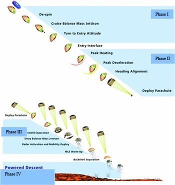
Figure 1. Sequence overview of recovering a payload from an orbit(1).
Pepper et al designed and developed the 24-foot diameter hybrid Kevlar-29/nylon ribbon parachute in 1980 and tested it with a sled test vehicle(Reference Pepper5). Kent developed a drag parachute for space shuttle orbiter and tested it in wind tunnel, the flight test of which was carried out in 2001(Reference Kent6). Heindel et al developed parachute tests for a missile descent system in 1999(Reference Heindel and Wolf7). Guidotti et al designed, developed, tested, and carried out in-flight qualification of a parachute recovery system in 2012(Reference Guidotti8). Gallon et al did verification and validation testing of the parachute decelerator system prior to the first supersonic flight dynamics test for the low density supersonic decelerator program in 2015(Reference Gallon and Witkowski9).
Kenig et al developed rigging test bed for validation of multi-stage decelerator extractions in 2013(Reference Kenig4). Lin designed and developed rocket-boosted test for testing a ribbon parachute in 1989(Reference Lin10). Machín et al advanced and tested the parachute system for the space station crew return vehicle in 2011(Reference Machín, Iacomini, Cerimele and Stein11). Braun et al successfully landed five robotic systems on the surface of Mars by supersonic parachute(Reference Braun and Manning12). Development of an interim parachute recovery system for a re-entry vehicle was done by Pepper in 1980(Reference Pepper13). Schatzle et al developed a vehicle with a two-stage parachute system in 1980(Reference Schatzle and Curry14). Design, fabrication, packing and testing of a cross-multistage parachute for ARIM-1 sounding was done by Thomas in 1999(Reference Thomas15). Thomas designed and developed the flight testing of a parachute orientation system to air-launch rockets into low earth orbit in 2007(Reference Thomas, Thomas and Morgan16).
Flight tests have advantages and disadvantages. Advantages include testing under real conditions, high reliability and integrated testing (the recovery system and other subsystems are tested at same time). On the other hand, this approach has some disadvantages such as high cost and time to test. This paper deals with the design and development of a Subsonic Tandem Deceleration System (STDS). STDS was designed at 0.8 Mach for a terminal payload descent rate of 10 m/sec, descending through an altitude of 10 k, with a 500 kg payload to be landed. In this study, for Verification and Validation (V&V) of STDS, flight test vehicles were designed and analysed. With regard to aforementioned four landing steps, the third step is illustrated in Fig. 1.
2.0 DEPLOYMENT SEQUENCE AND INFLATION
In expressing aerodynamic characteristics of a parachute, the terms ‘deployment’ and ‘inflation’ should be specifically defined. Deployment begins when the parachute is unpacked and finishes when suspension lines are exposed to initial stretch. This is a very complicated process due to unsteady and non-uniform air flow, the contrast between system aerodynamics with system dynamics, and the effects of the initial form of the canopy at the time of unpacking. Inflation begins after the suspension lines are stretched and fluid flows through the canopy; it continues until canopy reaches its final form. Although parachute inflation is as complex as its deployment, it is more important because when a parachute inflates at high speed, it creates a very large drag which causes the payload speed to plunge, so a large force is exerted on the parachute structure as a result. This force, known as initial impact, can damage parachute components or the descending payload.
Figure 2 shows stages of parachute inflation. It is evident that inflation begins with the suspension lines being stretched and the air flowing into the canopy. After parachute is deployed initially, a bulk of air moves through the canopy. As the bulk of air reaches the end of the canopy, superfluous air begins to flow into it. The parachute is initially inflated slowly, but as the entrance of the canopy begins to open, inflation is accelerated. Most of the seamless parachutes experience a surge in entrance pressure (over inflation) that makes the parachute shrink slightly.
Figure 2. Stages of parachute inflation(Reference Knacke21).
Moler and Shobel showed that a parachute is inflated at different speeds after a certain time period because the conical flow of air is constant toward the canopy, as shown in Fig. 3 (Reference Knacke21).
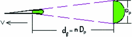
Figure 3. Conical flow of air toward the canopy(Reference Knacke21).
where Dp is the parachute diameter and df is the inflation time period. Because the diameter of the parachute varies at the time of inflation, the parachute's nominal diameter Do is used instead. Hence, assuming that parachute speed is not reduced during inflation, the following equation can be stated:
 $$\begin{equation}
{t_f} = \frac{{n{D_0}}}{{{V_0}}},
\end{equation}$$
$$\begin{equation}
{t_f} = \frac{{n{D_0}}}{{{V_0}}},
\end{equation}$$
where nis a constant and depends on the type of parachute. In practice, nominal diameter and speed reduction during inflation are considered in modeling, so the following relation is used:
 $$\begin{equation}
{t_f} = \frac{{n{D_0}}}{{{V^{0.9}}}}
\end{equation}$$
$$\begin{equation}
{t_f} = \frac{{n{D_0}}}{{{V^{0.9}}}}
\end{equation}$$
The drag area varies from 0% to 100% during inflation. This variation of area can be linear, nonlinear. Considering red reference(Reference Knacke21), variations of the drag area based at the time of inflation can be observed in Fig. 4.

Figure 4. Variations of drag area based on time of inflation for different parachutes(Reference Knacke21).
3.0 RECOVERY SYSTEM REQUIREMENTS
The design requirements for the recovery system are given below.
-
• All parachute packs must be cylindrical in shape.
-
• The 500 kg recovery system was not designed for a rate of descent at a specific sea level, but for a specified main parachute size.
-
• The four phases recovery system are designed in light of the payload weight, the maximum bearable acceleration of the assembly (10 g longitudinally and 3 g latitudinally), and the velocity of launching and landing.
-
• Total STDS weight added to the orbiter shall be less than 8 kg.
-
• STDS shall not impart any loads greater than 10 g longitudinally and 3 g latitudinally.
-
• STDS shall be capable of extraction from altitudes of 5,000-12,000 m.
-
• STDS total weight with payload shall be less than 500 kg.
To meet the scientific mission objective, the STDS had to be light in weight, packed into a small volume, and able to sustain the parachute opening loads. The drogue parachute had to quickly stabilise the payload from spinning, coning or tumbling. The main chute required a high drag coefficient for a slow payload descent.
Initial conditions such as altitude and velocity are provided by the aircraft.
4.0 RECOVERY SYSTEM DESIGN METHODOLOGY
The design of the recovery system was based on the past recovery systems. Design factors were determined for critical components following techniques in Knacke(Reference Knacke21). A margin-of-safety analysis is done on all critical components to ensure they meet design requirements. The design methodology is presented in Fig. 5; the number of recovery stages, parachute reefing and parachute size are determined according to this figure.
Figure 5. Design methodology.
4.1 Drogue systems
A conical ribbon parachute was selected for the drogue chute because it has high stability and load capabilities. A long Kevlar towline (or drogue riser) was needed to minimise the weight and meet the strength requirements to provide for stabilization of a flat spinning payload. The reefing delay was specified to be 10 seconds to allow use of the same reefing line cutters for all parachutes in the system. This helped to reduce inventory and cost during production. All material specifications were common, low-cost nylon materials.
4.2 Main parachute
A cross parachute was selected for the main parachute type. The 500 kg system was initially designed using a flat circular parachute. This system was redesigned to use a cross chute with considerable weight savings. The cross parachute has a relatively limited published history for recovery system use, compared to the more common circular parachute variations. Cross parachutes display a high level of stability around zero degree angle-of-attack. This high level of stability is a result of the high geometric porosity due to the “plus” shape construction. This porosity also helps in reducing the opening shock coefficient of the cross parachute, which is considerably below solid circular parachutes. A second advantage of the cross parachute is its relatively high drag coefficient.
Although the actual constructed diameter of a cross parachute needs to exceed a comparable drag flat circular parachute, the drag coefficient based on canopy area is very comparable to the flat circular parachute(Reference Knacke21). Drag coefficients in the range of 0.75 to 0.82 for cross parachutes.
The final major advantage of the cross parachute is the significant weight savings which is provided over a solid, circular parachute. In the redesign of the 500 kg, the reefing line length was determined assuming a flat circular curve to account for reduced effective fabric area in the lower portion of the cross parachute. of course, larger effective canopy area causes increasing reefing ratio and lead to increasing of the percentage(Reference Siewert, Seely, Smith, Silbert and Widows27).
5.0 RECOVERY SYSTEM DESIGN
In light of the payload weight, maximum bearable acceleration of the assembly (10 g longitudinally and 3 g latitudinally) as well as velocity of launching and landing, the three-phase recovery system is designed, To meet the science mission objective. The STDS had to be light in weight, packed into a small volume, and sustain the parachute opening loads. The drogue parachute had to quickly stabilise the payload from spinning, coning or tumbling. The main parachute required a high drag coefficient for a slow payload descent.
Mission parameters dictated a launch payload capable of lofting at 500 kg. The parachute is deployed at 0.8 Mach. Design challenges of the parachute recovery system were set by the scientific mission objective, for a terminal payload descent rate of 10 m/sec, descending through a 10 km altitude. The drogue parachute is a 20º conical continuous ribbon canopy with variable porosity and a 1.15 m nominal diameter. The suspension lines and radial members are Kevlar, while the ribbons are nylon of varying strengths. The main parachute is a cross with 10 m nominal diameter. For reducing acceleration on the payload, the main parachute has been reefed with a 2 m nominal diameter. The STDS Recovery System Configuration is shown in Fig. 6.
Figure 6. STDS recovery system configuration.
The STDS design and results are shown in Table 1.
Table 1 Characteristics of the recovery system

6.0 MISSION SCENARIO
Subsonic parachute tests are normally performed for re-entry payloads, particularly for space-related missions. Experimental setups for the chutes are usually planned for the wind tunnel or aboard an aircraft. However, a test projectile can also be employed for this purpose. For the latter case, a separate propulsion system is also needed to boost the parachute release system to supersonic speeds. Due to limitations of cost and time, a typical existing rocket system (RS) was utilised for this study. The RS is capable of accelerating the payload to a supersonic speed of M = 0.8(Reference Samani and Pourtakdoust17). The projectile had a diameter of 338 mm and is equipped with solid propellant. It was recovered by means of a set of main (reefing, full open) and drogue (conical loop-opening) parachutes. Based on the parachute's features and using flight simulation, a soaring height of l,700 m and a speed of l00 m/s were achieved. The projectile payload included a flight computer, navigation system, imager and image transmitter. The parachute ejects laterally out of its room. The flight computer is based on an AVR microcontroller that sends commands to the main and drag parachutes at certain times depending on the scenario. Noteworthy is that the system employs two IMUs.
7.0 MANUFACTURING, ASSEMBLING AND TESTING
Having completed the design process, subassemblies were manufactured and then tested. Testing was followed by an assembly process preceding flight testing that showed that the laterally separating systems, drag parachute, fully inflated main reef parachute, flight computer, telemetry system and imager were all functioning properly and the payload was safely recovered.
8.0 ROTATIONAL AND TRANSITIONAL MOTION EQUATIONS (FLIGHT SIMULATION)
The system was modeled through rotational and transitional motion equations in the body system. In relation to the transitional motion equations, there is:
 $$\begin{equation}
m\left[ {{{\dot{\vec{V}}}_m} + {\Xi _m}{{\vec{V}}_m}} \right] = {\vec{f}_a} + {\vec{f}_p} + m{T^{BG}}\vec{g}
\end{equation}$$
$$\begin{equation}
m\left[ {{{\dot{\vec{V}}}_m} + {\Xi _m}{{\vec{V}}_m}} \right] = {\vec{f}_a} + {\vec{f}_p} + m{T^{BG}}\vec{g}
\end{equation}$$
where m denotes mass, VI
m
is the velocity vector of phases in the body system, ∑m is the asymmetry matrix, ω
m
is the angular velocity of the projectile, fI
a
is the aerodynamic forces vector, fr
p
is the motor vector, TBG
G is the matrix of body system conversion into geographical system, and
 $\vec{g}$
is the vector of gravitational acceleration in geographical system(
Reference Roskam
18
,
Reference Blakelock
19
). Aerodynamic forces are as follows:
$\vec{g}$
is the vector of gravitational acceleration in geographical system(
Reference Roskam
18
,
Reference Blakelock
19
). Aerodynamic forces are as follows:
 $$\begin{equation}
{\vec{f}_a} = \left[ {\begin{array}{@{}*{1}{c}@{}} {{f_{{a_x}}}}\\ {{f_{{a_y}}}}\\ {{f_{{a_z}}}} \end{array}} \right]\, = q'\,S\left[ {\begin{array}{@{}*{1}{c}@{}} { - {c_A}}\\ {{c_Y}}\\ { - {c_N}} \end{array}} \right]\,\,,\,\,q' = \frac{1}{2}\rho \,{V_T}^2
\end{equation}$$
$$\begin{equation}
{\vec{f}_a} = \left[ {\begin{array}{@{}*{1}{c}@{}} {{f_{{a_x}}}}\\ {{f_{{a_y}}}}\\ {{f_{{a_z}}}} \end{array}} \right]\, = q'\,S\left[ {\begin{array}{@{}*{1}{c}@{}} { - {c_A}}\\ {{c_Y}}\\ { - {c_N}} \end{array}} \right]\,\,,\,\,q' = \frac{1}{2}\rho \,{V_T}^2
\end{equation}$$
In relation to the rotational motion equations, there is:
 $$\begin{equation}
\left[ {\frac{{d{\omega _m}}}{{dt}}} \right] = {[{I_m}]^{\, - 1}}\left( { - {\Xi _m}{I_m}{\omega _m} + {{\vec{m}}_{CG}}} \right)
\end{equation}$$
$$\begin{equation}
\left[ {\frac{{d{\omega _m}}}{{dt}}} \right] = {[{I_m}]^{\, - 1}}\left( { - {\Xi _m}{I_m}{\omega _m} + {{\vec{m}}_{CG}}} \right)
\end{equation}$$
where I m denotes matrix of mass inertial moment and mCG is the aerodynamic moment of the projectile, parachute and motor around the assembly centre of mass. Aerodynamic forces are as follows:
 $$\begin{equation}
{m_{{a_{CG}}}} = \left[ {\begin{array}{@{}*{1}{c}@{}} {{m_{{a_x}}}}\\ {{m_{{a_y}}}}\\ {{m_{{a_z}}}} \end{array}} \right]\, = q'\,SL\left[ {\begin{array}{@{}*{1}{c}@{}} {{c_L}}\\ {{c_m}}\\ {{c_n}} \end{array}} \right]\,
\end{equation}$$
$$\begin{equation}
{m_{{a_{CG}}}} = \left[ {\begin{array}{@{}*{1}{c}@{}} {{m_{{a_x}}}}\\ {{m_{{a_y}}}}\\ {{m_{{a_z}}}} \end{array}} \right]\, = q'\,SL\left[ {\begin{array}{@{}*{1}{c}@{}} {{c_L}}\\ {{c_m}}\\ {{c_n}} \end{array}} \right]\,
\end{equation}$$
All the aerodynamic factors are obtained from MD software(Reference Bruns, Moore, Stoy, Vukelich and Blake20). Parachute moments and forces are as follows:
 $$\begin{equation}
\begin{array}{@{}rcl@{}} {{\vec{f}}_p} &=& \frac{1}{2}\rho {V_m}^2{S_p}{C_D}_{_P}\\ \,\,{{\vec{m}}_p} &=& \vec{r} \times {{\vec{f}}_p}\, \end{array}
\end{equation}$$
$$\begin{equation}
\begin{array}{@{}rcl@{}} {{\vec{f}}_p} &=& \frac{1}{2}\rho {V_m}^2{S_p}{C_D}_{_P}\\ \,\,{{\vec{m}}_p} &=& \vec{r} \times {{\vec{f}}_p}\, \end{array}
\end{equation}$$
In addition, estimated drag surface in the parachutes' design is as follows( Reference Knacke 21 - Reference Lingard 26 ):
 $$\begin{equation}
\begin{array}{@{}rcl@{}} 20\, < t < 30\,\,,\,\,\,{S_p}{C_D}_{_P} &=& \,1.3\,\,{\rm{brake}}\,{\rm{parachute}}\\ 30\, < t < 40\,\,\,,\,\,\,{S_p}{C_D}_{_P} &=& \,12\,\,{\rm{main}}\,{\rm{parachute}}\,\,{\rm{in}}\,{\rm{reef}}\\ t > 40\,\,\,,\,\,\,{S_p}{C_D}_{_P} &=& 75\,\,\,{\rm{main}}\,\,{\rm{parachute}}\,\,{\rm{fully}}\,\,{\rm{deployed}}\,\,\, \end{array}
\end{equation}$$
$$\begin{equation}
\begin{array}{@{}rcl@{}} 20\, < t < 30\,\,,\,\,\,{S_p}{C_D}_{_P} &=& \,1.3\,\,{\rm{brake}}\,{\rm{parachute}}\\ 30\, < t < 40\,\,\,,\,\,\,{S_p}{C_D}_{_P} &=& \,12\,\,{\rm{main}}\,{\rm{parachute}}\,\,{\rm{in}}\,{\rm{reef}}\\ t > 40\,\,\,,\,\,\,{S_p}{C_D}_{_P} &=& 75\,\,\,{\rm{main}}\,\,{\rm{parachute}}\,\,{\rm{fully}}\,\,{\rm{deployed}}\,\,\, \end{array}
\end{equation}$$
The time required for the parachutes to fully inflate is obtained from Equation (2) where n denotes the inflation parameter, D is the parachute diameter and V is the flight speed. In order to obtain positions of the two phases in the inertial system, linear rotational kinematics are employed as follows:
 $$\begin{equation}
\left[ {\begin{array}{@{}*{1}{c}@{}} {\dot{x}}\\ {\dot{y}}\\ { - \dot{h}} \end{array}} \right] = {\bar{T}^{BG}}\left[ {\begin{array}{@{}*{1}{c}@{}} u\\ v\\ w \end{array}} \right]\,\,\,\,,\,\,\,\,\frac{{dz}}{{dt}} = - \frac{{dh}}{{dt}}
\end{equation}$$
$$\begin{equation}
\left[ {\begin{array}{@{}*{1}{c}@{}} {\dot{x}}\\ {\dot{y}}\\ { - \dot{h}} \end{array}} \right] = {\bar{T}^{BG}}\left[ {\begin{array}{@{}*{1}{c}@{}} u\\ v\\ w \end{array}} \right]\,\,\,\,,\,\,\,\,\frac{{dz}}{{dt}} = - \frac{{dh}}{{dt}}
\end{equation}$$
Furthermore, to obtain rotational kinematics, quaternion relations whose differential equations are as follows are used.
 $$\begin{equation}
\hspace*{-10pt}\left\{ {\dot{q}} \right\} = \frac{1}{2}\left\{ {\begin{array}{@{}*{4}{c}@{}} 0&{ - p}&{ - q}&{ - r}\\ p&0&r&{ - q}\\ q&{ - r}&0&p\\ r&q&{ - p}&0 \end{array}} \right\}\left\{ {\vec{q}} \right\}\,\,,\,\,\left\{ {\vec{q}} \right\}\, = \left\{ {\begin{array}{@{}*{1}{c}@{}} {{q_0}}\\ {{q_1}}\\ {{q_2}}\\ {{q_3}} \end{array}} \right\}\begin{array}{@{}*{2}{c}@{}} ,\quad\qquad&\begin{array}{@{}l@{}} \tan \phi = \displaystyle\frac{{2({q_2}{q_3} + {q_0}{q_1})}}{{{q_0}^2 - {q_1}^2 - {q_2}^2 - {q_3}^2}}\\[8pt] \sin \theta = - 2({q_1}{q_3} - {q_0}{q_2})\\[6pt] \tan \psi = \displaystyle\frac{{2({q_1}{q_2} + {q_0}{q_3})}}{{{q_0}^2 + {q_1}^2 - {q_2}^2 - {q_3}^2}} \end{array} \end{array}\quad
\end{equation}$$
$$\begin{equation}
\hspace*{-10pt}\left\{ {\dot{q}} \right\} = \frac{1}{2}\left\{ {\begin{array}{@{}*{4}{c}@{}} 0&{ - p}&{ - q}&{ - r}\\ p&0&r&{ - q}\\ q&{ - r}&0&p\\ r&q&{ - p}&0 \end{array}} \right\}\left\{ {\vec{q}} \right\}\,\,,\,\,\left\{ {\vec{q}} \right\}\, = \left\{ {\begin{array}{@{}*{1}{c}@{}} {{q_0}}\\ {{q_1}}\\ {{q_2}}\\ {{q_3}} \end{array}} \right\}\begin{array}{@{}*{2}{c}@{}} ,\quad\qquad&\begin{array}{@{}l@{}} \tan \phi = \displaystyle\frac{{2({q_2}{q_3} + {q_0}{q_1})}}{{{q_0}^2 - {q_1}^2 - {q_2}^2 - {q_3}^2}}\\[8pt] \sin \theta = - 2({q_1}{q_3} - {q_0}{q_2})\\[6pt] \tan \psi = \displaystyle\frac{{2({q_1}{q_2} + {q_0}{q_3})}}{{{q_0}^2 + {q_1}^2 - {q_2}^2 - {q_3}^2}} \end{array} \end{array}\quad
\end{equation}$$
Results from Section 4 (characteristics of the recovery system such as performance time of each parachute and recovery altitude), and Section 5 (the mission scenario is presented in Fig. 7) are used in the equations above. To validate the recovery design, results of the simulations are compared with final velocity and the maximum acceleration of each parachute, which are determined in Table 1.
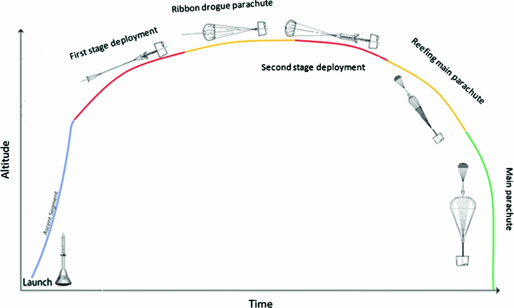
Figure 7. Testing mission scenario.
9.0 RESULTS AND DISCUSSION
Figures 8 and 9 show results of the imaging system. As Fig. 10 shows, the maximum acceleration equal to 10 g is obtained at t = 2.9 during the flight. This acceleration value is within the permissible limits of the design. Figure 11 shows that at the beginning of the deployment at t = 20, drag parachute starts functioning, with the result that a negative axial acceleration is exerted on the system because the parachute is located near the nose. A moment is immediately produced around the system centre of mass by the parachute which leads to inverse acceleration; the value of acceleration changes from ax = –2.8 g to ax = 3.8 g. Then at t = 31.15 the main parachute functions in the reef phase followed by the start of the major phase of the main parachute at t = 40. As it can be seen in the Fig. 11, drag coefficients of the reef phase have been precisely estimated; while coefficients of the drag parachute and major phase of the main parachute see a deviation of 18% and 37% respectively, which will be corrected. As Fig. 12 shows, the test range Rtest = 2,568 m is obtained, while Rsim =2,525 m. So a deviation of 1.67% is present over the range. Figure 13 indicates the velocity over time until the payload has touched down at the safe speed of 9 m/sec.
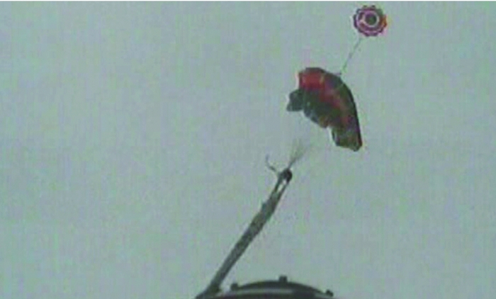
Figure 8. Initial inflation of the main parachute.
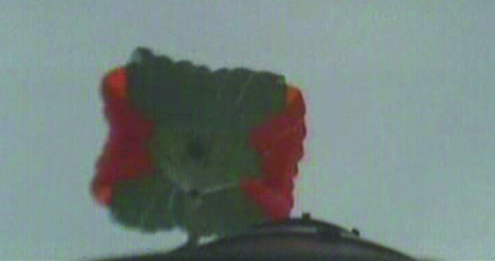
Figure 9. lnflated main parachute at the end of reef phase.
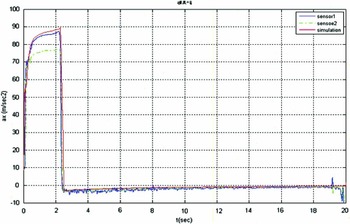
Figure 10. Axial acceleration (simulation and test) by time.
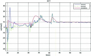
Figure 11. Parachute axial acceleration (simulation and test) over time.

Figure 12. Height by range.

Figure 13. Deceleration over time.
10.0 CONCLUSIONS
This paper deals with design and development of an STDS system. It includes a conical drogue parachute and cross parachute as the main parachutes, which reef for 10 seconds. A cross parachute provided the low cost and relatively easy fabrication characteristics along with the high drag, high stability and low weight parameters needed to meet all aspects of the design concerns. To decrease weight and cost, the main parachute is reefed. A thorough analysis has been done on the systems to ensure that performance will meet the recovery system specifications. The STDS system has reduced system cost and required testing while increasing reliability and conformance to specifications. The flight system has demonstrated the useful advantages of cross parachutes and production considerations in recovery system applications. As seen in Fig. 10, maximum acceleration is verified at 10 g at t = 2.9 of the flight, which is within the permissible limits of the design.
Figure 11 shows the deployment of drogue parachute at t = 20, according to this data the value of acceleration changes from ax = –2.8 g to ax = 3.8 g which related to deployment parachute and velocity Decelerator. Then at time t = 31.15 the main parachute is deployed in the reef phase for 10 sec. The main parachute was deployed at t = 41.15. As it can be seen in the Fig. 11, drag coefficients of the reef phase have been precisely estimated; while coefficients of the drag parachute and the major phase of the main parachute sees a deviation of 18% and 37% respectively, which will be corrected. According to Fig. 12, Rang-test and Rang-sim have deviations of 1.67%. Figure 13 indicates the velocity per time when the payload has touched down at the safe speed of 9 m/sec. This paper offers a four-phase scenario for recovering a space payload and tests the fourth phase. Design, manufacture and test procedures are then studied for the payload recovery at subsonic speeds. The recovery process is carried out by means of a drag parachute and a main parachute. Conformity of the simulation results and sensors outputs plus the results obtained from CCD imagers show that the test is completely successful and system design requirements are fulfilled.


