


Nomenclature
- a
-
actions selected according to the policy at current state s
- r
-
reward
- s
-
current observation states
- s’
-
next states after actions
- Q(s, a)
-
Q-value function: Critic for select action a at state s
- R(s, a)
-
reward function: reward for choosing action a at state s
- P(s’|s,a)
-
probability function: tendency to select action a at state s to get s’
- J
-
objective function
- L
-
loss function
- N
-
minibatch size
- π
-
reinforcement learning policy
- θ
-
policy parameters
- θ μ
-
Actor function distribution parameters
- θ Q
-
Critic function distribution parameters
- μ
-
Actor function distribution
- Q
-
Critic function distribution
- γ
-
reward decay coefficient
- α
-
learning rate
- τ
-
target update factor
- N t
-
random process noise
1.0 Introduction
In the United States, Russia and other western developed countries, the use of unmanned aerial vehicles (UAVs) in the battlefield for reconnaissance, interference and strike missions has become the norm. In recent years, with the continuous development of artificial intelligence technology, the combat mode of UAV has gradually developed from ‘single combat’ to ‘cluster intelligence’, and has become a key research topic in the military field of various countries [Reference Xing, Zhen and Gong1–Reference Wu, Yu and Li5].
UAV cluster combat generally refers to the simultaneous deployment of hundreds of small, fast and high-performance UAVs in the battlefield airspace. UAVs build bionic formations by simulating the clustering behaviour of swarms, schools of fish and ant colonies, carry out interactive communication through various channels, such as combat data link system, tactical radio system and communication relay network, and finally realise operational coordination based on cloud computing, big data and artificial intelligence and other advanced technologies. UAV cluster can carry out strategic deterrence, campaign confrontation and tactical operations in military operations and make the capability of a single UAV be expanded and the overall combat effectiveness of the multi-UAV system can be improved [Reference Dong, Ai and Liu6–Reference Xu, Long and Wang8]. With the continuous integration and development of unmanned systems and intelligent technologies, the actual combat degree of UAV cluster warfare is constantly improving, and it is gradually stepping into the battlefield and opening the curtain of intelligent warfare. In 2015, the US Naval Research Office announced the LOCUST program. Next, DARPA issued the Gremlins program. Unmanned aerial vehicles (UAVs) with electronic payloads and collaboration capabilities are launched outside the defensive area for offshore reconnaissance and electronic attacks. In 2017, the US Perdix micro-UAV high-speed launch demonstration project made a new breakthrough. The successful launch of 103 micro-UAVs from three F/A-18F fighters at Mach 0.6 demonstrated advanced group behaviour and mutual coordination ability. Following, China has again set a world record for swarm flights of fixed-wing UAVs. One hundred nineteen fixed-wing drones successfully demonstrated the actions such as dense catapult take-off, aerial assembly, multi-target grouping, formation and encirclement. But these research achievements just stay at the cluster operation concept demonstration stage and fail to realise the autonomous decision and intelligent control. Considering that the future battlefield will have higher and higher requirements for real-time and intelligence, it is very important to truly realise autonomous and intelligent cooperative operation of UAV cluster by studying the application of intelligent control algorithm in different cluster combat tasks, for seizing the initiative of future air combat [Reference Zhao, Chao and Wang9–Reference Fu, Pan and Wang17].
UAV cluster as a Multi-Agent System (MAS) [Reference La, Nguyen and Le18–Reference Busoniu, Babuska, Schutter, Srinivasan and Jain21], the environment model and dynamic model are both complex. Each agent in the cluster needs to consider the influence from the actions of other agents, and the dynamics of the environment when learning behaviour strategies. However, traditional Reinforcement Learning (RL) [Reference Musavi, Onural and Gunes22–Reference Silver, Lever and Heess30] algorithms are mainly for a single agent, so they are not applicable for cluster control. For Deep Q-Network (DQN) [Reference Mnih, Kavukcuoglu and Silver26,Reference Duryea, Ganger and Hu31] algorithm based on Q-learning [Reference Littman32,Reference Gong, Wang and Hu33], a single agent in MAS will be affected by the state of other agents, resulting in different state transitions and making the method of experience replay no longer applicable. For Policy Gradient (PG) [Reference Yang and Wei29,Reference Peters and Schaal34] method, the continuous changes in the environment and the increase in the number of agents will lead the learning variance to increase further. Therefore, we propose to use Multi-Agent Reinforcement Learning (MARL) [Reference Babuska, Busoniu and Schutter35–Reference Guo and Meng39] algorithm to realise the cooperative control of UAV cluster.
The research on the intelligent collaborative control of UAV cluster is mainly to construct efficient learning framework and rigorous reward mechanism. Considering the instability of the environment in MAS and the interaction among agents, and refering to the Lowe’s research [Reference Lowe, Wu and Tamar40], we made some key improvements on the basis of the weaknesses of the original Multi-Agent Deep Deterministic Policy Gradient (MADDPG) algorithm. The improved new learning framework and more strict reward mechanism both make the algorithm be able to obtain more accurate evaluation values, making the learned behaviour strategy more optimised. Successfully realise the autonomous cooperative control of UAV cluster.
The paper is organised as follows. Section 2 introduces the background and development of the Reinforcement Learning algorithms. Section 3 explains in detail the improved MADDPG algorithm and the reasons for improvement. Section 4 shows the experimental setup of two conventional combat missions for UAV cluster. Section 5 shows the simulation results of the improved MADDPG algorithm on two conventional combat missions, and the comparison with the MADDPG before improved. The conclusions and future work are presented in Section 6.
2.0 Background
RL is an online learning technique that is different from supervised and unsupervised learning methods. It regards learning as a process of attempt and evaluation. First, the reinforcement learning system perceives the state of the environment and then takes a certain action and act on the environment. After the environment accepts the action, the environment state changes and gives a reinforcement signal (reward or punishment) at the same time as the feedback to the reinforcement learning system. The reinforcement learning system selects the next action based on the reinforcement signal and current state of the environment. The principle of the selection is to increase the probability of being rewarded. The selected action not only affects the state of the environment at the next moment, but also the final reinforcement value. The agent in reinforcement learning system can continuously accumulate experience just by many times’ attempts, and finally get the best behaviour strategy [Reference Wu, Yu and Li5,Reference Mnih, Kavukcuoglu and Silver26–Reference Silver, Lever and Heess30]. Traditional RL algorithms are mainly for the single agent system (SAS), so later we also call them Single-Agent Reinforcement Learning (SARL) algorithm. Traditional RL algorithms can be divided into value-based reinforcement learning, the reinforcement learning based on policy gradients and Actor-Critic network.
As the most basic value-based reinforcement learning algorithm, Q-Learning algorithm [Reference Duryea, Ganger and Hu31,Reference Gong, Wang and Hu33] is used to guide the agent’s actions by calculating the Q-value of each state and action pair and storing it in Q-table. But this algorithm is only applicable to the environment where the state space and the action space are both small and discrete. In actual control model, state space and action space are large. If the Q-table is used to record the state and action pair of each computation, the table will be very large. It will cost much time when inquiring about the maximum Q-value. In order to solve the problem that the state and action space in real control model are too large to lookup in Q-table, it is proposed to use Deep Neural Network (DNN) to predict the Q-value and learn the optimal strategy. The reason is that DNN has a good effect on the extraction of complex features. Therefore, Deep Q-Network (DQN) [Reference Mnih, Kavukcuoglu and Silver26] combining deep neural network and Q-Learning algorithm was proposed. It is a model-free deep reinforcement learning algorithm and has three key technical improvements: The first one is to approximate the value function using deep convolutional neural network; the second one is using the target network to update the target Q-value to ensure parameter convergence; and the third one is to use an experience replay buffer to store the labeled data samples, which can break the correlation of random sampling in neural network and improve the update efficiency. Although the DQN algorithm has been able to solve the problem of high-dimensional state or action space, this value-based reinforcement learning algorithm is only applicable to discrete space. It has insufficient processing capacity for high-dimensional continuous space and cannot solve the problem of random strategy. Therefore, the reinforcement learning algorithm based on policy gradient was proposed as another kind of RL algorithm.
Policy Gradient (PG) [Reference Yang and Wei29] algorithm omits the intermediate steps and directly selects actions based on the current state. It can enhance and weaken the possibility of choosing actions by computing reward, so there is no need to compute Q-values. For good behaviours, it will increase the probability being selected next time, and for the bad ones, the probability being selected next time will be weakened. After the random strategy is obtained through PG learning, the optimal strategy probability distribution needs to be sampled at each step of the behaviour selection to obtain the specific value of the action. The action space is usually high-dimensional, so there is no doubt that frequent sampling is a waste of computing power. Besides, the strategy usually converges to a local optimal rather than a global optimal. For the action space, it may be continuous values or very high-dimensional discrete values, so that the spatial dimension of the action is extremely large. If we use a stochastic strategy, we need to study the probabilities of all possible actions, and the number of samples required is very large. So the deterministic strategy is came up with to simplify the problem. It makes the determined value of the action at each step can be obtained directly by calculating the selected action. It is Deterministic Policy Gradient (DPG) [Reference Silver, Lever and Heess30] algorithm.
Combining the value-based reinforcement learning method and the reinforcement learning method based on policy gradient, a new algorithm called Actor-Critic (AC) [Reference Lillicrap, Hunt and Pritzel41–Reference Baker, Gupta and Naik44] network is generated. It can not only select the appropriate action in the continuous action space, but also evaluate the selected action by calculating the reward. For AC algorithm, the model involves two neural networks: Actor network and Critic network. Actor network has the same function with PG algorithm, which is responsible for generating actions and interacting with the environment. It selects the appropriate actions in the continuous action space with policy functions and round update, so the learning efficiency is relatively slow. Critic network apply a value-based algorithm to achieve single-step update, such as Q-Learning. The value function in algorithm is responsible for evaluating the selected actions and directing the next actions. Each time a parameters update is performed in a continuous space, and there is a correlation between the parameters before and after updating. That is to say, the training data of the model is no longer an independent and identical distribution, which leads the neural network to take a one-sided view of the problem.
In order to solve the above problems, an improved reinforcement learning algorithm called Deep Deterministic Policy Gradient (DDPG) [Reference Liu, Liu and Cai45–Reference Xu, Hui and Liu48] was proposed. It not only draws on the key technologies of the experience replay mechanism and target network from DQN, but also solves the problem of difficult convergence. DDPG adopts Convolutional Neural Network (CNN) as the simulation of policy function
 $\mu $
and
$\mu $
and
 ${Q^\mu }$
. The paramater
${Q^\mu }$
. The paramater
 $\mu $
comes from the policy network and
$\mu $
comes from the policy network and
 ${Q^\mu }$
is the parameter of Q network. The roles of these two networks are similar to Actor and Critic networks, respectively. We update Q-value by minimising the loss function:
${Q^\mu }$
is the parameter of Q network. The roles of these two networks are similar to Actor and Critic networks, respectively. We update Q-value by minimising the loss function:
 \begin{equation} L = \frac{1}{N}{\sum\nolimits_i {\left[ {{r_i} + \gamma {Q^\prime}({s_{i + 1}},{\mu ^\prime}({s_{i + 1}}|{\theta ^{{\mu ^\prime}}})|{\theta ^{{Q^\prime}}}) - Q({s_i},{a_i}|{\theta ^Q})} \right]} ^2}\end{equation}
And use the sampled gradient to update the policy:
 \begin{equation}{\nabla _{{\theta ^\mu }\mu {\rm{|}}{s_i}}} \approx \frac{1}{N}\sum\limits_i {{\nabla _a}Q(s,a|{\theta ^Q}){|_{s = {s_i},a = \mu ({s_i})}}{\nabla _{{\theta ^\mu }}}} \mu (s|{\theta ^\mu })|{s_i}\end{equation}
The target networks adopted in DDPG are updated by
 ${\theta ^{{Q^\prime}}} \leftarrow \tau {\theta ^Q} + (1 - \tau ){\theta ^{{Q^\prime}}}$
and
${\theta ^{{Q^\prime}}} \leftarrow \tau {\theta ^Q} + (1 - \tau ){\theta ^{{Q^\prime}}}$
and
 ${\theta ^{{\mu ^\prime}}} \leftarrow \tau {\theta ^\mu } + (1 - \tau ){\theta ^{{\mu ^\prime}}}$
. One advantage of DDPG algorithm is that it can use only low-dimensional observations to learn competitive policies. And another advantage is that it can do off-policy exploration. For continuous action space, DDPG algorithm converges faster than DQN algorithm.
${\theta ^{{\mu ^\prime}}} \leftarrow \tau {\theta ^\mu } + (1 - \tau ){\theta ^{{\mu ^\prime}}}$
. One advantage of DDPG algorithm is that it can use only low-dimensional observations to learn competitive policies. And another advantage is that it can do off-policy exploration. For continuous action space, DDPG algorithm converges faster than DQN algorithm.
In recent years, with the introduction of the concept of cluster, the emphasis of reinforcement learning has gradually shifted to MARL. MARL means that multiple agents in cluster interact with the environment through ‘trial and error’, and each agent has an impact on the environment. The agents in cluster have complex relationships, and their interests may be aligned, not entirely aligned, or completely opposite. And the cluster can be cooperative, competitive, or both. In MAS, each agent needs to learn its own optimal strategy to maximise its utility. The environment of SAS is stable, but in MAS, each agent constantly learns and improves its strategy by interacting with the environment and calculating the reward value. Therefore, from the perspective of each agent, the environment is complex and dynamically unstable, which no longer meets the convergence conditions of traditional reinforcement learning algorithms. It is precisely because of the instability of MAS environment that the behaviour strategies of each agent will not be completely consistent. In MAS, the behaviour of any agent will affect the system environment and the behaviour choices of other agents. When one agent’s strategy changes, other agent’s optimal strategy may also change, which will affect the convergence of the algorithm and make the design of the reward function more complicated. For DQN algorithm, the agent’s own state transfer will be different under the influence of other agents’ states, resulting in the experience replay method is no longer applicable. For PG algorithm, the constant change of environment and the increase of agent number will lead to the further increase of learning variance. At the same time, the dimensions of the connected actions combined by the current actions of each agent will also increase exponentially with the increase of the number of agents. As a result, strategy learning becomes complex and time consuming. Comprehensively considering the above difficulties, after getting familiar with the SARL algorithm, especially the implementation principle of DDPG algorithm, Multi-Agent Deep Deterministic Policy Gradient (MADDPG) algorithm [Reference Lowe, Wu and Tamar40] is proposed. It is a MARL algorithm combining AC network and DQN algorithm, and has the following three characteristics: (1) The optimal strategy obtained after learning can output the optimal actions using only local information; (2) No need to obtain the dynamic model of the environment in advance; (3) Not only suitable for cooperative environment, but also suitable for competitive environment.
3.0 Methods
Although he MADDPG algorithm adopted in Ref. [Reference Lowe, Wu and Tamar40] has been able to solve the problem of collaboration among multiple agents, there are still serious problems such as low learning efficiency, long time consuming and many internal collisions when testing in the simulation scene set in Section 4 of this paper. Therefore, we made key improvements to the learning network framework and the setting of reward function on the original algorithm in view of these deficiencies, and demonstrated the superiority of the improved algorithm through simulation comparison.
Improved MADDPG algorithm is similar to the original MADDPG algorithm in principle. It’s essentially an Actor-Critic network, but makes a series of improvements to the Actor-Critic algorithm. These improvements makes a new algorithm more suitable for complex multi-agent scenarios. First, the improved MADDPG algorithm adopts the strategy of centralised training with decentralised execution. During training, the Critic network and Actor network are trained using centralised learning. Actor network selects an action to execute according to the current state. The Q-value of the current state-action pair is calculated by the Critic network and fed back to the Actor network. Critic network trains based on the estimated Q-value and the actual Q-value, and Actor network updates its strategy based on the feedback. In the test phase, you only need the Actor network to make actions and no longer need the feedback from the Critic network. Therefore, during training, we can add some additional information to the Critic network to get a more accurate Q-value, such as the states and actions of other agents. That is the meaning of concentrated training. Agent evaluates the current action not only according to its own situation, but also the information of other agents. The decentralised execution means that after each agent is fully trained, the agent can quickly complete the selection of the optimal action only according to its own state and no longer needs the states and actions of other agents. It can greatly reduce the amount of data required for calculation. Second, the improved MADDPG algorithm also adjusts the observation data recorded in the experience replay buffer. We change the state and action of a single agent to the joint state and action of all agents. And we also use the strategy set effect optimisation method to make each agent learn their own different strategies, and finally use the overall effect of all strategies to determine the optimal strategy. The main purpose of this improvement is to improve the stability and robustness of MADDPG algorithm. Actually, the improved MADDPG algorithm is essentially also a DPG algorithm. For each agent, a Critic network requiring global information and an Actor network needing local information can be obtianed through training, and each agent has its own reward function. So, the new improved MADDPG algorithm can be used not only for cooperative tasks but also for adversarial tasks, and the action space can also be continuous.
The structure of the improved MADDPG algorithm mainly includes Q network and P network, as shown in Fig. 1, and these two networks are trained at the same time. The function of Q network is consistent with the function of DQN algorithm. The difference is that the input data is expanded to the states and actions of all agents in the MAS environment. Therefore, it can be considered that Q network is the overall evaluation of cluster behaviour. However, P network is to conduct behaviour selection and optimisation learning for a single agent in the cluster. The first half of P network computes a probability distribution of all possible actions for the agent’s current state, which is equivalent to Actor network. The latter part works like a Critic network. Since the change of the behaviour of a single agent in the cluster will lead to the instability of the whole system, the states and actions of other agents must be taken into account when evaluating the behaviour of this agent. The final training results are the output of the optimal actions. For the improved algorithm, the innovation of the network structure is that the structure of P network is different from that of traditional Actor-Critic network. It treats the Actor network and Critic network as a whole for training and determines the optimal action by maximising the Q-value.

Figure 1. MADDPG algorithm structure. (a) Q network, and (b) P network.
The specific structure of the improved P network is shown in Fig. 2. By comprehensively considering the state variables and action variables of all agents, the calculated Q-value is more accurate and the behaviour selection is more optimised.

Figure 2. Improved P network framework.
The specific steps of the improved MADDPG algorithm can refer to the followings:

4.0 Mission Scenarios
The improved MADDPG algorithm is used to construct a multi-agent reinforcement learning model for two conventional combat missions: navigation and location regional reconnaissance and round-up confrontation. After the task instruction is determined, the cluster can use the corresponding reinforcement learning model to learn autonomously and complete the selection of the optimal strategy, so as to achieve multiple UAVs’ task distribution and formation cooperative control, and finally complete the target task quickly and efficiently.
4.1 Regional reconnaissance
Regional reconnaissance can be divided into two parts: The first part is to complete location determination, and the second is to navigate to the corresponding coordinate points. Location determination requires the UAV cluster to independently complete the location distribution according to the number of cluster and the area to be detected. At the same time, it requires to ensure that the cluster can cover the largest area without missing any information. According to the detection perspective of each UAV, the reinforcement learning algorithm is used to perform autonomous calculations to achieve cluster allocation and formation control [Reference La49,Reference La, Sheng and Chen50]. Because UAVs with the same detection angle have different detection areas at different heights, the higher the height, the larger the area, the more information, but the details are not clear enough. In order to ensure the full coverage of the area when the number of clusters is determined, the algorithm should be able to quickly calculate according to the area to be investigated, and independently complete the optimal allocation of each UAV in the cluster. The detailed implementation method can refer to the Refs [Reference Adepegba, Miah and Spinello51] and [Reference Pham, La and Feil-Seifer52]. The second part is to make the UAV cluster to formulate optimal navigation schemes based on recent principles by observing the relative position of each UAV. The goal is to make the corresponding UAVs be able to reach the designated location as soon as possible without internal collisions. The specific implementation plan can refer to Fig. 3.

Figure 3. Cooperative navigation.
In this paper, we mainly study how the UAVs in cluster can complete mission assignment and reach the corresponding positions through cooperative communication without internal collisions. We call it cooperative navigation in later study.
In the environment of cooperative navigation, N UAVs must cooperate through physical actions to reach a set of N landmarks. Each UAV makes the task arrangement by observing the relative positions of other UAVs and all the landmarks and considering all UAVs’ distances from arbitrary landmarks. In other words, the UAV cluster has to cover all of the landmarks using the least time. Further, these UAVs will be penalised when colliding with each other. The goal of cooperative navigation is to enable the cluster to assign targets autonomously and enable UAVs to reach the corresponding location as quickly as possible without colliding with each other.
4.2 Round-up confrontation
When carrying out tracking, encircling, and enemy-to-self confrontation, we must first complete the assignment of mulitple targets. That is assigning different targets to the corresponding UAVs to simultaneously complete multiple targets’ tracking and striking. Typically, it is the least expensive arrangement to allocate three UAVs round up a target. The specific scheme design can refer to Fig. 4. It shows the combat plan that multiple UAVs cooperate to round up and attact one target. And the attaction mode adopts the suicidal destruction combat mode. It means that arranging any one UAV to hit the target. It requires that several UAVs with the same combat target and combat mission can communicate with each other and cooperate to complete the target mission while avoiding internal collisions. This is a problem of cooperative control in the MAS, so we plan to use MARL algorithms to complete the autonomous perception and learning of multiple agents in order to obtain the optimal cooperation strategy.

Figure 4. Cooperative round-up confrontation.
In the environment of round-up confrontation, N slower cooperative UAVs must chase a faster target UAV around a randomly generated environment with L large obstacles impeding the way. One UAV chooses actions by observing the relative positions and velocities of the other UAVs, and the positions of the obstacles. Each time any one UAV in the cluster collides with the target UAV, the cluster will be rewarded while the target UAV is penalised. If there is one collision in cluster, the cluster will receive one punishment. The more collisions, the more punishments. In addition, when the cluster don’t capture the target, the reward function of cluster is related to the relative distance between the target UAV and each UAV in cluster. The reward value will decrease as the distance from the target increases. To the contrary, the target’s reward will increase with the distance increasing.
5.0 Simulation Results
5.1 Simulation tests on cooperative navigation
We compiled the environmental document of cooperative navigation mission and constructed the learning framework of the improved MADDPG algorithm. In the environmental document, we assigned three UAVs to reach three designated locations in the shortest possible time and made sure these UAVs didn’t collide with each other. When we set up the algorithm network, we designed Q network and P network separately. Wherein, the structure of Q network and P network are similar to the structure of Actor-Critic network. It uses a fully connected neural network with two hidden layers, shown in Fig. 2. The number of nodes of each layer is 128. In both hidden layers, the activation functions are rectified linear units (Relu) functions. In order to make the choice of action more optimised and the evaluation of action more accurate, the tangent hyperbolic (tanh) function is applied in the output layer of the Actor network, and the action variables output by the Actor network are introduced in the input layer of the Critic network. These changes are the improvements for the original algorithm, which can increase the learning efficiency and optimise the learned policy.
Besides, we also improved the reward mechanisms because policy learning is based on reward values. The states available to the algorithm are the current position of each agent and the location of each landmark. To compile simply, we test the improved MADDPG algorithm in two-dimensional environment, and make the agents do uniform motion. We initialise the initial coordinate position of each agent and the specified target positions, respectively, making coordinates x and y to be any value in the range of −1 to 1, respectively. The reward value for each agent is initialised to 0 before the iteration training begins. During training, the UAVs in the cluster select actions randomly and compute the rewards according to the reward mechanisms, then evaluate the current actions to optimise the action selection. After several iterations, the optimal policy can be obtained. At this point, UAV cluster can autonomously select actions according to the optimal policy to carry out the cooperative navigation task as soon as possible.
The reward function of each UAV is calculated with its actual position and the designated locations. Because the UAV cluster is fully cooperative relationship in cooperative navigation mission, we must consider the whole cluster when calculating the reward value. That is to consider all the distances from each UAV to each landmark. Since the algorithm must first ensure that each landmark must have one UAV to reach, we hope that the UAVs can complete collaborative allocation and adjust the scheme at any time as the situation changes, so that the nearest UAV to the landmark to cover. Therefore, when the reward function is set, the reward value should increase as the relative distance between the UAV and the landmark decreases. To achieve collaborative allocation and avoid multiple UAVs covering the same landmark, we need to add collision avoidance settings. When two UAVs have the same distance from the same landmark and are both closest, they can coordinate one of them to the second nearest landmark according to the principle of avoiding collision, eventually realising the full coverage of all landmarks. Since it is a problem of full cooperation, we need to calculate the total reward value of the whole cluster under the current actions and learn the policy accordingly. For one agent (the agent in the text is UAV), we calculate the distances of all landmarks to it and take the minimum distance to compute the reward. In order to occupy the designated locations, the agent’s reward has a negative correlation with the minimum distance. The shorter the distance, the closer to the landmark, the larger the reward. Considering the size of agents and landmarks, we think the agent occupys the landmark when the distance is less than the sum of their radii (the sum is 0.1). As a reward, we make the reward value add 10. So the reward function of each agent is made as the following equation.
 \begin{equation}reward = \left\{ {\begin{array}{*{20}{c}}{\begin{array}{*{20}{c}}{reward - 0.1 \times \min (dists)} ,\quad {\begin{array}{*{20}{c}}{if} {\ \min (dists)}\end{array}}\end{array} \ge 0.1}\\{\begin{array}{*{20}{l}}{reward{\rm{ + }}10 \begin{array}{*{20}{c}},\qquad\qquad {\begin{array}{*{20}{c}}{} {}\end{array}} {}\end{array}} {else}\qquad\quad {\begin{array}{*{20}{c}}{\begin{array}{*{20}{c}}{\begin{array}{*{20}{c}}{} {}\end{array}} {}\end{array}} {}\end{array}}\end{array}}\end{array}} \right.\end{equation}
 \begin{equation} dists = {\left| {{s_{agent}} - {s_{landmar{k_i}}}} \right|_{i = 1, \cdots ,n}}\end{equation}
Wherein,
 ${s_{agent}}$
refers to the position of an agent waiting to be calculated the reward, and
${s_{agent}}$
refers to the position of an agent waiting to be calculated the reward, and
 ${s_{landmark}}$
is the position of any one designated locations. In order to avoid internal collision in the process and multiple agents covering the same landmark, we make the following settings. If one agent collides with another one, the agent should be punished, and the reward should be subtracted 10 for one collision. The total reward value per episode of the cluster are shown in Fig. 5.
${s_{landmark}}$
is the position of any one designated locations. In order to avoid internal collision in the process and multiple agents covering the same landmark, we make the following settings. If one agent collides with another one, the agent should be punished, and the reward should be subtracted 10 for one collision. The total reward value per episode of the cluster are shown in Fig. 5.

Figure 5. The total reward per episode for the cluster.
In Fig. 5, the total reward generally increases with episodes. During the first 10,000 episodes, it is a tentative learning phase, the cluster is exploring the rules through trial and error. At the same time, we also add disturbances to increase the uncertainty of the environment. So the reward value is decreasing fast. But in the next episodes, the reward continues to increase rapidly. It indicates that the cluster learns and trains through the improved MADDPG algorithm and the learning efficiency is high. According to the reward mechanism we set, if the UAV cluster could cover all landmarks, the reward value should be close to 30. From Fig. 5, it’s clear that the total reward value of cluster can reach 30 near to 60,000 episodes, which indicates that the three UAVs can cover three different landmarks without internal collisions.
To better observe the simulation results, we output a frame of image every 30,000 time steps to display the training process in an animated manner. Figure 6 shows the training results under two scenarios chosen from 60,000 scenarios. Figure 6(a) is the common case where the assigned landmarks are dispersed. In this case, the cooperative navigation mission is completed when the UAV cluster can cover or approach all the designated landmarks separately. Figure 6(b) shows a special case where two designated landmarks are very close. Under this circumstance, the policy learned through the improved MADDPG algorithm will automatically arrange a nearest UAV to cover the two landmarks at the same time. It can avoid damage caused by collision between UAVs.

Figure 6. The training process for cooperative navigation. (a) The common scenario where the assigned landmarks are dispersed, and (b) the special scenario where two designated landmarks are very close.
5.2 Simulation tests on round-up confrontation
In the environmental document of round-up confrontation, we depart the agents into good agents and adversary agents, and command adversaries to chase and attack good agents. The states available to the improved MADDPG algorithm are the number of agents, including good agents and adversaries, and the current position of each agent. If there are obstacles, the states available still include the number of obstacles and their locations. In order to compile simply, we test the improved MADDPG algorithm in two-dimensional environment and set three adversaries to round up and attack one good agent while avoiding two obstacles; the velocity of all agents are uniform. We first initialise the x and y coordinates of all agents both to the range (−1, 1), the locations (x and y coordinates) of designated obstacles to the same range (−1, 1) and the initial reward values to 0. Then we select actions randomly for adversaries and good agent separately, and compute their reward values according to corresponding reward functions. Finally we learn the optimal policy autonomously on the base of cumulative reward. The goal is to choose actions according to the optimal policy to make UAV cluster be able to round up and attack the free moving target.
For the good agent, the goal is to escape the adversaries’ pursuit. So the reward has a positive correlation with the distances between the good agent and all the adversaries. The longer the distances, the larger the reward. The reward function for good agents is shown in Equation (5).
 \begin{equation}reward = reward + 0.1 \times \sqrt {{{\left( {{s_{agent}} - {s_{adversar{y_i}}}} \right)}^2}} \left| {_{i = 1, \cdots ,n}} \right.\end{equation}
Wherein,
 ${s_{agent}}$
refers to the position of a good agent waiting to be calculated the reward, and
${s_{agent}}$
refers to the position of a good agent waiting to be calculated the reward, and
 ${s_{adversary}}$
is the position of any one adversary. When the good agent collides with any one adversary, the reward of good agent should be subtracted 10 as one punishment. While, for adversaries, the reward has a negative correlation with the distance from the good agent. The shorter the distance, the larger the reward. The reward function for adversaries is shown in Equation (6).
${s_{adversary}}$
is the position of any one adversary. When the good agent collides with any one adversary, the reward of good agent should be subtracted 10 as one punishment. While, for adversaries, the reward has a negative correlation with the distance from the good agent. The shorter the distance, the larger the reward. The reward function for adversaries is shown in Equation (6).
 \begin{equation}reward = reward - 0.1 \times \sqrt {{{\left( {{s_{agent}} - {s_{good\_agen{t_i}}}} \right)}^2}} \left| {_{i = 1, \cdots ,n}} \right.\end{equation}
Wherein,
 ${s_{agent}}$
refers to the position of an adversary waiting for calculating the reward, and
${s_{agent}}$
refers to the position of an adversary waiting for calculating the reward, and
 ${s_{good\_agent}}$
is the position of any one good agent. Because a good roundup requires the cooperation of three UAVs to approach the target from all directions, we need to calculate the reward value of each UAV separately and hope that each UAV is constantly approaching the target. When an UAV collides with the target, the reward value of this UAV should be added 10 as a reward. In order to avoid internal collisions among the cluster, the reward value will be subtracted 10 as a punishment when this UAV collides with another one. The simulation results are shown in Fig. 7.
${s_{good\_agent}}$
is the position of any one good agent. Because a good roundup requires the cooperation of three UAVs to approach the target from all directions, we need to calculate the reward value of each UAV separately and hope that each UAV is constantly approaching the target. When an UAV collides with the target, the reward value of this UAV should be added 10 as a reward. In order to avoid internal collisions among the cluster, the reward value will be subtracted 10 as a punishment when this UAV collides with another one. The simulation results are shown in Fig. 7.

Figure 7. The accumulative reward per episode. (a) The reward curves for three cooperative adversaries, (b) the reward curve for good agent, and (c) the reward curve for good agent versus adversaries.
In Fig. 7, the rewards of three adversaries are on the rising trend. Although the reward values of No. 1 adversary and No. 3 adversary fall after 50,000 episodes, the No. 2 adversary keeps rising. While the reward value of good agent continues to decrease before 50,000 episodes and has dropped below 0 after 5,000 episodes. Considering that the number of good agent is only one, there won’t be punishments for internal collisions. According to the reward function of the good agent, we can conclude that the reward of good agent always increases except when it collides with the adversaries. Therefore, the good agent can be chased and attacked by the adversaries after 5,000 episodes, and the adversaries can keep closer and closer distances when rounding up the good agent. The reward value of good agent has dropped below −10 after about 35,000 episodes and drops faster than before, which shows that the adversaries after training can effectively prevent the good agent from escaping and the success rate of roundup and confrontation is also increasing. Reference to the reward function of adversaries, we know that the reward always decreases except when the adversary collides with the good agent. Beacuse the good agent can be attacked by the adversaries after 5,000 episodes, the maximum reward of adversaries should be greater than 0. Based on this, Fig. 7(a) shows that there is a collision in adversaries. In order to compare the reward function curves of adversaries and good agent more clearly, we put them in the same picture, shown in Fig. 7(c). The later the training, the greater the difference between the reward values of adversaries and good agent, the better the cluster policy of adversaries.
In our research, we found that the learning efficiency of MARL algorithm will be different when the reward function changes. From the training results in Fig. 7, we can see that the reward values of adversaries is generally small, which means that there are internal collisions. So we made some changes in the reward function setting of adversaries. We modify Equation (6) and get the new equation.
 \begin{equation}reward = reward{\rm{ + }}1.0/\sqrt {{{\left( {{s_{agent}} - {s_{good\_agen{t_i}}}} \right)}^2}} \left| {_{i = 1, \cdots ,n}} \right.\end{equation}
The reward value is increased, and the shorter the distance, the greater the amount of increase. In order to avoid the problem that the reward value will increase sharply even be infinite, we set the calculation conditions for Equation (8). When there is a collision between this adversary and the good agent, the reward value is directly added 10 as a reward. That is, when the distance is small enough, the equation no longer applies. The results are shown in Fig. 8.

Figure 8. The accumulative reward per episode. (a) The reward curves for three cooperative adversaries, (b) the reward curve for good agent, and (c) the reward curve for good agent versus adversaries.
Referring to the reward function set for good agent, we know that the reward of good agent should be bigger than 0 if it escaped the attack of these adversaries. In Fig. 8(b), the rewards of good agent remain below 0, so the good agent must be attacked by adversaries. If the reward of good agent is less than −10, it means the good agent is attacked twice or more. In Fig. 8(a), the reward values of all adversaries can reach above 20 when there is one collision (before 13,000 episodes). For adversaries, the bonus value for each collision is increased by 10. Therefore, the extra values are calculated by Equation (5). When two or more collisions occur (after 13,000 episodes), the reward value stay above 30. The more collisions, the higher the reward value. From this analysis, even if the adversaries can’t catch up with the good agent, it can maintain a close distance to achieve the combat mission for tracking and rounding. When there is one internal collision, the reward value of these two adversaries will be reduced by 10 as a penalty. Since the reward for good agent stays below −20 after 13,000 episodes, that means it has suffered at least three collision attacks. At this point, the reward value of each adversary is usually greater than 40, which means that collisions within the cluster are mostly avoided. Therefore, we can conclude that the adversaries can learn the optimal policy by the improved reward mechanisms, and realise the roundup and confrontation mission without internal collisions.
The training process is presented in animated manner as follows. Two scenarios are randomly selected from 60,000 different scenarios, and one frame is output every 20,000 time steps, shown in Fig. 9(a) and (b). It can be seen that three adversaries can quickly catch up with the randomly moving agent from their original positions without internal collisions and successfully achieve the confrontation task.

Figure 9. The training process for round-up and confrontation with improved MADDPG algorithm. (a) Randomly generated scenario 1, and (b) scenario 2.
5.3 Simulation comparison for MADDPG vs improved MADDPG
In order to prove that the improved MADDPG algorithm in this paper is superior to the MADDPG algorithm in Ref. [Reference Lowe, Wu and Tamar40], we carried out simulation tests with two algorithms respectively in the same application scenario.
When building the learning framework, the original MADDPG algorithm adopts MLP model. It is a fully connected three-layer neural network structure. In order to compare the advantages and disadvantages of learning framework fairly, the nodes number in hidden layers and activation functions of neural network are chosen the same. When calculating the Q-value, the original algorithm only considers the current state and environmental observation variables of all agents, while the improved algorithm adds the action variables of all agents. Therefore, the evaluation of the action will be more accurate and the learned strategy is significantly improved.
When setting the reward function, both algorithms are calculated based on the relative distance between the UAVs and the target. In original MADDPG algorithm, the cluster is considered as a whole, and a global reward function is set. But from the results of the simulation tests, this idea has a big flaw. There is no guarantee that the reward of each UAV in the cluster is increasing. This is reflected in actual flights, where there is no guarantee that every drone is trying to get close to the target. Besides, internal collision avoidance settings are also inadequate. In view of these shortcomings, we improve the reward function. On the one hand, the reward function is set for each agent in the cluster according to its relative distance from the target, which can ensure the strategy optimisation of the individual agent. From a global perspective, the reward of all agents is added up to control the overall strategy optimisation of the cluster. On the other hand, an additional collision penalty is added to the reward function of each agent. It is clear from the results that the number of internal collisions has been greatly reduced. So the optimal strategy learned by the improved MADDPG algorithm is obviously better than that obtained by the original algorithm. Under the same round-up confrontation task, the training results of the two algorithms are shown in Fig. 10.

Figure 10. Simulation comparison of reward curve for MADDPG algorithm with improved MADDPG algorithm. (a) The reward curves of three cooperative adversaries trained by MADDPG algorithm, (b) the reward curves of three cooperative adversaries trained by improved MADDPG algorithm, (c) the reward curve of good agent trained by MADDPG algorithm, (d) the reward curve of good agent trained by improved MADDPG algorithm, (e) the reward curve for good agent versus adversaries trained by MADDPG algorithm, and (f) the reward curve for good agent versus adversaries trained by improved MADDPG algorithm.
As can be seen from the above results, the reward values of adversaries calculated with original MADDPG are obviously less than the values got with improved MADDPG. The difference between the reward value of good agent and adversaries is also significantly reduced. Through analysis, the reason leading to above results should be that more damage collisions occurred. Therefore, we compare the number of collisions with the two algorithms.
As can be seen from Fig. 11, the number of collisions trained with the new algorithm reduces more than double. This indicates that both obstacle avoidance and internal collision avoidance are controlled, which greatly improves the security of cluster collaboration. All of the above comparisions can demonstrate that the improved MADDPG algorithm has obvious advantages.

Figure 11. Comparison of collision number with different algorithms. (a) The collision number occurred trained with MADDPG algorithm, and (b) the collision number occurred trained with improved MADDPG algorithm.
In order to compare with the improved MADDPG algorithm more clearly, we also present the training process in animation form and intercepte the training process in several scenarios as illustration. From Fig. 12(a), (b) and (c), we can see that the cluster trained by the original MADDPG algorithm does not have a good global concept. The distant UAV is often ignored, which is likely to result in a decline in mission completion rate. In addition, the completion of obstacle avoidance and collision avoidance is not good. The situations similar to Fig. 12(b), (c) and (d) often occur during training. This will also cause significant losses.
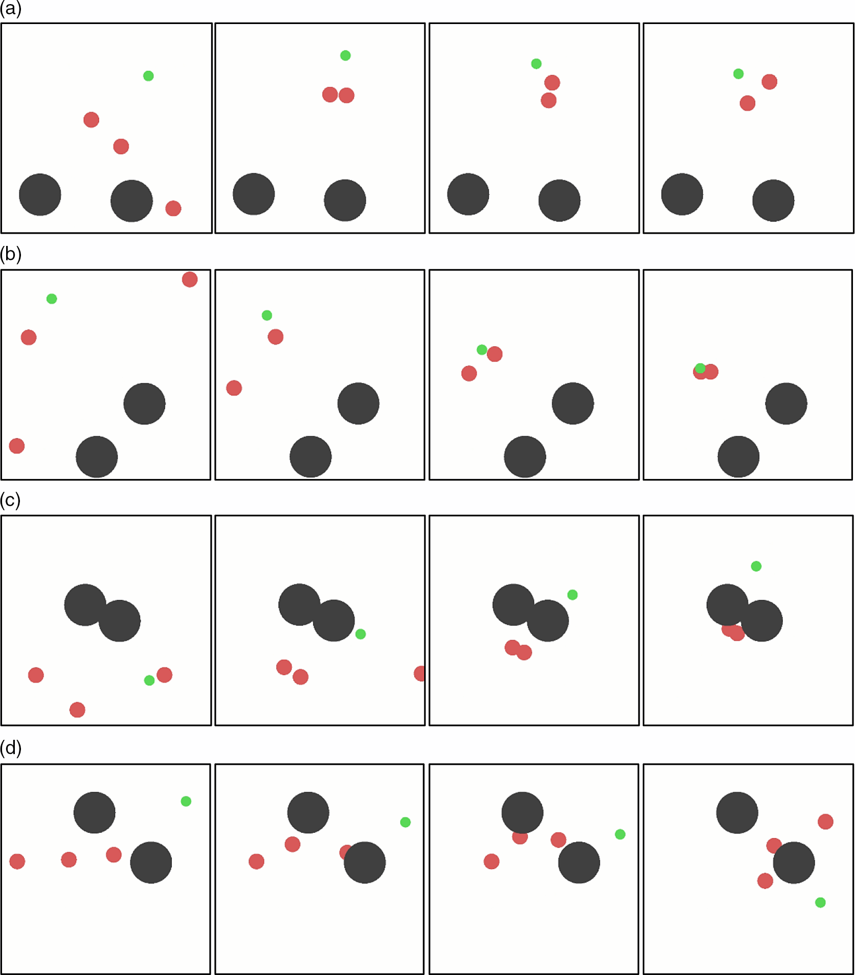
Figure 12. The training process for round-up and confrontation with the original MADDPG algorithm. (a) and (b) are two randomly generated scenarios, in which one agent is lost, which fails to better reflect the collaborative characteristics of the cluster. (c) and (d) are two randomly generated scenarios, in which the agents frequently collides with obstacles, so the operation safety cannot be well guaranteed.
6.0 Conclusions and Future Work
This paper proposed a new improved Multi-Agent Reinforcement Learning algorithm, which mainly improved the learning framework and reward mechanism based on the principle of MADDPG algorithm. The action variables are introduced into Q network and P network, and used for calculation of Q value together with the state variables. The structure of Q network and P network in the new framework are no longer the same. The number of network nodes can be adjusted according to the training results. In addition, the reward mechanism is also improved. The obstacle avoidance settings are added to effectively improve the survival rate of UAV cluster. At the same time, the control of each UAV in the cluster is added, which greatly improves the ability of cooperative combat. Integrating the above improvements, the improved MADDPG algorithm is able to calculate Q values more precisely, which can also benefit the learning of optimal policy. In order to verify the feasibility of the improved MADDPG algorithm, we constantly adjust through a large number of simulation tests, and finally achieved good training results.
One disadvantage of the algorithm is that its real-time performance can not meet the actual combat requirements. And with the increase of the number of clusters, the amount of computing information increases exponentially, which makes the real-time performance of the calculation worse. We preliminarily assume that Deep Learning and Reinforcement Learning can be combined to solve the real-time problem. Through a large number of simulation experiments to accumulate data, and introduce deep learning module to learn these prior knowledge. Then use reinforcement learning to conduct online decision-making training, which is helpful to improve their independent decision-making ability. Another weakness is that the algorithm can only apply to the problem of a fixed number of agents. In actual combat, it is very likely that the loss of the UAVs in the cluster will always occur, so the development of a variable number of agents algorithm will be the next problem to be solved. We leave these two problems to future work.
Acknowledgement
This work was partially supported by the National Natural Science Foundation of China (Nos. 11872293, 11672225), and the Program of Introducing Talents and Innovation of Disciplines (No. B18040).
Supplementary material
To view supplementary material for this article, please visit https://doi.org/10.1017/aer.2021.112


