NOMENCLATURE

λ _B

Bragg weavelength

n_eff

effective refractive index

Λ

grating period

Δλ _B

Bragg wavelength shift

p₁₁ & p₁₂

Pockel’s coefficient

v

Poisson’s ratio

Δε

strain

T

training set

a_i

training attributes

t, b_i,b_ij

training targets

c_j, τ _j

decoding variable

2.0 SHAPE ESTIMATION METHODOLOGY

2.1 Sensing principle

Fiber Bragg Gratings are photo-induced Bragg reflectors which are equal to created by a periodic refractive index change induced by the interference pattern of an intense UV light within the core of the optical fiber. When a light of broadband spectrum is launched into an FBG structure, a singular wavelength is reflected back and the rest is transmitted through. The wavelength reflected is governed by the relation:

(1) $${\mib{\rlambda }} _{{\mib{B}} } {\equals}2{\mib{n}} _{{{{\bf eff}} }} {\mib{\Lambda }}$$

where n _eff is the effective refractive index of the core and Λ denotes the Bragg grating pitch or the distance between each successive refractive index change. Under the influence of strain, the value of Λ increases or decreases depending upon the nature of strain. The dependence of the change in the reflected wavelength with respect to the change in strain is given as⁽ Reference Erdogan ^{20 )}

(2) $$\Delta {{\rlambda }} _{{\mib{B}} } {\equals}{{\rlambda }} _{{\mib{B}} } \left( {1{\minus}\left( {{{{\mib{n}} _{{{\bf{eff}} }}^{2} } \over 2}} \right)\left[ {{\bf p}_{{12}} {\minus}{\rm \rnu }\left( {{\bf p}_{{11}} {\plus}{\bf p}_{{12}} } \right)} \right]} \right){\mib{\Delta {\repsilon}}}$$

where λ _B is the central reflection wavelength of the FBG under no strain conditions, p ₁₁ and p ₁₂ are Pockel's coefficients, Δε is the amount of strain impressed upon the structure and ν is Poissons' ratio of the material. One of the distinctive advantages of FBGs is that it requires only a single-ended connection to a control system. In this article, to address the issue of fault tolerance in a serially multiplexed sensor array setup, the connection has been made via both ends. This is to ensure that in the event of an optical link breakage, the light can still be launched into the series of sensors beyond the break point. FBGs can also be multiplexed in large numbers to cover for a greater area of the structure.

2.2 Multi target single model SVR

SVMs are a class of pattern recognition techniques that can be used for both classification and regression. SVMs operate by incorporating a ‘kernel trick’. This trick transforms the data to a higher dimension that allows linear separability. The data set for training can be represented by⁽ Reference Chang, Hsieh, Chang, Ringgaard and Lin ^{21 )}

(3) $${\bf{T}} {\bf {\equals}\bigg\{ \left( {a_{i} ,t} \right)\left| {a_{i} {\bf \in}\Re ^{h} ,t{\bf \in}\Re \bigg \} _{{({\bf i}{\equals}1)}}^{{\bf n}} }} \right.$$

where a _i is the input vector attribute and t is the training target. a _i is defined as the training input vector containing ‘h’ elements, and ‘n’ is the total number of training instances. Statistically, it can also be shown that any non-linearly separable data in lower dimensions can become linearly separable in a sufficiently higher dimension. In the present work, to estimate the deflection profile of the simply supported beam and the aircraft wing structure, it is necessary to predict the displacement values along a greater number of locations. Hence, the training data for such a training set can be written as

(4) $${\bf T}{\equals}\left\{ {\left( {{\mib{a}} _{{\mib{i}} } ,{\mib{b}} _{{\mib{i}} } } \right){\rm \,\mid\,}{\mib{a}} _{{\mib{i}} } \in\Re ^{{\bf h}} ,{\mib{b}} _{{\mib{i}} } \in{\mib{c}} _{{\mib{j}} } \forall \left[ {{\mib{c}} _{{\mib{j}} } \in\Re } \right]_{{{\bf j}{\equals}1}}^{{\bf m}} \,\mid\,{\bf m}\,\gt\,{\rm h}} \right\}_{{{\bf i}{\equals}1}}^{{\bf n}}$$

where a _i and b _i are the training vectors and the corresponding training targets, respectively. Each training target contains ‘m’ attributes, which are individually denoted by c _j , that correspond to the number of locations on the beam where the deflections are monitored. Conventional SVR requires training to be performed according to the data set represented by (3). The proposed technique uses the appropriately trained SVR model to estimate 30 different values corresponding to the input condition in the experimental setup for evaluating the bending of a simply supported beam. The same has also been performed for a model aircraft wing, by monitoring and estimating for 180 locations along both surfaces of the wing. Simulations have been performed for the simply supported beam only, and the results for Technique C is hereby shown in comparison with the same for the experimental data. For the purpose of simulations, the deflections and the amount of strain at different lengths of a simply supported beam have been calculated from the beam bending equations. Only Technique C has been simulated for reasons mentioned later. The amount of strain at three distinct locations on the beam (simulated positions of the FBGs) have been used to modify the Bragg conditions and find the wavelength shift as per Equation (2). The wavelength shift in combination with the appropriate DV of Equation (6) has been used to generate the training attributes of the training vector of the ANN. The target vector was composed of the 30 displacement values obtained from the beam bending equations above. The strain and deflections of the beam has also been simulated for loading at different positions, and the appropriate training and target vectors were generated for each condition to formulate the training set mentioned in Equation (5). In this endeavour to investigate the capability of the SVR model to operate under real-life conditions, the training set was not subdivided into training, validation and cross validation, like conventional approaches. Instead, the entire training set was used for the purpose of training the proposed SVR model and testing conditions were generated in the afore-mentioned manner, by simulating the placement of weight on the simply supported beam at the central and one random position. The simulation has not been performed for Technique A, as the methodology already uses the beam bending equations to estimate the loading point and hence would provide trivial results. Technique B is also incompatible with the simulation as the multiple number of models pertaining to positions on the simulated beam, would also provide trivial solutions for each location. The experimental procedure, shown in Fig. 3, was conducted in the same manner as the simulation. The data recorded from the OSA (for the wavelength shifts of the FBG) and the appropriate DVs were used to generate the attributes of the training vector. The corresponding displacements recorded from the travelling microscope at 30 locations have been used to formulate the attributes of the target vector, respectively. In Equation (4), the training vector also corresponds to the representative training data set for multi-output ANNs. In order to train the SVR model for the purpose of displacement profile estimation/shape sensing, two techniques (A and B) for training can be used and their corresponding flowcharts are shown in Fig. 1(a) and (b), respectively.

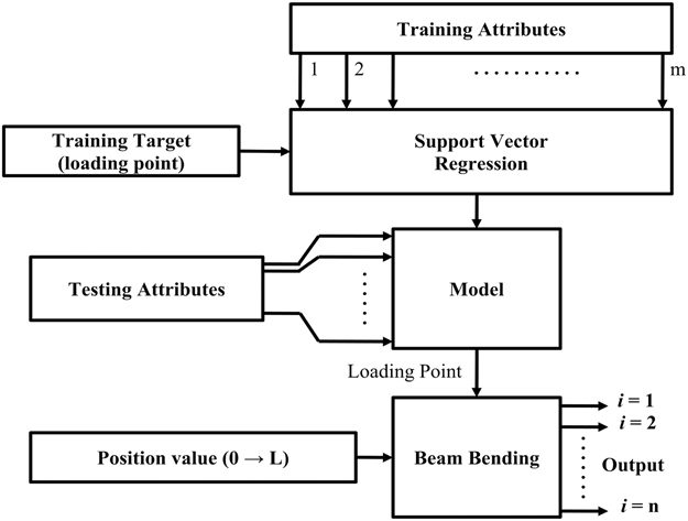
Figure 1 (a) Shape estimation using SVR and beam bending equations (Technique A).

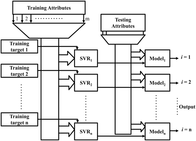
Figure 1 (b) Shape estimation using multiple parallel SVR models (Technique B).

Technique A estimates the loading point depending on the FBG wavelength shifts. The loading point is then used to deduce the shape profile of the beam. The beam bending equations require the location on the beam where the displacement and the strain is to be evaluated. The same is provided by a sequential input of values, denoted by the position values (0 to L) in Fig. 1(a). Technique B determines the displacement of each of the 30 locations along the length of the beam simultaneously, using a separate SVR model for each location. Technique B allows each SVR model to learn the non-linearities associated with each location. Both the techniques favor conventional training, where the SVR uses one exclusive target value for a set of input wavelength shifts using the representative training data set given by (3).

Alternatively, we have modified the required training set, given by (4) as the following:

(5) $${\bf T}{\equals}\left\{ {\left( {\left[ {{\mib{a}} _{{\mib{i}} } ,{{\rm \rtau }} _{{\mib{j}} } } \right],{\mib{b}} _{{{\mib{ij}} }} } \right){\rm \,\mid\,}\left[ {{\mib{a}} _{{\mib{i}} } ,{\mib{\rtau }} _{{\mib{j}} } } \right]\in\Re ^{{{\bf h}{\plus}1}} ,\left[ {{\mib{b}} _{{{\mib{ij}} }} \in\Re } \right]_{{{\bf j}{\equals}1}}^{{\bf m}} } \right\}_{{{\bf i}{\equals}1}}^{{\bf n}}$$

where τ _i is the additional variable denoted as the ‘Decoding Variable’ (D.V.). The D.V. value cycles over the number of attributes present in the target set corresponding to a given training vector. For the present work, two separate D.V. structures have been chosen for the simply supported beam setup (6) and for the aircraft wing structure (7) as follows:

(6) $${\mib{\rtau }} _{{\mib{j}} } \in\left[ {1,30} \right];\left\{ {{\mib{\rtau }} _{{\mib{j}} } {\equals}{\rm Deflection \ at \ location }'{\bf j}'} \right.$$

(7) $${\mib{\rtau }} _{{\mib{j}} } \in\left[ {{\bf a},{\bf b}} \right]\left\{ {\matrix{ {a\in\left[ {1,2} \right], \left( {1{\minus}{\rm Upper}\,{\rm Surface; 2{\minus} Lower}\,{\rm Surface}} \right)} \cr \!\!{b\in\left[ {1,90} \right],\left( {9{\rm 0 }\,{\rm spatial}\,{\rm locations}\,{\rm along}\,{\rm a}\,{\rm surface}} \right)} \cr } } \right.$$

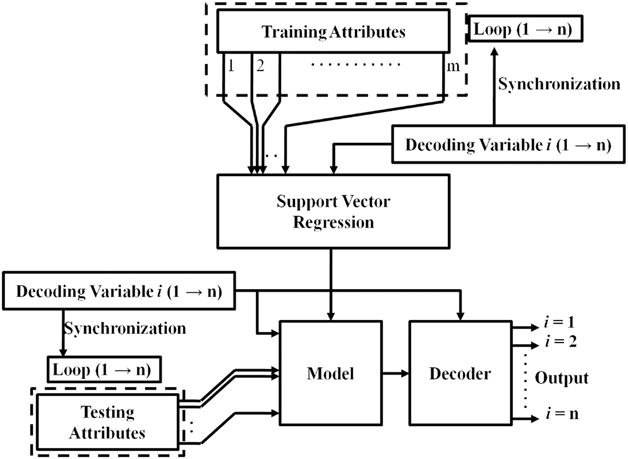
The flowchart for the training and the testing using our proposed bio-inspired Technique C is shown in Fig. 1(c).

Figure 1 (c) The novel SVR training method for shape profile estimation (Technique C).

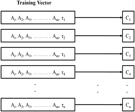
The method reduces the more complex training set given by (4) into a sequence of simpler training sets as depicted in Fig. 2(a) and (b). The proposed technique of modifying the training dataset is drawn from the observed way in which the human brain operates. There has been a considerable amount of study both from a medical perspective, which shows how the different parts of the brain activates and deactivates in response to different thought processes and stimuli. This specific field of study has accelerated considerably with the development of functional Magnetic Resonance Imaging (fMRI) of the brain⁽ Reference Jahn, Deutschländer, Stephan, Strupp, Wiesmann and Brandt ^{22 ,} Reference Marx, Deutschländer, Stephan, Dieterich, Wiesmann and Brandt ^{23 )}. The location and the intensity of the brain activation and deactivation patterns are determined by the type and the magnitude of the stimulus. Due to the incredibly complex interconnected nature of the different parts of the brain, it is currently of limited knowledge as to which locations are influenced by what stimuli in which manner, but different classes of stimuli produces different effects and hence affects different parts of the brain. The proposed technique is very similar to how different parts of the human brain activates in response to the varying stimulus and environmental conditions. The D.V. introduced in Technique C provides a unique ‘stimulus’ to the SVR, aside from the other attributes of the training vector. The D.V. (τ _i ) allows the model to switch to the different outputs necessary, for a given set of wavelength shifts. This becomes similar to requiring an output for different stimuli, although the interpretation from an engineering perspective can be used in a repetitive sequence, to generate the displacement map of an entire structure. This procedure saves time and computational resources (due to the use of a single model instead of multiples), without sacrificing the required accuracy. The analogue between the operation of the human brain and the presently proposed ‘bio-inspired training technique’, is significantly more apparent in the use of ANN, than with SVR, but a more thorough investigation is beyond the scope of the present article. Comparative results with SVR and ANN for the same task have been provided later.

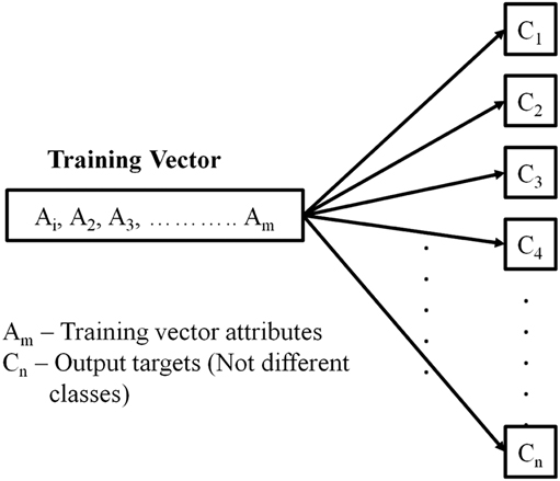
Figure 2 (a) The one to many mapping problem for shape profile estimation.

Figure 2 (b) Reduction of the one-to-many problem to a one-to-one mapping problem using the D.V. τ _j

In our work, shape sensing on a simply supported beam has been performed as a proof-of-concept, and the same on an aircraft wing sample as a probable application using the bio-inspired SVR method. Thirty locations along the beam and 180 locations along both the surfaces of the aircraft wing sample had been identified, whose displacements were considered as the target elements for training of the SVR model. For the simply supported beam, three FBGs were attached at different locations and interrogated using the OSA. For the aircraft wing sample, five FBGs were used in conjunction with an FBG interrogator working to develop the wing shape profile. The wavelength shifts of the FBG sensors have been considered as the attributes of the input vector. Depending on the position of loading, the beam would have a certain deflection profile whereas the amount of deflection at the free end of the wing sample depends on the amount of weight placed on it. The combined data containing the wavelength shifts of the FBGs and the DVs were used as the training data and the deflections at the respective locations were used as training targets for the SVR model.

3.0 EXPERIMENTAL SETUP

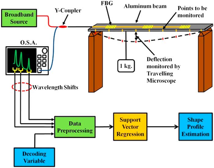
The experimental setup shown in Fig. 3 consists of a simply supported aluminum beam (750 mm×20mm×3 mm), with three FBGs mounted on it. The three FBGs (1538.32nm, 1544.89nm and 1551.2nm) were serially multiplexed on the beam at 187, 375 and 562 mm approximately from the left end of the aluminium beam. The FBGs were fabricated using phase-mask technique by Central Glass and Ceramic Research Institute (C.G.C.R.I.), Kolkata.

Figure 3 Experimental setup to generate the training and testing data for shape profile estimation of a simply supported beam.

A broadband source (Denselight DL-BX9-CS5254A) having a central wavelength of 1540nm a full width at half maximum (FWHM) of 35–40nm was used to launch the light into the FBG array via a Newport Y-coupler. The reflected signal from the FBGs was displayed using an Optical Spectrum Analyzer (Yokogawa AQ6317C). A 1 kg weight was hung at different distances from one of the supports, in the simply supported beam experiment. This causes the center of the beam to deflect by different amounts and also creates a distinctive deflection profile for each instance. Simultaneously, the deflections of the 30 locations along the length of the beam were monitored using a travelling microscope. The training data composed of 25 training vectors and the corresponding training targets. Each training vector comprises of the three wavelength shifts of the FBGs as recorded from the OSA and the D.V.s. The training targets comprise thirty deflections monitored along the length of the beam, corresponding to a single loading position. Testing data were gathered for several instances (which includes central and non-central loading). The deflection values along the beam were also recorded for these two instances to check for the proficiency of the proposed SVR model. A SVR Library (LibSVM v3.16)⁽ Reference Chang and Lin ^{24 )} was used to develop the SVR model and implement the shape sensing algorithm. The testing conditions have been chosen for loading at 37.5 cm and 20 cm from the left support to compare the efficiency and computational requirement of the different techniques. The wavelength shifts and deflection profile for 25 different locations of loading were used for training the different models of the different techniques.

In the second example, an aircraft wing model has been setup in a cantilever configuration. The aircraft wing shape estimation has been developed to show the applicability of the SVR for practical applications using the bio-inspired training method. It also shows the dimensional scalability of the proposed Technique C to accommodate three dimensional complex surfaces which may benefit automated shape estimation systems. A total of 3,000 points along both surfaces of the wing were monitored for recreating the shape of the wing in the computer, for each loading instance. Of these, 180 locations (90 along each surface) were used for training and testing of the SVR model. To monitor such a large number of locations, at an instance, photogrammetry was used. Two types of deflection mechanisms – namely bending and twisting have been performed, by applying the necessary force at the free end. The images of the perturbed state of the wing were captured using a Canon S2IS 5MP digital camera. The experimental setup shown in Fig. 4(a) includes the cantilever setup as the aircraft wing model.

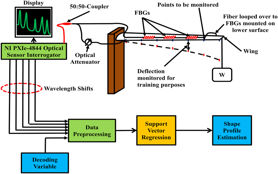
Figure 4 (a) Experimental setup to generate the training and testing data for shape profile estimation in an aircraft wing model.

The wing planform with a 35° leading edge sweep was mounted with five different FBGs (1,526nm, 1,536nm, 1,546nm, 1,556nm and 1,566nm) as shown in Fig. 4(b). W denotes the weight placed at the edge of the cantilever setup used to bend the wing. The FBG array was a Micron Optics 5-sensor FBG array (os1200) with a sensitivity of approximately 1 pm/µstrain. The FBG interrogator was a National Instruments PXIe-4844 Optical Sensor Interrogator operating at a maximum frequency of 10 Hz with four channels over a wavelength range of 1,510–1,590nm. Eight training vectors and three testing vectors consisting of the individual wavelength shifts of the five FBG sensors and the necessary DVs as given by (7) were generated from the experimental setup. Each target vector contains the deflection values (90 locations on either surface), which were used to develop the displacement field and hence the shape of the wing. The training and testing of the SVR models for the different simulations and the experimental setup have been carried out on an ASUS K53SV-SX521D Laptop (Intel Core i7-2670QM having 4 cores, 8 threads, 8 GB RAM and 750 GB HDD).

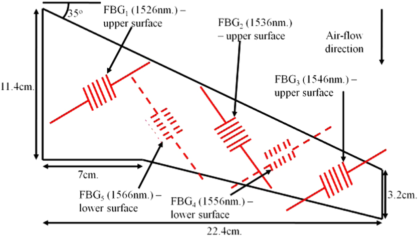
Figure 4 (b) The wing planform and the position of the five FBG sensors.

4.0 RESULTS AND DISCUSSIONS

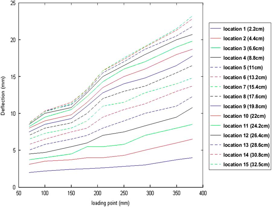
In the present work, the deflection profile of a simply supported aluminum beam for loading at 37.5 cm and 20 cm has been evaluated from the left support using the three techniques as mentioned earlier. The aluminium beam was loaded at different positions along its length to obtain different deflection profiles. The wavelength shifts recorded from the OSA, along with the D.V.s were used to develop the necessary training data for the SVR model. Figure 5 shows the non-linearities in 15 of the 30 monitoring locations along the beam for different instances of loading.

Figure 5 Non-linearities exhibited by 15 of the 30 monitored locations along the beam for varying positions of loading.

The significant non-linearities exhibited at different locations of the beam due to loading at different locations are due to the inhomogeneity of the beam (i.e. change in the physical dimensions of the beam – length, breadth and thickness). Such a sample is also used to show the inadequacy of Technique A and promote the advantages of Technique C (i.e. to learn the unique non-linearities from the recorded data and provide a more accurate result).

Figure 6 shows the reconstruction of the shape of the beam for the two loading conditions, using the training as mentioned in Techniques A and B.

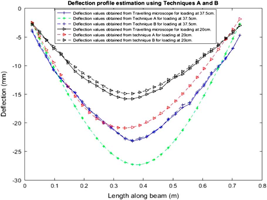
Figure 6 Shape estimation of the simply supported beam using Techniques A and B.

It may be seen that Techniques A and B, although favoring the conventional SVR training techniques, may not provide accurate results or be computationally efficient, as discussed later. Figure 7 shows the reconstructed deflection profile from experimental analysis using our proposed Technique C.

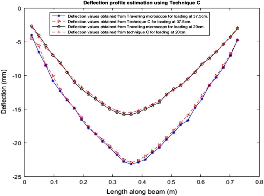
Figure 7 Shape estimation of the simply supported beam using Technique C.

The physical displacements recorded using a travelling microscope, shows deviation from a smooth bent beam at some locations along the length of the beam. This is directly related to the displacement non-linearities at different location, which has been experimentally verified as shown in Fig. 5. Due to the positional non-linearities, there exists displacement jumps from one position of the beam to the next, giving the impression of non-smoothness as depicted in Figs 6 and 7. Technique C can be seen to provide a viable alternative to both Technique A (which lacks in accuracy) and Technique B (which is computationally more resource intensive), as summarized in Table 1.

Table 1 Shape estimation of simply supported beam using Techniques A, B and C

^a The MSE for Techniques A and B have very low values as the SVR model trains to predict only one value but for Technique C, there are model trains for 30 outputs per input vector.

^b There are no regression values for Techniques A and B as the number of outputs per model is only one, but in Technique C, there are 30 values per model per instance.

For comparison with Techniques A and B, only the experimental results of Technique C have been shown in Fig. 7. Despite having a lower MSE, Technique A provides the lowest model file size and prediction time, but also suffers the greatest error. This is attributed to the fact that Technique A fails to take into account the non-linearities of an experimental setup. Technique B, provides the lowest MSE, but has a higher prediction time and model file size, and hence the best result. Consequently, it also requires greater computational resources. The latter is because of the fact that the multiple SVR models need to be executed simultaneously to yield the shape of the beam. Technique C has been shown to successfully reconstruct the shape of the beam for both simulation and experimental instances. The MSE of the experimental procedure of Technique C can be directly compared with the simulated MSE of Technique C. The difference between the above-mentioned quantities, may be attributed to the fact that random non-linear displacement conditions were not considered for the simulation, making the results of the simulation considerably more accurate. However, the experimental MSE of our proposed method is at par with that of Technique B. The training time required for Technique C is at par with Technique B due to the large number of exclusive training instances generated by the introduction of the DVs***. Thus, from Table 1, it may be ascertained that Technique C preserves the advantages of both Techniques A & B. because of its unique bio-inspired training scheme, the proposed technique C requires significantly lower computational resources (processing power and storage space) yet maintains a similar if not greater value of accuracy and a lower prediction time. It must also be noted that the present experiments were scaled down for execution in controlled environments. Hence in terms of quantifiable errors, the values presented in this article are of the order of 10^-2%. These values would increase as the experimental setup sizes are increased and/or due to the greater amount of non-linearities present. However, it may be observed that the errors provided as part of the experimental verification is an order of magnitude higher than that provided by the simulation, as shown in Table 1. Another significant reason for such low error values, is the choice of the Pattern Recognition Algorithm that has been implemented. SVR is a highly complex statistical technique that operates on a higher numerical dimension, and hence can accommodate experimental non-linearities. This is also one of the causes of low error values in the results documented in Table 1 and 2. The use of an ANN to perform the same task, has been provided as a comparative benchmark. However, it must be noted that an ANN is significantly more malleable in its operation than an SVR model. The accuracy of the ANN would depend upon the number of hidden layers, no. of neurons in each hidden layer, no. of simultaneous outputs and even the activation function of the individual layers. For the present scenario, a two hidden layer network, employing 10 neurons each, having a tan-sigmoid activation function, with a singular output neuron having a linear activation function has been used.

Table 2 Wing Sample Shape Estimation using Technique C

The inherent advantages portrayed by Technique C, with respect to conventional methods, indicates that it is well suited for several real-life applications. For this article we propose its use as an integral part of a non-visual, non-tactile shape estimation mechanism in aircraft wings.

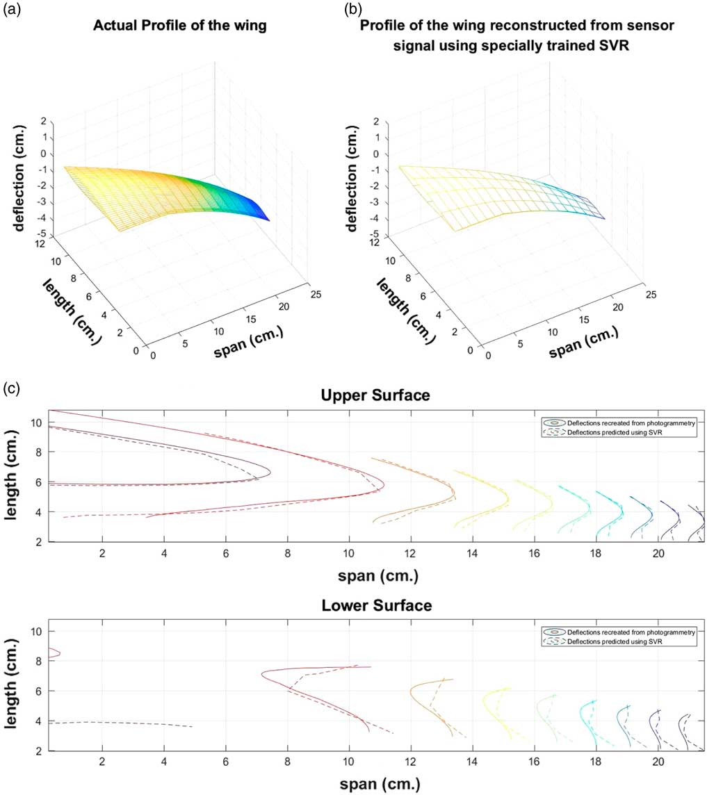
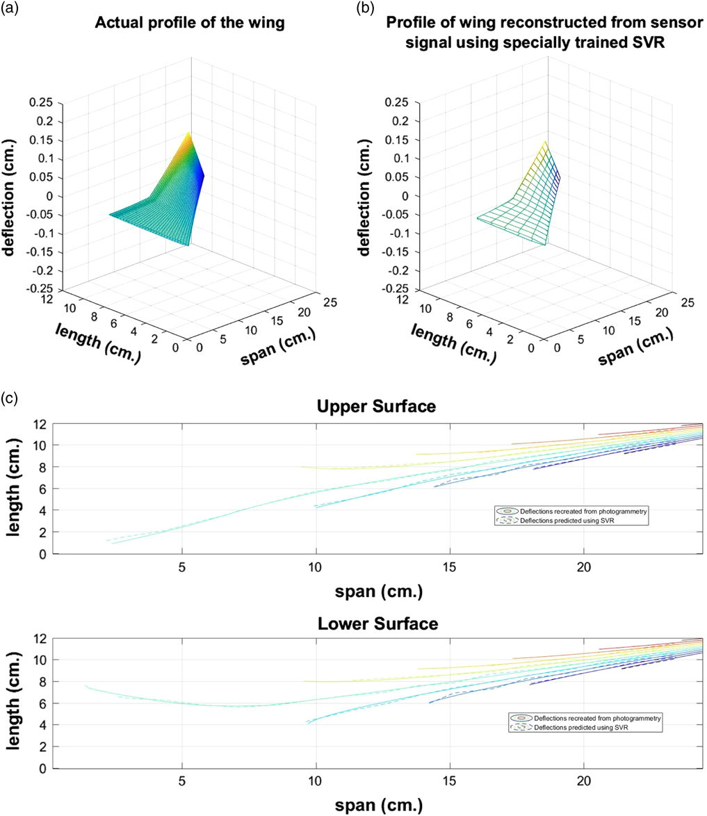
From Figs 8, 9 and 10, it may be seen that the proposed single model training technique (Technique C), can be effectively utilized for two-dimensional shape sensing of complex surfaces. Table 2 provides the summary of the computational performance of the single SVR model for the three wing samples shape sensing instances shown in the above-mentioned figures. Table 2 also shows that the proposed training method can preserve its accuracy and computational efficiency, despite an increase in the dimensionality of the shape estimation problem.

Figure 8 The shape of the wing (a) Deduced from photogrammetry and (b) reconstructured by the proposed SVR model and (c) the overlaid contour maps of the upper and lower surfaces of the wing as determined from photogrammetry and reconstructed by the proposed SVR model.

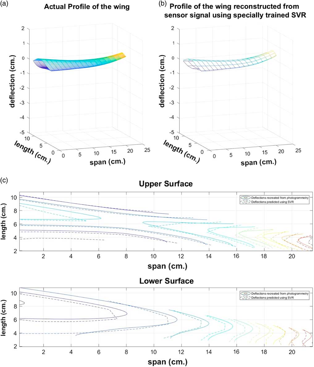
Figure 9 The shape of the wing (a) Deduced from photogrammetry and (b) reconstructured by the proposed SVR model and (c) the overlaid contour maps of the upper and lower surfaces of the wing as determined from photogrammetry and reconstructed by the proposed SVR model.

Figure 10 The shape of the wing (a) Deduced from photogrammetry and (b) reconstructured by the proposed SVR model and (c) the overlaid contour maps of the upper and lower surfaces of the wing as determined from photogrammetry and reconstructed by the proposed SVR model.

It may be noted that the training time for all the prediction instances remains the same. This is because the appropriate model was trained only once, with all the instances of bending and twisting. Hence the time period for training, size of the model file, No. of training vectors, no. of training attributes and the no. of outputs remain same. However, the prediction time can be seen to vary for the three different instances, due to available computational resources and the instantaneous speed of the computational system.

To aid in the fault tolerance of serially multiplexed sensors, it was decided to use both ends of the fiber to launch the light as shown in Fig. 4(a). Since the sensor array is placed in a loop, both the reflective and the transmitted spectrum of the FBG would be impressed upon the interrogation mechanism, thereby reducing the FBG signal strength and hence the effectiveness of the system. For this reason, an optical attenuator is incorporated along one fiber direction entering into the FBG array. Under normal operational circumstances, the attenuator would be active, thereby blocking the launch of the light from one end. But in the event of an optical link breakage, the attenuator can immediately be turned off, allowing the light to reach the sensors which were beyond the location of the optical link disruption and hence could not be interrogated under normal circumstances.

The proposed single model multi-output training method for SVR has shown a comparable accuracy with present techniques albeit with reduced computational resources. Further an increase in the dimensionality of the problem (i.e. from 2D surfaces to 3D solids) may be implemented by a change in the structure of the D.V. array. This would allow the system to be scaled to accommodate additional hardware (i.e. sensors), or retrain the system to provide enhanced features for a given set of hardware elements. The methodology would improve both economics and logistics of operation. It may also be used as part of a soft-sensor approach for high accuracy, multiple objective embedded sensing instrumentation. For the present work, SVR has been chosen over ANNs, as the number of training instances were small. However, such a form of training may also be used for ANNs employing a different network architecture for different purposes which includes shape sensing. The proposed technique may be extended for other Quasi-Distributed sensing systems having a lower number of sensors but requiring a greater area of coverage and higher resolution. The presently proposed training technique is also a candidate for the development of ‘Fly-by-Feel’ (FBF) capability for aircrafts. It would enable aircrafts to have an independent sensing system, which can also be coupled with standard Fly-by-Wire control systems to inform the avionics system as well as the pilots to the physical state of the aircraft in real-time. An FBF system, can be an adaption of the present generation of integrated sensing system used on the current generation of aircrafts, but modified to provide direct structural information for physics based adaptive flight control.