NOMENCLATURE
- h
flight height
- R
distance between the formation system and the target
- L
distance between sub-vehicles
- F
distances between the 1th flight vehicle m 1 and the other three ones
 $\boldsymbol{x}_{\boldsymbol{s,i}}$
position vector
- $\textbf{\textit{v}}_{\boldsymbol{s,i}}$
velocity vector
- $\textbf{\textit{a}}_{\boldsymbol{s,i}}$
acceleration command vector
- $\textbf{\textit{d}}_{\boldsymbol{s}}$
external disturbance
- $\textbf{\textit{x}}_{\boldsymbol{q,i}}$
expected position vector in the LOS coordinate system
- $\textbf{\textit{v}}_{\boldsymbol{q,i}}$
expected velocity vector in the LOS coordinate system
- $L_{23}, L_{24}, L_{34}$
baseline length between each sub-vehicle
- $L_{0}$
distance between the 1th sub-vehicle and the plane T 2T 3T 4
- $\Delta center$
offset angle
- $\textbf{\textit{e}}_{\textbf{1},i},\textbf{\textit{e}}_{\textbf{2},i}$
position error vector and velocity error vector
- $\textbf{\textit{s}},\textbf{\textit{s}}_{1},\textbf{\textit{s}}_{2}$
sliding mode surfaces
- $\beta, \gamma$
sliding mode parameters
- $k_{1}, k_{2}, \rho, \eta$
control law gains
- $\textbf{\textit{a}}_{\textbf{\textit{s}}}$
non-singular terminal sliding mode control law
- $\delta, \delta\hat{}$
upper limit and estimate of disturbance
- $\varepsilon_{1}$
small normal number
- $\textbf{\textit{V}},\textbf{\textit{V}}_{1},\textbf{\textit{V}}_{2}$
lyapunov functions
- $T_{reach}$
reach time
- $\tau$
delay time constant of autopilot
- $\textbf{\textit{a}}_{\textbf{\textit{m,i}}}$
the acceleration vector in the LOS coordinate system
- $k_{0}$
control parameter
- $t_{r}$
desired time
- $\textbf{\textit{z}}_{\textbf{\textit{0}}}, \textbf{\textit{z}}_{\textbf{\textit{1}}}, \textbf{\textit{z}}_{\textbf{\textit{2}}}$
estimations of disturbance observer
- $\lambda_{0}, \lambda_{1}, \lambda_{2}$
observer gains


1.0 INTRODUCTION
The complex battlefield environment and the development of integrated anti-missile defense technology make the attack mode of single flight vehicle severely challenged; thus the cluster cooperative operation system is being introduced into future war(Reference Wang, Zhang and Wu1–Reference Wang and Lu3). The collaborative operation of multiple flight vehicles means that all members are formed into a combat network to conduct the real-time information interaction through a data link, so as to improve the anti-interference ability of the formation system and enlarge the cooperative detection probability to the target during the mid-guidance stage(Reference Wang and Lu3). After entering the terminal guidance stage, the collaborative system can realise the saturation attack on the target(Reference Li, Lin and Wang4). For advanced reentry vehicles equipped with radar detector, which have high flight speed and wide flight airspace. For this kind of flight vehicle, such as anti-ship missile with radar seeker, they gain the target information using own sensor or leader’s sensor in the cooperative case and then fly to the target relying on guidance command. In order to ensure the high-precision co-positioning of the target after the detectors are turned on, it is necessary for all flight vehicles to pull apart the required space distance and angle during the mid-guidance stage and then adjust the attitude of the projectile body to align the target.
As an important part in the process of cooperative combat, the formation flight control of multiple flight vehicles has attracted the attention of scholars. The formation technology of multiple flight vehicles was firstly applied to the under-actuated mechanical system such as spacecraft and UAV, and lots of research outputs were produced. A decentralised scheme for spacecraft formation flying via the virtual structure approach is proposed in Refs (Reference Sabol, Burns and Mclaughlin5) and (Reference Ren and Beard6). As the extension of this study, the authors in Ref. (Reference Nazari, Butcher, Yucelen and Sanyal Yucelen7) studied the decentralised consensus control of a formation of rigid body spacecraft in the framework of geometric mechanics while accounting for a constant communication time delay between spacecraft. In the field of UAV, the main formation control technologies include model predictive control, bionic algorithm and consistency theory, and the consistency control algorithm based on graph theory gradually becomes the focus of research. Numerical research results are available for Refs (Reference Ghommam and Luque-Vega8–Reference Huang and Sun12).
Due to the difference in physical structure and motion mechanism, there are huge differences between missiles and UAVs in formation flight control, and the corresponding research results are still lacking. The formation tracking protocols were proposed by using the ideas of proportion and differential controller for the multiple BTT missiles system(Reference Cui, Wei, Guo and Zhao13) and multiple aircrafts system(Reference Rezaee and Abdollahi14). Wei et al.(Reference Wei, Guo, Lu, Shi and Zhang15) designed an adaptive controller to compensate the coupling effects caused by attitude motion. The dynamic surface controllers were introduced for solving the formation tracking issues for multiple missiles system in Ref. (Reference Wang, Liu and Tian16). In Ref. (Reference Wei, Shen, Ma, Guo and Cui17), cost functions were defined by considering the formation tracking error and control input, and the optimal formation tracking protocol can be obtained by using the functional calculus of variation, where the velocity and flight path angle were defined as the input vector.
Based on the high-precision positioning requirement of multiple flight vehicles for the target in a long distance, this paper mainly focuses on the cooperative control law design of formation configuration. The structure of this paper is organised as follows. In Section 2, the problem statement is provided, and the kinematics models of the flight vehicles are also built. Next the configuration parameters that satisfy the constraints are designed in the Section 3. The control law with considering the effects of the external disturbance and the first-order dynamic characteristic of the autopilot is designed, and a novel improved control method is proposed in the Section 4. Simulation results and analysis are shown in the Section 5. Finally, the concluding remarks are offered in the last section.
2.0 PROBLEM FORMULATION AND MATHEMATICAL MODEL
Considering the following scenario that multiple flight vehicles are scatted by a parent vehicle at a certain height
 $h$
, and all flight vehicles can be numbered as
$h$
, and all flight vehicles can be numbered as
 $i=1,2,...,n$
to easily subsequent descriptions. Obviously, these sub-vehicles would perform inertial flight in the absence of control, so the system configuration cannot be guaranteed to achieve high-precision cooperative detection during the mid-guidance phase. Therefore, it is assumed that if the finite time convergent control strategy is designed to make all sub-vehicles form the expected distances and angles at the preset distance
$i=1,2,...,n$
to easily subsequent descriptions. Obviously, these sub-vehicles would perform inertial flight in the absence of control, so the system configuration cannot be guaranteed to achieve high-precision cooperative detection during the mid-guidance phase. Therefore, it is assumed that if the finite time convergent control strategy is designed to make all sub-vehicles form the expected distances and angles at the preset distance
 $R$
between the formation system and the target, and then maintain the configuration before the terminal guidance phase. Combine with the characteristics of detection device, the space formation constraints are listed as follows(Reference Zhao, Chao and Wang18,Reference Ratnoo and Shima19) :
$R$
between the formation system and the target, and then maintain the configuration before the terminal guidance phase. Combine with the characteristics of detection device, the space formation constraints are listed as follows(Reference Zhao, Chao and Wang18,Reference Ratnoo and Shima19) :
-
(1) Configuration constraints. Assume that
$n=4$
, and then these four sub-vehicles can be named as
${m_1},{m_2},{m_3},{m_4}$
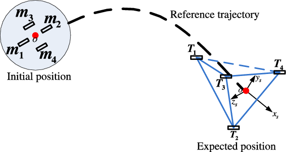
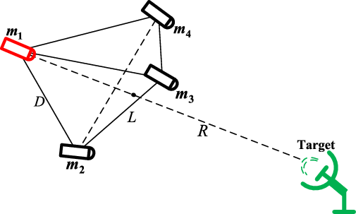
. These four sub-vehicles form the tetrahedron structure, as shown in Fig. 1, where the
${1^{th}}$
flight vehicle in the back and the other three in the front; The connection line between the
${1^{th}}$
one and the target is basically perpendicular to the plane where the other three ones are located in, and the offset angle relative to the centre of the plane cannot over
$10\% $
.Figure 1. Relative position between system configuration and target.
-
(2) Distance constraints between sub-vehicles (
${m_2},{m_3},{m_4}$
). Considering the operating distance of the radar detection device, choose
$R=300{\mathop{\rm km}\nolimits} $
. Besides, to guarantee the positioning accuracy indexes of configuration system, choose
$L \ge 6{\mathop{\rm km}\nolimits} $
; the distances between the
${1^{th}}$
flight vehicle
${m_1}$
and the other three are not more than
$10{\mathop{\rm km}\nolimits} $
, i.e.
$D \le 10{\mathop{\rm km}\nolimits} $
; the distance between the
${1^{th}}$
flight vehicle and the plane formed by the other three sub-vehicles satisfies
$1.5\sim 3.5{\mathop{\rm km}\nolimits} $
.


For the formation control of multiple flight vehicles, which mainly focus on the motion of the centre of mass. Thus, this paper assumes that the body attitude of each flight vehicle keeps steady during the flight and points to the target when the configuration is formed. The “virtual leader-follower”(Reference Wang, Guo and Liang20,Reference Nan and Jieqiong21) method is used to design the control scheme, that is, a virtual rigid body is used to describe the motion of the whole formation system; however, the four sub-vehicles manoeuver rapidly relative to the virtual leader until meet the configuration constraints. As shown in Fig. 2, define
 $o$
stands for the virtual leader;
$o$
stands for the virtual leader;
 $o{x_s}{y_s}{z_s}$
is the relative coordinate system of the line-of-sight (LOS), and
$o{x_s}{y_s}{z_s}$
is the relative coordinate system of the line-of-sight (LOS), and
 $\overrightarrow {o{x_s}} $
points to the target;
$\overrightarrow {o{x_s}} $
points to the target;
 ${{\bf{T}}_i}$
is the expected terminal position for the
${{\bf{T}}_i}$
is the expected terminal position for the
 ${i^{th}}$
sub-vehicle
${i^{th}}$
sub-vehicle
 ${m_i}$
when the configuration is formed. The
${m_i}$
when the configuration is formed. The
 ${1^{th}}$
sub-vehicle
${1^{th}}$
sub-vehicle
 ${m_1}$
moves backward to
${m_1}$
moves backward to
 ${T_1}$
relative to the virtual leader
${T_1}$
relative to the virtual leader
 $o$
, and the
$o$
, and the
 ${2^{th}}$
sub-vehicle
${2^{th}}$
sub-vehicle
 ${m_2}$
moves downward to
${m_2}$
moves downward to
 ${T_2}$
, while the
${T_2}$
, while the
 ${3^{th}}$
one
${3^{th}}$
one
 ${m_3}$
and the
${m_3}$
and the
 ${4^{th}}$
one
${4^{th}}$
one
 ${m_4}$
move right and left to
${m_4}$
move right and left to
 ${T_3}$
and
${T_3}$
and
 ${T_4}$
respectively.
${T_4}$
respectively.

Figure 2. Space manoeuver process of four flight vehicles.
The mathematical model of motion for each flight vehicle in the relative LOS coordinate system can be described as
 \begin{align}\begin{array}{l}{{{\dot{\textbf{\textit{x}}}}}_{{\textbf{\textit{s,i}}}}}\left( {\textbf{\textit{t}}} \right) = {{\textbf{\textit{v}}}_{{\textbf{\textit{s,i}}}}}\left( {\textbf{\textit{t}}} \right)\\[3pt]{{{\dot{\textbf{\textit{v}}}}}_{{\textbf{\textit{s,i}}}}}\left( {\textbf{\textit{t}}} \right) = {{\textbf{\textit{a}}}_{{\textbf{\textit{s,i}}}}}\left( {\textbf{\textit{t}}} \right) + {{\textbf{\textit{d}}}_{\textbf{\textit{s}}}}\left( {\textbf{\textit{t}}} \right)\end{array}\end{align}
where
 ${{\textbf{\textit{x}}}_{{\textbf{\textit{s}}},{\textbf{\textit{i}}}}} = {\left[ {{x_{si}},{y_{si}},{z_{si}}} \right]^T}$
is the position vector of each sub-vehicle;
${{\textbf{\textit{x}}}_{{\textbf{\textit{s}}},{\textbf{\textit{i}}}}} = {\left[ {{x_{si}},{y_{si}},{z_{si}}} \right]^T}$
is the position vector of each sub-vehicle;
 ${{\textbf{\textit{v}}}_{{\textbf{\textit{s}}},{\textbf{\textit{i}}}}} = {[{v_{sxi}},{v_{syi}},{v_{szi}}]^T}$
is the velocity vector, while
${{\textbf{\textit{v}}}_{{\textbf{\textit{s}}},{\textbf{\textit{i}}}}} = {[{v_{sxi}},{v_{syi}},{v_{szi}}]^T}$
is the velocity vector, while
 ${{\textbf{\textit{a}}}_{{\textbf{\textit{s}}},{\textbf{\textit{i}}}}} = {[ {{a_{sxi}},{a_{syi}},{a_{szi}}} ]^T}$
is the acceleration vector of each sub-vehicle in the LOS frame;
${{\textbf{\textit{a}}}_{{\textbf{\textit{s}}},{\textbf{\textit{i}}}}} = {[ {{a_{sxi}},{a_{syi}},{a_{szi}}} ]^T}$
is the acceleration vector of each sub-vehicle in the LOS frame;
 ${{\textbf{\textit{d}}}_{\textbf{\textit{s}}}}\left( {\textbf{\textit{t}}} \right)$
is the external disturbance during the flight, and there is
${{\textbf{\textit{d}}}_{\textbf{\textit{s}}}}\left( {\textbf{\textit{t}}} \right)$
is the external disturbance during the flight, and there is
 $\left| {{{\textbf{\textit{d}}}_{\textbf{\textit{s}}}}\left( {\textbf{\textit{t}}} \right)} \right| \le \delta $
. In addition, define the expected position vector of each sub-vehicle in the LOS coordinate system as
$\left| {{{\textbf{\textit{d}}}_{\textbf{\textit{s}}}}\left( {\textbf{\textit{t}}} \right)} \right| \le \delta $
. In addition, define the expected position vector of each sub-vehicle in the LOS coordinate system as
 ${{\textbf{\textit{x}}}_{{\textbf{\textit{q}}},{\textbf{\textit{i}}}}} = {[ {{x_{qi}},{y_{qi}},{z_{qi}}} ]^T}$
, and the expected velocity vector as
${{\textbf{\textit{x}}}_{{\textbf{\textit{q}}},{\textbf{\textit{i}}}}} = {[ {{x_{qi}},{y_{qi}},{z_{qi}}} ]^T}$
, and the expected velocity vector as
 ${{\textbf{\textit{v}}}_{{\textbf{\textit{q}}},{\textbf{\textit{i}}}}} = {[{v_{qxi}},{v_{qyi}},{v_{qzi}}]^T}$
. Considering that the flight task requires these four flight vehicles to maintain the expected formation configuration, thus there exists
${{\textbf{\textit{v}}}_{{\textbf{\textit{q}}},{\textbf{\textit{i}}}}} = {[{v_{qxi}},{v_{qyi}},{v_{qzi}}]^T}$
. Considering that the flight task requires these four flight vehicles to maintain the expected formation configuration, thus there exists
 ${v_{qxi}} = {v_{qyi}} = {v_{qzi}}=0{\rm{m/s}}$
.
${v_{qxi}} = {v_{qyi}} = {v_{qzi}}=0{\rm{m/s}}$
.
3.0 DESIGN OF CONFIGURATION PARAMETERS
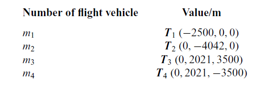
According to the configuration constraints described in the Section 2, the expected parameters of each sub-vehicle in the relative LOS coordinate system can be designed. Refer to Fig. 2, assuming that the coordinate vector of virtual leader is
 $\left( {0,0,0} \right)$
, and the coordinate vector of the first flight vehicle is
$\left( {0,0,0} \right)$
, and the coordinate vector of the first flight vehicle is
 ${m_1}\left( {{x_1},{y_1},{z_1}} \right)$
, while the remain three sub-vehicles are defined as
${m_1}\left( {{x_1},{y_1},{z_1}} \right)$
, while the remain three sub-vehicles are defined as
 ${m_2}\left( {{x_2},{y_2},{z_2}} \right),{m_3}\left( {{x_3},{y_3},{z_3}} \right),$
 ${m_4}\left( {{x_4},{y_4},{z_4}} \right)$
, respectively, and the related plane formed by them is defined as
${m_4}\left( {{x_4},{y_4},{z_4}} \right)$
, respectively, and the related plane formed by them is defined as
 ${T_2}{T_3}{T_4}$
. The vector connecting the
${T_2}{T_3}{T_4}$
. The vector connecting the
 ${1^{th}}$
flight vehicle and the target is defined as
${1^{th}}$
flight vehicle and the target is defined as
 $\overrightarrow {{T_1}T} $
, and the vector between the virtual leader and the
$\overrightarrow {{T_1}T} $
, and the vector between the virtual leader and the
 ${1^{th}}$
flight vehicle is
${1^{th}}$
flight vehicle is
 $\overrightarrow {{T_1}O} $
. Next there exists the following geometric relationship.
$\overrightarrow {{T_1}O} $
. Next there exists the following geometric relationship.
-
(1) The baseline length
${L_{23}},{L_{24}},{L_{34}}$
between each sub-vehicle(2)
\begin{align}\left\{ {\begin{array}{*{20}{l}}{\Delta {x_{32}} = {x_3} - {x_2},\Delta {x_{42}} = {x_4} - {x_2},\Delta {x_{43}} = {x_4} - {x_3}}\\[2pt]{\Delta {y_{32}} = {y_3} - {y_2},\Delta {y_{42}} = {y_4} - {y_2},\Delta {y_{43}} = {y_4} - {y_3}}\\[2pt]{\Delta {z_{32}} = {z_3} - {z_2},\Delta {z_{42}} = {z_4} - {z_2},\Delta {z_{43}} = {z_4} - {z_3}}\end{array}} \right.\end{align}
(3)
\begin{align}\left\{ {\begin{array}{*{20}{c}}{{L_{23}} = \sqrt {{{\left( {\Delta {y_{32}}} \right)}^2} + {{\left( {\Delta {z_{32}}} \right)}^2}} }\\[8pt]{{L_{24}} = \sqrt {{{\left( {\Delta {y_{42}}} \right)}^2} + {{\left( {\Delta {z_{42}}} \right)}^2}} }\\[8pt]{{L_{34}} = \sqrt {{{\left( {\Delta {y_{43}}} \right)}^2} + {{\left( {\Delta {z_{43}}} \right)}^2}} }\end{array}} \right.\end{align}


Table 1 Expected parameters of each flight vehicle
-
(2) The distance
${L_0}$
between the
${1^{th}}$
sub-vehicle and the plane
${T_2}{T_3}{T_4}$


 \begin{align}{L_0} = \frac{{{L_{0f}}}}{{{L_{0m}}}}\end{align}
where
 \begin{align*}{L_{0f}} &= \left| ({x_2} - {x_1})\left( {\Delta {z_{32}}\Delta {y_{42}} - \Delta {y_{32}}\Delta {z_{42}}} \right) + ({y_2} - {y_1})\left( {\Delta {x_{32}}\Delta {z_{42}} - \Delta {z_{32}}\Delta {x_{42}}} \right) \right.\\ & \left.+ ({z_2} - {z_1})\left( {\Delta {y_{32}}\Delta {x_{42}} - \Delta {x_{32}}\Delta {y_{42}}} \right) \right|,\\{L_{0m}} & = \sqrt {\!\left( {{{\left( {\Delta {y_{32}}\Delta {z_{42}} - \Delta {z_{32}}\Delta {y_{42}}} \right)}^2} + {{\left( {\Delta {z_{32}}\Delta {x_{42}} - \Delta {x_{32}}\Delta {z_{42}}} \right)}^2} + {{\left( {\Delta {x_{32}}\Delta {y_{42}} - \Delta {y_{32}}\Delta {x_{42}}} \right)}^2}} \right)}.\end{align*}
-
(3) The offset angle
$\Delta center$
between
$\overrightarrow {{T_1}T} $
and
$\overrightarrow {{T_1}O} $
(5)
\begin{align}\left\{ {\begin{array}{*{20}{c}}{\Delta x = \dfrac{{{x_2} + {x_3} + {x_4}}}{3} - {x_1}}\\[8pt]{\Delta y = \dfrac{{{y_2} + {y_3} + {y_4}}}{3} - {y_1}}\\[8pt]{\Delta z = \dfrac{{{z_2} + {z_3} + {z_4}}}{3} - {z_1}}\end{array}} \right.\end{align}
(6)
\begin{align}\Delta center = \arccos \left( {\frac{{\Delta x}}{{\sqrt {\Delta {x^2} + \Delta {y^2} + \Delta {z^2}} }}} \right)\end{align}


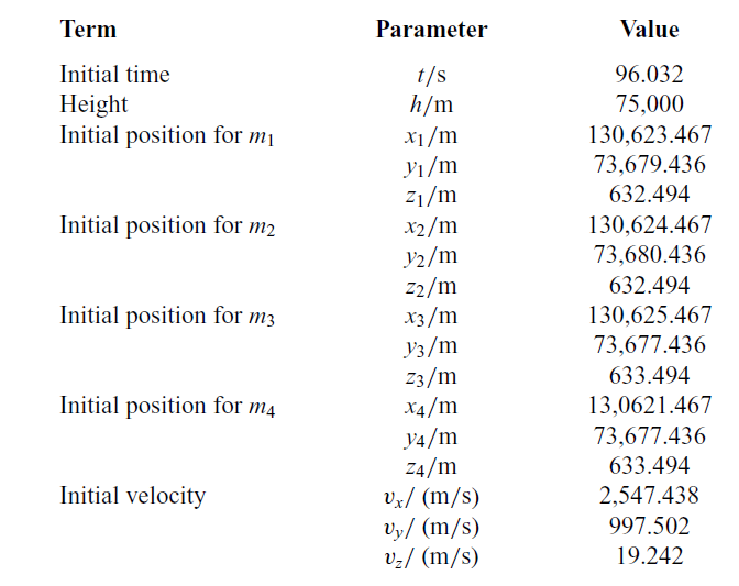
According to Equations (2)–(6), the expected coordinate vector of each sub-vehicle relative to the virtual leader in the LOS coordinate system can be designed, as shown in Table 1.
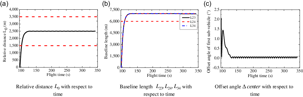
Whether these parameters shown in Table 1 meet the formation constraints described in the Section 2 or not, which can be judged by substituting them into Equations (2)–(6) yields
-
(a)
$\Delta center = {0^ \circ }$
, which stands for the
${1^{th}}$
flight vehicle is projected on the centre of the plane
${T_2}{T_3}{T_4}$
and thus meet the requirement of offset angle; -
(b)
${L_{23}},{L_{24}},{L_{34}}=7{\rm{km}}$
, which stands for the baseline length between each sub-vehicle is more than
$6{\rm{km}}$
; -
(c)
${L_0}=2.5{\rm{km}}$
, which means that the distance of the
${1^{th}}$
flight vehicle relative to the plane
${T_2}{T_3}{T_4}$
is between
$1.5$
and
$3.5{\rm{km}}$
.


In summary, the position parameters of each flight vehicle shown in Table 1 meet the configuration constraints described in the Section 2. Then the appropriate control law is designed in the Section 4 to control the four flight vehicles to fly to their expected positions and simulation verification is performed in the Section 5.
4.0 DESIGN OF CONTROL LAW
In this section, the control law is completely designed in the following three steps. The first is to design the NTSMC law with considering the external disturbances of the system; the second is design the second-order NTSMC law with considering the dynamic characteristic of the autopilot of flight vehicle; the third one is that a novel improved control law is proposed to guarantee the finite time convergence of the system errors, and also effectively suppress the small chattering phenomenon of the sliding mode surfaces and the acceleration responses.
4.1 Design of NTSMC law
For system (1), define the flight error vector and velocity error vector of each sub-vehicle in the LOS coordinate system as
 \begin{align}\begin{array}{l}{{\textbf{\textit{e}}}_{{\textbf{1}}{\textbf{\textit{,i}}}}} = {{\textbf{\textit{x}}}_{{\textbf{\textit{s,i}}}}} - {{\textbf{\textit{x}}}_{{\textbf{\textit{q,i}}}}}\\[3pt]{{\textbf{\textit{e}}}_{{\textbf{2}}{\textbf{\textit{,i}}}}} = {{\textbf{\textit{v}}}_{{\textbf{\textit{s,i}}}}}\end{array}\end{align}
Differentiating Equation (7) with respect to time can be obtained as
 \begin{align}\begin{array}{l}{{{\dot{\textbf{\textit{e}}}}}_{{\textbf{1}}{\textbf{\textit{,i}}}}} = {{\textbf{\textit{e}}}_{{\textbf{2}}{\textbf{\textit{,i}}}}}\\[3pt]{{{\dot{\textbf{\textit{e}}}}}_{{\textbf{2}}{\textbf{\textit{,i}}}}} = {{\textbf{\textit{a}}}_{{\textbf{\textit{s,i}}}}}\left( {\textbf{\textit{t}}} \right) + {{\textbf{\textit{d}}}_{\textbf{\textit{s}}}}\left( {\textbf{\textit{t}}} \right)\end{array}\end{align}
For system (8), take any sub-vehicle as an example, and choose the NTSM as
 \begin{align}{{\textbf{\textit{s}}}} = {{\textbf{\textit{e}}}_{\textbf{1}}} + \beta si{g^\gamma }\left( {{{\textbf{\textit{e}}}_{\textbf{2}}}} \right)\end{align}
where
 $\beta >0,1 < \gamma <2,si{g^\gamma }\left( {{{{\textbf{\textit{e}}}}_{\textbf{2}}}} \right) = {\left| {{{{\textbf{\textit{e}}}}_{\textbf{2}}}} \right|^\gamma }{\mathop{\rm sgn}} \left( {{{{\textbf{\textit{e}}}}_{\textbf{2}}}} \right)$
, is the sign function.
$\beta >0,1 < \gamma <2,si{g^\gamma }\left( {{{{\textbf{\textit{e}}}}_{\textbf{2}}}} \right) = {\left| {{{{\textbf{\textit{e}}}}_{\textbf{2}}}} \right|^\gamma }{\mathop{\rm sgn}} \left( {{{{\textbf{\textit{e}}}}_{\textbf{2}}}} \right)$
, is the sign function.
Differentiating Equation (9) with respect to time yields
 \begin{align}{\dot{\textbf{\textit{s}}}} &= {{{\dot{\textbf{\textit{e}}}}}_{\textbf{1}}} + \beta \gamma {\left| {{{\textbf{\textit{e}}}_{\textbf{2}}}} \right|^{\gamma - 1}}{{{\dot{\textbf{\textit{e}}}}}_{\textbf{2}}}\nonumber\\[3pt] &= {{\textbf{\textit{e}}}_{\textbf{2}}} + \beta \gamma {\left| {{{\textbf{\textit{e}}}_{\textbf{2}}}} \right|^{\gamma - 1}}\left( {{{\textbf{\textit{a}}}_{\textbf{\textit{s}}}} + {{\textbf{\textit{d}}}_{\textbf{\textit{s}}}}\left( {\textbf{\textit{t}}} \right)} \right)\end{align}
Choose the fast terminal sliding mode reaching law as
 \begin{align}{\dot{\textbf{\textit{s}}}} = - {k_1}{\textbf{\textit{s}}} - {k_2}si{g^\rho }\left( {\textbf{\textit{s}}} \right)\end{align}
where
 ${k_1}>0,{k_2}>0,0 < \rho <1$
. Compare Equations (10) and (11), the adaptive NTSMC law can be obtained as
${k_1}>0,{k_2}>0,0 < \rho <1$
. Compare Equations (10) and (11), the adaptive NTSMC law can be obtained as
 \begin{align}{{\textbf{\textit{a}}}_{\textbf{\textit{s}}}} = - \frac{{si{g^{2 - \gamma }}\left( {{{\textbf{\textit{e}}}_{\textbf{2}}}} \right)}}{{\beta \gamma }} - {k_1}{\textbf{\textit{s}}} - {k_2}si{g^\rho }\left( {\textbf{\textit{s}}} \right) - \varepsilon {\mathop{\rm sgn}} \left( {\textbf{\textit{s}}} \right)\end{align}
where
 $\varepsilon {\mathop{\rm sgn}} \left( {\textbf{\textit{s}}} \right)$
is used to compensate the external disturbance. if
$\varepsilon {\mathop{\rm sgn}} \left( {\textbf{\textit{s}}} \right)$
is used to compensate the external disturbance. if
 $\varepsilon $
is too large, the control variable
$\varepsilon $
is too large, the control variable
 ${{\textbf{\textit{a}}}_{\textbf{\textit{s}}}}$
will be too large; However, if
${{\textbf{\textit{a}}}_{\textbf{\textit{s}}}}$
will be too large; However, if
 $\varepsilon $
is too small, it will easily cause system instability. Define
$\varepsilon $
is too small, it will easily cause system instability. Define
 $\tilde \delta = \delta - \hat \delta $
, in which
$\tilde \delta = \delta - \hat \delta $
, in which
 $\hat \delta $
is the estimated value of the variable
$\hat \delta $
is the estimated value of the variable
 $\delta $
. Assume that there exists
$\delta $
. Assume that there exists
 $\left| {\tilde \delta } \right| < {\varepsilon _1}$
for any kinds of disturbance, and
$\left| {\tilde \delta } \right| < {\varepsilon _1}$
for any kinds of disturbance, and
 ${\varepsilon _1}$
is a small normal number. Then the adaptive gain
${\varepsilon _1}$
is a small normal number. Then the adaptive gain
 $\varepsilon $
in Equation (12) can be designed as
$\varepsilon $
in Equation (12) can be designed as
 \begin{align}\varepsilon = \hat \delta + {\varepsilon _1},\dot \hat \delta = \lambda \beta \gamma {\left| {{{\textbf{\textit{e}}}_{\textbf{2}}}} \right|^{\gamma - 1}}\left| {\textbf{\textit{s}}} \right|\end{align}
where
 $\lambda >0$
is the weighting coefficient to be designed.
$\lambda >0$
is the weighting coefficient to be designed.
Theorem 1. For system (8) and sliding mode (9), the control law (12) can guarantee that the formation system controlling errors converges to zero in a finite time.
Proof of Theorem 1: Substituting Equation (12) into Equation (10) yields
 \begin{align}{\dot{\textbf{\textit{s}}}} = \beta \gamma {\left| {{{\textbf{\textit{e}}}_{\textbf{2}}}} \right|^{\gamma - 1}}\left( { - {k_1}{\textbf{\textit{s}}} - {k_2}si{g^\rho }\left( {\textbf{\textit{s}}} \right)} \right) + {{\textbf{\textit{d}}}_{\textbf{\textit{s}}}}\left( {\textbf{\textit{t}}} \right) - \varepsilon {\mathop{\rm sgn}} \left( {\textbf{\textit{s}}} \right)\end{align}
Define the following Lyapunov function
 \begin{align}{\textbf{\textit{V}}} = \frac{1}{2}{{\textbf{\textit{s}}}^2} + \frac{1}{{2\lambda }}{\tilde \delta ^2}\end{align}
Differentiating Equation (15) with respect to time yields
 \begin{align}{\dot{\textbf{\textit{V}}}} &= {\dot{\textbf{\textit{s}}}} + \frac{1}{\lambda }\tilde \delta \dot{\tilde{\delta}} \nonumber\\[3pt] &= \beta \gamma {\left| {{{\textbf{\textit{e}}}_{\textbf{2}}}} \right|^{\gamma - 1}}{\textbf{\textit{s}}}\left( { - {k_1}{\textbf{\textit{s}}} - {k_2}si{g^\rho }\left( {\textbf{\textit{s}}} \right) + {{\textbf{\textit{d}}}_{\textbf{\textit{s}}}}\left( {\textbf{\textit{t}}} \right) - \varepsilon {\mathop{\rm sgn}} \left( {\textbf{\textit{s}}} \right)} \right) + \frac{1}{\lambda }\tilde \delta \left( {\dot{\tilde{\delta}} - \dot{\hat{\delta}} } \right)\nonumber\\[3pt] &\le \beta \gamma {\left| {{{\textbf{\textit{e}}}_{\textbf{2}}}} \right|^{\gamma - 1}}\left( { - {k_1}{{\textbf{\textit{s}}}^2} - {k_2}{{\left| {\textbf{\textit{s}}} \right|}^{\rho +1}} + \delta \left| {\textbf{\textit{s}}} \right| - {\varepsilon _1}\left| {\textbf{\textit{s}}} \right| - \hat \delta \left| {\textbf{\textit{s}}} \right|} \right) - \frac{1}{\lambda }\tilde \delta \dot{\hat{\delta}} \end{align}
Substituting Equation (13) into Equation (16) yields
 \begin{align} &{\dot{\textbf{\textit{V}}}} \le \beta \gamma {\left| {{{\textbf{\textit{e}}}_{\textbf{2}}}} \right|^{\gamma - 1}}\left( { - {k_1}{{\textbf{\textit{s}}}^2} - {k_2}{{\left| {\textbf{\textit{s}}} \right|}^{\rho +1}} + \delta \left| {\textbf{\textit{s}}} \right| - {\varepsilon _1}\left| {\textbf{\textit{s}}} \right| - \hat \delta \left| {\textbf{\textit{s}}} \right|} \right) - \tilde \delta \beta \gamma {\left| {{{\textbf{\textit{e}}}_{\textbf{2}}}} \right|^{\gamma - 1}}\left| {\textbf{\textit{s}}} \right|\nonumber\\[3pt] &\quad \le \beta \gamma {\left| {{{\textbf{\textit{e}}}_{\textbf{2}}}} \right|^{\gamma - 1}}\left( { - {k_1}{{\textbf{\textit{s}}}^2} - {k_2}{{\left| {\textbf{\textit{s}}} \right|}^{\rho +1}} - {\varepsilon _1}\left| {\textbf{\textit{s}}} \right|} \right)\nonumber\\ &\le 0\end{align}
Lemma 1 Lemma 1 (Reference Yu, Yu and Shirinzadeh22). Consider the nonlinear system
 $\dot x = f\left( {x,t} \right),x \in {R^n}$
, and if there exists a positive defined Lyapunov function
$\dot x = f\left( {x,t} \right),x \in {R^n}$
, and if there exists a positive defined Lyapunov function
 $V\left( x \right)$
and the parameters
$V\left( x \right)$
and the parameters
 ${\beta _1}>0,{\beta _3}>0$
and
${\beta _1}>0,{\beta _3}>0$
and
 ${\beta _2} \in \left( {0,1} \right)$
satisfy
${\beta _2} \in \left( {0,1} \right)$
satisfy
 \begin{align}\dot V\left( t \right) + {\beta _3}V\left( t \right) + {\beta _1}{V^{{\beta _2}}}\left( t \right) \le 0\end{align}
Then the system state can reach zero in a finite time
 ${T_{reach}}$
, which is given by
${T_{reach}}$
, which is given by
 \begin{align}{T_{reach}} \le \frac{1}{{{\beta _3}\left( {1 - {\beta _2}} \right)}}\ln \frac{{{\beta _3}{V^{1 - {\beta _2}}}\left( {{t_0}} \right) + {\beta _1}}}{{{\beta _1}}}\end{align}
where
 $V\left( {{x_0}} \right)$
is the initial value of
$V\left( {{x_0}} \right)$
is the initial value of
 $V\left( x \right)$
.
$V\left( x \right)$
.
According to Lemma 1, since
 ${\varepsilon _1}$
is a small normal number, the system (8) can converge to the sliding mode surface; When
${\varepsilon _1}$
is a small normal number, the system (8) can converge to the sliding mode surface; When
 ${{\textbf{\textit{e}}}_{\textbf{2}}}=0$
and
${{\textbf{\textit{e}}}_{\textbf{2}}}=0$
and
 $\textbf{\textit{s}} \ne 0$
, the sliding mode surface (9) shows that
$\textbf{\textit{s}} \ne 0$
, the sliding mode surface (9) shows that
 ${{\textbf{\textit{e}}}_{\textbf{1}}} \ne 0$
, which means that the system do not reach the stable state, and thus
${{\textbf{\textit{e}}}_{\textbf{1}}} \ne 0$
, which means that the system do not reach the stable state, and thus
 $\dot{\textbf{\textit{V}}}$
is not equal to zero, that is,
$\dot{\textbf{\textit{V}}}$
is not equal to zero, that is,
 $\dot{\textbf{\textit{V}}} < 0$
at the current time. From Equations (16) and (17), it is obvious that the system will converge to zero in a finite time in this case; when the sliding mode surface
$\dot{\textbf{\textit{V}}} < 0$
at the current time. From Equations (16) and (17), it is obvious that the system will converge to zero in a finite time in this case; when the sliding mode surface
 $\textbf{\textit{s}} = 0$
, it indicates that the system state vectors
$\textbf{\textit{s}} = 0$
, it indicates that the system state vectors
 ${{\textbf{\textit{e}}}_{\textbf{1}}}$
and
${{\textbf{\textit{e}}}_{\textbf{1}}}$
and
 ${{\textbf{\textit{e}}}_{\textbf{2}}}$
reach the equilibrium point, that is, each sub-vehicle flies to the desired terminal position, and the velocity relative to the virtual leader is
${{\textbf{\textit{e}}}_{\textbf{2}}}$
reach the equilibrium point, that is, each sub-vehicle flies to the desired terminal position, and the velocity relative to the virtual leader is
 $0{\rm{m/s}}$
.
$0{\rm{m/s}}$
.
Here the Proof of Theorem 1 is completed.
4.2 Design of control law considering the dynamic characteristic of autopilot
Based on Section 4.1, further considering the first-order dynamic characteristic of the autopilot, and then the adaptive second-order sliding mode control (SOSMC) law with finite time convergence is designed. The first-order dynamic characteristic of the autopilot can be expressed as
 \begin{align}{{\dot{\textbf{\textit{a}}}}_{{\textbf{\textit{m,i}}}}} = - \frac{1}{\tau }{{\textbf{\textit{a}}}_{{\textbf{\textit{m,i}}}}} + \frac{1}{\tau }{{\textbf{\textit{u}}}_{\textbf{\textit{i}}}}\end{align}
where
 $\tau $
is the delay time constant of autopilot;
$\tau $
is the delay time constant of autopilot;
 ${{\textbf{\textit{u}}}_{\textbf{\textit{i}}}} = {{\textbf{\textit{a}}}_{{\textbf{\textit{s,i}}}}}$
is acceleration command vector;
${{\textbf{\textit{u}}}_{\textbf{\textit{i}}}} = {{\textbf{\textit{a}}}_{{\textbf{\textit{s,i}}}}}$
is acceleration command vector;
 ${{\textbf{\textit{a}}}_{{\textbf{\textit{m,i}}}}}$
is the acceleration vector in the LOS coordinate system.
${{\textbf{\textit{a}}}_{{\textbf{\textit{m,i}}}}}$
is the acceleration vector in the LOS coordinate system.
Combine with Equation (20), the system (8) can be further rewritten as
 \begin{align}{{{\dot{\textbf{\textit{e}}}}}_{{\textbf{1}}{\textbf{\textit{,i}}}}} &= {{\textbf{\textit{e}}}_{{\textbf{2}}{\textbf{\textit{,i}}}}}\nonumber\\[3pt]{{{\dot{\textbf{\textit{e}}}}}_{{\textbf{2}}{\textbf{\textit{,i}}}}} &= {{\textbf{\textit{e}}}_{{\textbf{3}}{\textbf{\textit{,i}}}}}\nonumber\\[3pt] {{{\dot{\textbf{\textit{e}}}}}_{{\textbf{3}}{\textbf{\textit{,i}}}}} &= - \frac{1}{\tau }{{\textbf{\textit{a}}}_{{\textbf{\textit{m,i}}}}} + \frac{1}{\tau }{{\textbf{\textit{u}}}_{\textbf{\textit{i}}}} + {{\textbf{\textit{d}}}_{\textbf{\textit{s}}}}\left( {\textbf{\textit{t}}} \right)\end{align}
For Equation (21), choose the linear sliding mode surface as
 \begin{align}{{\textbf{\textit{s}}}_{\textbf{1}}} = {k_0}{{\textbf{\textit{e}}}_{\textbf{1}}} + {{\textbf{\textit{e}}}_{\textbf{2}}}\end{align}
where
 ${k_0}>0$
is the control parameter to be designed.
${k_0}>0$
is the control parameter to be designed.
Differentiating Equation (22) with respect to time once and twice respectively yields
 \begin{align}{{{\dot{\textbf{\textit{s}}}}}_{\textbf{1}}} &= {k_0}{{\dot{\textbf{\textit{e}}}}_{\textbf{1}}} + {{\dot{\textbf{\textit{e}}}}_{\textbf{2}}}\nonumber\\[3pt] &= {k_0}{{\textbf{\textit{e}}}_{\textbf{2}}} + {{\textbf{\textit{e}}}_{\textbf{3}}}\end{align}
 \begin{align}{{{\ddot{\textbf{\textit{s}}}}}_{\textbf{1}}} &= {k_0}{{{\dot{\textbf{\textit{e}}}}}_{\textbf{2}}} + {{{\dot{\textbf{\textit{e}}}}}_{\rm{3}}}\nonumber\\ &= {k_0}{{{\textbf{\textit{e}}}}_{\rm{3}}} + {{{\dot{\textbf{\textit{e}}}}}_{\rm{3}}}\nonumber\\ &= {k_0}{{{\textbf{\textit{e}}}}_{\rm{3}}} - \frac{1}{\tau }{{{\textbf{\textit{a}}}}_{{{\textbf{\textit{m,i}}}}}} + \frac{1}{\tau }{{{\textbf{\textit{u}}}}_{{\textbf{\textit{i}}}}} + {{{\textbf{\textit{d}}}}_{{\textbf{\textit{s}}}}}\left( {{\textbf{\textit{t}}}} \right)\end{align}
To assure that the flight state errors of these four flight vehicles converge quickly in a finite time, then take
 ${{{\textbf{\textit{s}}}}_{\textbf{1}}}$
and
${{{\textbf{\textit{s}}}}_{\textbf{1}}}$
and
 ${{\dot{\textbf{\textit{s}}}}_{\textbf{1}}}$
as state variables, and choose the following non-singular terminal sliding mode as
${{\dot{\textbf{\textit{s}}}}_{\textbf{1}}}$
as state variables, and choose the following non-singular terminal sliding mode as
 \begin{align}{{{\textbf{\textit{s}}}}_{\textbf{2}}} = {{{\textbf{\textit{s}}}}_{\textbf{1}}} + \beta si{g^\gamma }\left( {{{{\dot{\textbf{\textit{s}}}}}_{\textbf{1}}}} \right)\end{align}
where
 $si{g^\gamma }\left( {{{{\dot{\textbf{\textit{s}}}}}_{\textbf{1}}}} \right) = {\left| {{{{\dot{\textbf{\textit{s}}}}}_{\textbf{1}}}} \right|^\gamma }{\mathop{\rm sgn}} \left( {{{{\dot{\textbf{\textit{s}}}}}_{\textbf{1}}}} \right)$
, and the other parameters are consistent with Equation (9). Differentiating Equation (25) yields
$si{g^\gamma }\left( {{{{\dot{\textbf{\textit{s}}}}}_{\textbf{1}}}} \right) = {\left| {{{{\dot{\textbf{\textit{s}}}}}_{\textbf{1}}}} \right|^\gamma }{\mathop{\rm sgn}} \left( {{{{\dot{\textbf{\textit{s}}}}}_{\textbf{1}}}} \right)$
, and the other parameters are consistent with Equation (9). Differentiating Equation (25) yields
 \begin{align}{{{\dot{\textbf{\textit{s}}}}}_{\textbf{2}}} &= {{{\dot{\textbf{\textit{s}}}}}_{\textbf{1}}} + \beta \gamma {\left| {{{{\dot{\textbf{\textit{s}}}}}_{\textbf{1}}}} \right|^{\gamma - 1}}{{{\ddot{\textbf{\textit{s}}}}}_{\textbf{1}}}\nonumber\\[3pt] &= {{{\dot{\textbf{\textit{s}}}}}_{\textbf{1}}} + \beta \gamma {\left| {{{{\dot{\textbf{\textit{s}}}}}_{\textbf{1}}}} \right|^{\gamma - 1}}\left( {{k_0}{{{\textbf{\textit{e}}}}_{\rm{3}}} - \frac{1}{\tau }{{{\textbf{\textit{a}}}}_{{{\textbf{\textit{m,i}}}}}} + \frac{1}{\tau }{{{\textbf{\textit{u}}}}_{{\textbf{\textit{i}}}}} + {{{\textbf{\textit{d}}}}_{{\textbf{\textit{s}}}}}\left( {{\textbf{\textit{t}}}} \right)} \right)\end{align}
Similarly, in this case, the control law can be obtained as
 \begin{align}{{{\textbf{\textit{u}}}}_{{\textbf{\textit{i}}}}} = - \frac{\tau }{{\beta \gamma }}{\left| {{{{\dot{\textbf{\textit{s}}}}}_{\textbf{1}}}} \right|^{2 - \gamma }}{\mathop{\rm sgn}} \left( {{{{\dot{\textbf{\textit{s}}}}}_{\textbf{1}}}} \right) - \frac{\tau }{{\beta \gamma }}{\left| {{{{\dot{\textbf{\textit{s}}}}}_{\textbf{1}}}} \right|^{1 - \gamma }}\left[ {{k_1}{{{\textbf{\textit{s}}}}_{\textbf{2}}} + {k_2}si{g^\rho }\left( {{{{\textbf{\textit{s}}}}_{\textbf{2}}}} \right)} \right] - \left( {\tau {k_0} - 1} \right){{{\textbf{\textit{e}}}}_{\rm{3}}} - \tau {{{\textbf{\textit{d}}}}_{{\textbf{\textit{s}}}}}\left( {{\textbf{\textit{t}}}} \right)\end{align}
To avoid
 $\frac{\tau }{{\beta \gamma }}{\left| {{{{\dot{\textbf{\textit{s}}}}}_{\textbf{1}}}} \right|^{1 - \gamma }}$
occurs singularity when
$\frac{\tau }{{\beta \gamma }}{\left| {{{{\dot{\textbf{\textit{s}}}}}_{\textbf{1}}}} \right|^{1 - \gamma }}$
occurs singularity when
 ${{\dot{\textbf{\textit{s}}}}_{\textbf{1}}} \to 0$
, Equation (27) can be simplified as
${{\dot{\textbf{\textit{s}}}}_{\textbf{1}}} \to 0$
, Equation (27) can be simplified as
 \begin{align}{{{\textbf{\textit{u}}}}_{{\textbf{\textit{i}}}}} = - \frac{\tau }{{\beta \gamma }}{\left| {{{{\dot{\textbf{\textit{s}}}}}_{\textbf{1}}}} \right|^{2 - \gamma }}{\mathop{\rm sgn}} \left( {{{{\dot{\textbf{\textit{s}}}}}_{\textbf{1}}}} \right) - \tau \left[ {{k_1}{{{\textbf{\textit{s}}}}_{\textbf{2}}} + {k_2}si{g^\rho }\left( {{{{\textbf{\textit{s}}}}_{\textbf{2}}}} \right)} \right] - \left( {\tau {k_0} - 1} \right){{{\textbf{\textit{e}}}}_{\rm{3}}} - \tau {{{\textbf{\textit{d}}}}_{{\textbf{\textit{s}}}}}\left( {{\textbf{\textit{t}}}} \right)\end{align}
Therefore, according to Equation (28), the adaptive NTSMC law with considering the first-order dynamic characteristic of the autopilot can be written as
 \begin{align}{{{\textbf{\textit{u}}}}_{{\textbf{\textit{i}}}}} = - \frac{\tau }{{\beta \gamma }}{\left| {{{{\dot{\textbf{\textit{s}}}}}_{\textbf{1}}}} \right|^{2 - \gamma }}{\mathop{\rm sgn}} \left( {{{{\dot{\textbf{\textit{s}}}}}_{\textbf{1}}}} \right) - \tau \left[ {{k_1}{{{\textbf{\textit{s}}}}_{\textbf{2}}} + {k_2}si{g^\rho }\left( {{{{\textbf{\textit{s}}}}_{\textbf{2}}}} \right)} \right] - \left( {\tau {k_0} - 1} \right){{{\textbf{\textit{e}}}}_{\rm{3}}} - \tau \varepsilon {\mathop{\rm sgn}} \left( {{{{\textbf{\textit{s}}}}_{\textbf{2}}}} \right)\end{align}
where the adaptive gain
 $\varepsilon $
in Equation (29) can be taken as
$\varepsilon $
in Equation (29) can be taken as
 \begin{align}\varepsilon = \hat \delta + {\varepsilon _1},\dot{\hat{\delta}} = \tau \lambda \beta \gamma {\left| {{{{\textbf{\textit{e}}}}_{\textbf{2}}}} \right|^{\gamma - 1}}\left| {{{{\textbf{\textit{s}}}}_{\textbf{2}}}} \right|\end{align}
The proof and related discussion of stability is similar to the Section 4.1.
4.3 A novel control law
In Section 4.2, the second-order sliding control law is designed, which ensure that the formation configuration of the system converges in a finite time; however, this control algorithm will result in the small-amplitude chattering phenomenon of the sliding mode surfaces and control variables at the equilibrium point. Hence, in this section, a novel improved control law is proposed, which makes the sliding mode surfaces asymptotically converge to zero without crossing the zero point. Meanwhile, the chattering of acceleration responses is effectively eliminated, and the robustness of the system is subsequently enhanced.
Define the sliding mode function of any sub-vehicle as
 \begin{align}{{{\textbf{\textit{s}}}}_1} = {{\textbf{\textit{y}}}}\left( {{\textbf{\textit{x}}}} \right)=0\end{align}
For Equation (31), the first-order differential equation and second-order differential equation can be expressed as
 \begin{align}{{\dot{\textbf{\textit{s}}}}_1}{\bf{ = h}}\left( {{\textbf{\textit{x}}}} \right)\end{align}
 \begin{align}{{\ddot{\textbf{\textit{s}}}}_1} = {{\textbf{\textit{f}}}}\left( {{\textbf{\textit{x}}}} \right) + {{\textbf{\textit{b}}}}\left( {{\textbf{\textit{x}}}} \right){{\textbf{\textit{u}}}}\end{align}
For Equations (32) and (33), in which
 ${{\textbf{\textit{h}}}}\left( {{\textbf{\textit{x}}}} \right),{{\textbf{\textit{f}}}}\left( {{\textbf{\textit{x}}}} \right),{{\textbf{\textit{b}}}}\left( {{\textbf{\textit{x}}}} \right)$
are the known functions relating to the system.
${{\textbf{\textit{h}}}}\left( {{\textbf{\textit{x}}}} \right),{{\textbf{\textit{f}}}}\left( {{\textbf{\textit{x}}}} \right),{{\textbf{\textit{b}}}}\left( {{\textbf{\textit{x}}}} \right)$
are the known functions relating to the system.
For the sliding function (31) and the first-order differential equation (32), which need to converge to zero at the given time
 ${t_r}$
, and define the following Lyapunov function as
${t_r}$
, and define the following Lyapunov function as
 \begin{align}{{{\textbf{\textit{V}}}}_1} = \frac{1}{2}{{{\textbf{\textit{s}}}}_1}^2\end{align}
Differentiating Equation (34) with respect to time yields
 \begin{align}{{\dot{\textbf{\textit{V}}}}_1} = {{{\textbf{\textit{s}}}}_1}{{\dot{\textbf{\textit{s}}}}_1}\end{align}
To assure that the sliding mode surface (31) converges to zero in a finite time, that is
 ${{\dot{\textbf{\textit{V}}}}_{\textbf{1}}} \le 0$
, and thus design
${{\dot{\textbf{\textit{V}}}}_{\textbf{1}}} \le 0$
, and thus design
 ${{\dot{\textbf{\textit{s}}}}_1}$
as
${{\dot{\textbf{\textit{s}}}}_1}$
as
 \begin{align}{{\dot{\textbf{\textit{s}}}}_1} = - \frac{{{\mathop{\rm n}\nolimits} {{{\textbf{\textit{s}}}}_1}}}{{{{\mathop{\rm t}\nolimits} _r} - {\mathop{\rm t}\nolimits} }},{\mathop{\rm n}\nolimits} >1\end{align}
where
 ${\mathop{\rm n}\nolimits} >1$
is the coefficient to be designed. Substituting Equation (36) into Equation (35) yields
${\mathop{\rm n}\nolimits} >1$
is the coefficient to be designed. Substituting Equation (36) into Equation (35) yields
 \begin{align}{{\dot{\textbf{\textit{V}}}}_1} = - \frac{{{\mathop{\rm n}\nolimits} {{{\textbf{\textit{s}}}}_1}^2}}{{{{\mathop{\rm t}\nolimits} _r} - {\mathop{\rm t}\nolimits} }}\end{align}
Substituting Equation (34) into Equation (37) yields
 \begin{align}{{\dot{\textbf{\textit{V}}}}_1} = - \frac{{2{\rm{n}}{{{\textbf{\textit{V}}}}_1}}}{{{{\rm{t}}_{\rm{r}}} - {\rm{t}}}}\end{align}
Integrating Equation (38) yields
 \begin{align}\int_{{t_0}}^t {{{{\dot{\textbf{\textit{V}}}}}_{\textbf{1}}}\left( t \right)dt = {{{\textbf{\textit{V}}}}_{\textbf{1}}}\left( t \right) = \frac{{{{{\textbf{\textit{V}}}}_{\textbf{1}}}\left( {{t_0}} \right)}}{{{{\left( {{t_r} - {t_0}} \right)}^{2n}}}}{{\left( {{t_r} - t} \right)}^{2n}}} \end{align}
where
 $\mathop {\lim }\limits_{t \to {t_r}} {\left( {{t_r} - t} \right)^{2n}}$
is equal to zero when
$\mathop {\lim }\limits_{t \to {t_r}} {\left( {{t_r} - t} \right)^{2n}}$
is equal to zero when
 $n>0.5$
, and thus the Lyapunov function
$n>0.5$
, and thus the Lyapunov function
 ${{{\textbf{\textit{V}}}}_{\textbf{1}}}\left( t \right)$
can converge to zero within the desired time
${{{\textbf{\textit{V}}}}_{\textbf{1}}}\left( t \right)$
can converge to zero within the desired time
 ${t_r}$
and the sliding mode surface
${t_r}$
and the sliding mode surface
 ${{{\textbf{\textit{s}}}}_1}$
can also reach zero at the same time(Reference Harl and Balakrishnan23). For the first-order derivative
${{{\textbf{\textit{s}}}}_1}$
can also reach zero at the same time(Reference Harl and Balakrishnan23). For the first-order derivative
 ${{\dot{\textbf{\textit{s}}}}_1}$
of the sliding mode surface, it can converge to zero within the designed time
${{\dot{\textbf{\textit{s}}}}_1}$
of the sliding mode surface, it can converge to zero within the designed time
 ${t_r}$
only when
${t_r}$
only when
 $n>1$
. Due to the initial value of
$n>1$
. Due to the initial value of
 ${{\dot{\textbf{\textit{s}}}}_1}$
totally depend on the initial conditions of the problem, thus
${{\dot{\textbf{\textit{s}}}}_1}$
totally depend on the initial conditions of the problem, thus
 ${{\dot{\textbf{\textit{s}}}}_1}$
may not meet the expected trajectory given by Equation (36) at the initial stage. Therefore, the control command needs to be able to make
${{\dot{\textbf{\textit{s}}}}_1}$
may not meet the expected trajectory given by Equation (36) at the initial stage. Therefore, the control command needs to be able to make
 ${{\dot{\textbf{\textit{s}}}}_1}$
reach the trajectory shown in Equation (36) within a limited time. Under this circumstance, define a new sliding mode surface as
${{\dot{\textbf{\textit{s}}}}_1}$
reach the trajectory shown in Equation (36) within a limited time. Under this circumstance, define a new sliding mode surface as
 \begin{align}{{{\textbf{\textit{s}}}}_2} = {{\dot{\textbf{\textit{s}}}}_1} + \frac{{{\mathop{\rm n}\nolimits} {{{\textbf{\textit{s}}}}_1}}}{{{{\mathop{\rm t}\nolimits} _r} - {\mathop{\rm t}\nolimits} }}\end{align}
Differentiating Equation (40) with respect to time yields
 \begin{align}{{{\dot{\textbf{\textit{s}}}}}_2} &= {{{\ddot{\textbf{\textit{s}}}}}_1} + \frac{{{\mathop{\rm n}\nolimits} {{{\dot{\textbf{\textit{s}}}}}_1}\left( {{{\mathop{\rm t}\nolimits} _r} - {\mathop{\rm t}\nolimits} } \right) + {\mathop{\rm n}\nolimits} {{{\textbf{\textit{s}}}}_1}}}{{{{\left( {{{\mathop{\rm t}\nolimits} _r} - {\mathop{\rm t}\nolimits} } \right)}^2}}}\nonumber\\[3pt] &= {{\textbf{\textit{f}}}}\left( {{\textbf{\textit{x}}}} \right) + \frac{{{\mathop{\rm n}\nolimits} {{{\dot{\textbf{\textit{s}}}}}_1}\left( {{{\mathop{\rm t}\nolimits} _r} - {\mathop{\rm t}\nolimits} } \right) + {\mathop{\rm n}\nolimits} {{{\textbf{\textit{s}}}}_1}}}{{{{\left( {{{\mathop{\rm t}\nolimits} _r} - {\mathop{\rm t}\nolimits} } \right)}^2}}} + {{\textbf{\textit{b}}}}\left( {{\textbf{\textit{x}}}} \right){{\textbf{\textit{u}}}}\end{align}
Define the following Lyapunov function as
 \begin{align}{{{\textbf{\textit{V}}}}_2} = \frac{1}{2}{{{\textbf{\textit{s}}}}_2}^2\end{align}
Differentiating Equation (42) with respect to time yields
 \begin{align}{{\dot{\textbf{\textit{V}}}}_2} = {{{\textbf{\textit{s}}}}_2}{{\dot{\textbf{\textit{s}}}}_2} = {{{\textbf{\textit{s}}}}_2}\left[ {{{\textbf{\textit{f}}}}\left( {{\textbf{\textit{x}}}} \right) + \frac{{{\mathop{\rm n}\nolimits} {{{\dot{\textbf{\textit{s}}}}}_1}\left( {{{\mathop{\rm t}\nolimits} _r} - t} \right) + {\mathop{\rm n}\nolimits} {{{\textbf{\textit{s}}}}_1}}}{{{{\left( {{{\mathop{\rm t}\nolimits} _r} - {\mathop{\rm t}\nolimits} } \right)}^2}}} + {{\textbf{\textit{b}}}}\left( {{\textbf{\textit{x}}}} \right){{\textbf{\textit{u}}}}} \right]\end{align}
To guarantee that
 ${{{\textbf{\textit{V}}}}_2}$
converges to zero in a finite time, and then the control command can be designed as
${{{\textbf{\textit{V}}}}_2}$
converges to zero in a finite time, and then the control command can be designed as
 \begin{align}{{\textbf{\textit{u}}}} = - \frac{1}{{{{\textbf{\textit{b}}}}\left( {{\textbf{\textit{x}}}} \right)}}\left( {{{\textbf{\textit{f}}}}\left( {{\textbf{\textit{x}}}} \right) + \frac{{{\mathop{\rm n}\nolimits} {{{\dot{\textbf{\textit{s}}}}}_1}\left( {{{\mathop{\rm t}\nolimits} _r} - {\mathop{\rm t}\nolimits} } \right) + {\mathop{\rm n}\nolimits} {{{\textbf{\textit{s}}}}_1}}}{{{{\left( {{{\mathop{\rm t}\nolimits} _r} - {\mathop{\rm t}\nolimits} } \right)}^2}}} + \eta {\rm{sgn}}\left( {{{{\dot{\textbf{\textit{s}}}}}_1} + \frac{{{\mathop{\rm n}\nolimits} {{{\textbf{\textit{s}}}}_1}}}{{{{\mathop{\rm t}\nolimits} _r} - {\mathop{\rm t}\nolimits} }}} \right)} \right)\end{align}
where
 $\eta >0$
is the control coefficient to be designed, which can affect the convergence speed of the system; substituting Equation (44) into Equation (43) yields
$\eta >0$
is the control coefficient to be designed, which can affect the convergence speed of the system; substituting Equation (44) into Equation (43) yields
 \begin{align}{{\dot{\textbf{\textit{V}}}}_2} < - \eta \left| {{{{\textbf{\textit{s}}}}_2}} \right| \le 0,{\kern 1pt} {\kern 1pt} {\kern 1pt} {\kern 1pt} {\kern 1pt} {\kern 1pt} {\kern 1pt} {\kern 1pt} {\kern 1pt} {\kern 1pt} {\kern 1pt} {\kern 1pt} {\kern 1pt} \eta >0\end{align}
The above derivation can be summarised as Theorem 2.
Theorem 2. Assume that there is a second-order sliding mode surface
 ${{{\textbf{\textit{s}}}}_1}$
, and its first-order derivative and second-order derivative can be expressed as
${{{\textbf{\textit{s}}}}_1}$
, and its first-order derivative and second-order derivative can be expressed as
 ${{\dot{\textbf{\textit{s}}}}_1} = - {\mathop{\rm n}\nolimits} {{{\textbf{\textit{s}}}}_1}/\left( {{{\mathop{\rm t}\nolimits} _r} - {\mathop{\rm t}\nolimits} } \right),{\mathop{\rm n}\nolimits} >1$
and
${{\dot{\textbf{\textit{s}}}}_1} = - {\mathop{\rm n}\nolimits} {{{\textbf{\textit{s}}}}_1}/\left( {{{\mathop{\rm t}\nolimits} _r} - {\mathop{\rm t}\nolimits} } \right),{\mathop{\rm n}\nolimits} >1$
and
 ${{\ddot{\textbf{\textit{s}}}}_1} = {{\textbf{\textit{f}}}}\left( {{\textbf{\textit{x}}}} \right) + {{\textbf{\textit{b}}}}\left( {{\textbf{\textit{x}}}} \right){{\textbf{\textit{u}}}}$
respectively. Define another sliding mode surface
${{\ddot{\textbf{\textit{s}}}}_1} = {{\textbf{\textit{f}}}}\left( {{\textbf{\textit{x}}}} \right) + {{\textbf{\textit{b}}}}\left( {{\textbf{\textit{x}}}} \right){{\textbf{\textit{u}}}}$
respectively. Define another sliding mode surface
 ${{{\textbf{\textit{s}}}}_2} = {{\dot{\textbf{\textit{s}}}}_1} + {\mathop{\rm n}\nolimits} {{{\textbf{\textit{s}}}}_1}/\left( {{{\mathop{\rm t}\nolimits} _r} - {\mathop{\rm t}\nolimits} } \right)$
, and its related derivative is
${{{\textbf{\textit{s}}}}_2} = {{\dot{\textbf{\textit{s}}}}_1} + {\mathop{\rm n}\nolimits} {{{\textbf{\textit{s}}}}_1}/\left( {{{\mathop{\rm t}\nolimits} _r} - {\mathop{\rm t}\nolimits} } \right)$
, and its related derivative is
 ${{\dot{\textbf{\textit{s}}}}_2} = {{\ddot{\textbf{\textit{s}}}}_1} + \left[ {{\mathop{\rm n}\nolimits} {{{\dot{\textbf{\textit{s}}}}}_1}\left( {{{\mathop{\rm t}\nolimits} _r} - {\mathop{\rm t}\nolimits} } \right) + {\mathop{\rm n}\nolimits} {{{\textbf{\textit{s}}}}_1}} \right]/{\left( {{{\mathop{\rm t}\nolimits} _r} - {\mathop{\rm t}\nolimits} } \right)^2}$
. In this case,
${{\dot{\textbf{\textit{s}}}}_2} = {{\ddot{\textbf{\textit{s}}}}_1} + \left[ {{\mathop{\rm n}\nolimits} {{{\dot{\textbf{\textit{s}}}}}_1}\left( {{{\mathop{\rm t}\nolimits} _r} - {\mathop{\rm t}\nolimits} } \right) + {\mathop{\rm n}\nolimits} {{{\textbf{\textit{s}}}}_1}} \right]/{\left( {{{\mathop{\rm t}\nolimits} _r} - {\mathop{\rm t}\nolimits} } \right)^2}$
. In this case,
 ${{{\textbf{\textit{s}}}}_1}$
and
${{{\textbf{\textit{s}}}}_1}$
and
 ${{\dot{\textbf{\textit{s}}}}_1}$
both can converge to zero in a finite time, and the system to be controlled can reach the steady state within the designed time
${{\dot{\textbf{\textit{s}}}}_1}$
both can converge to zero in a finite time, and the system to be controlled can reach the steady state within the designed time
 ${t_r}$
by using the control law shown in Equation (44).
${t_r}$
by using the control law shown in Equation (44).
For system (21), choose the sliding mode surface (22) and its corresponding first-order derivative and second-order derivative are still shown as Equations (23) and (24). According to Equation (41), there exists
 \begin{align}{{{\dot{\textbf{\textit{s}}}}}_2} &= {{{\ddot{\textbf{\textit{s}}}}}_1} + \frac{{{\mathop{\rm n}\nolimits} {{{\dot{\textbf{\textit{s}}}}}_1}\left( {{{\mathop{\rm t}\nolimits} _r} - {\mathop{\rm t}\nolimits} } \right) + {\mathop{\rm n}\nolimits} {{{\textbf{\textit{s}}}}_1}}}{{{{\left( {{{\mathop{\rm t}\nolimits} _r} - {\mathop{\rm t}\nolimits} } \right)}^{\rm{2}}}}}\nonumber\\[3pt] &= {{\mathop{\rm k}\nolimits} _{\rm{0}}}{{{\textbf{\textit{e}}}}_3} + {{{\dot{\textbf{\textit{e}}}}}_3} + \frac{{{\mathop{\rm n}\nolimits} {{{\dot{\textbf{\textit{s}}}}}_1}\left( {{{\mathop{\rm t}\nolimits} _r} - {\mathop{\rm t}\nolimits} } \right) + {\mathop{\rm n}\nolimits} {{{\textbf{\textit{s}}}}_1}}}{{{{\left( {{{\mathop{\rm t}\nolimits} _r} - {\mathop{\rm t}\nolimits} } \right)}^{\rm{2}}}}}\nonumber\\ &= {{\mathop{\rm k}\nolimits} _{\rm{0}}}{{{\textbf{\textit{e}}}}_3} + \left( { - \frac{1}{\tau }{{{\textbf{\textit{a}}}}_{{\textbf{\textit{m}}}}} + {{{\textbf{\textit{d}}}}_{{\textbf{\textit{s}}}}}\left( {{\textbf{\textit{t}}}} \right)} \right) + \frac{1}{\tau }{{\textbf{\textit{u}}}} + \frac{{{\mathop{\rm n}\nolimits} {{{\dot{\textbf{\textit{s}}}}}_1}\left( {{{\mathop{\rm t}\nolimits} _r} - {\mathop{\rm t}\nolimits} } \right) + {\mathop{\rm n}\nolimits} {{{\textbf{\textit{s}}}}_1}}}{{{{\left( {{{\mathop{\rm t}\nolimits} _r} - {\mathop{\rm t}\nolimits} } \right)}^{\rm{2}}}}}\end{align}
Based on Theorem 2, for the sliding mode surface
 ${{{\textbf{\textit{s}}}}_1}$
and
${{{\textbf{\textit{s}}}}_1}$
and
 ${{{\textbf{\textit{s}}}}_2}$
, the control law can be designed as
${{{\textbf{\textit{s}}}}_2}$
, the control law can be designed as
 \begin{align}{{\textbf{\textit{u}}}} = - \tau \left( {{{\mathop{\rm k}\nolimits} _0}{{{\textbf{\textit{e}}}}_3} + \left( { - \frac{1}{\tau }{{{\textbf{\textit{a}}}}_{{\textbf{\textit{m}}}}} + {{{\textbf{\textit{d}}}}_{{\textbf{\textit{s}}}}}\left( {{\textbf{\textit{t}}}} \right)} \right) + \frac{{{\mathop{\rm n}\nolimits} {{{\dot{\textbf{\textit{s}}}}}_1}\left( {{{\mathop{\rm t}\nolimits} _r} - {\mathop{\rm t}\nolimits} } \right) + {\mathop{\rm n}\nolimits} {{{\textbf{\textit{s}}}}_1}}}{{{{\left( {{{\mathop{\rm t}\nolimits} _r} - {\mathop{\rm t}\nolimits} } \right)}^2}}} + \eta {\rm{sgn}}\left( {{{{\dot{\textbf{\textit{s}}}}}_1} + \frac{{{\mathop{\rm n}\nolimits} {{{\textbf{\textit{s}}}}_1}}}{{{{\mathop{\rm t}\nolimits} _r} - {\mathop{\rm t}\nolimits} }}} \right)} \right)\end{align}
The control law (47) can make the system state errors converge to zero within a finite time
 ${t_r}$
, that is, the system meets the expected space formation configuration constraints listed in the Section 2. In Equation (47),
${t_r}$
, that is, the system meets the expected space formation configuration constraints listed in the Section 2. In Equation (47),
 ${{{\textbf{\textit{d}}}}_{{\textbf{\textit{s}}}}}\left( {{\textbf{\textit{t}}}} \right)$
is the disturbance vector, and it is assumed that the second-order derivative meets
${{{\textbf{\textit{d}}}}_{{\textbf{\textit{s}}}}}\left( {{\textbf{\textit{t}}}} \right)$
is the disturbance vector, and it is assumed that the second-order derivative meets
 $\left| {{{{\ddot{\textbf{\textit{d}}}}}_{{\textbf{\textit{s}}}}}\left( {{\textbf{\textit{t}}}} \right)} \right| < \delta $
. For the differential equation
$\left| {{{{\ddot{\textbf{\textit{d}}}}}_{{\textbf{\textit{s}}}}}\left( {{\textbf{\textit{t}}}} \right)} \right| < \delta $
. For the differential equation
 ${{\dot{\textbf{\textit{e}}}}_{3{{\textbf{\textit{,i}}}}}} = - \frac{1}{\tau }{{{\textbf{\textit{a}}}}_{{{\textbf{\textit{m,i}}}}}} + \frac{1}{\tau }{{{\textbf{\textit{u}}}}_{{\textbf{\textit{i}}}}} + {{{\textbf{\textit{d}}}}_{{\textbf{\textit{s}}}}}\left( {{\textbf{\textit{t}}}} \right)$
shown in the system (21), the following sliding mode disturbance observer can be designed as(Reference Levant24)
${{\dot{\textbf{\textit{e}}}}_{3{{\textbf{\textit{,i}}}}}} = - \frac{1}{\tau }{{{\textbf{\textit{a}}}}_{{{\textbf{\textit{m,i}}}}}} + \frac{1}{\tau }{{{\textbf{\textit{u}}}}_{{\textbf{\textit{i}}}}} + {{{\textbf{\textit{d}}}}_{{\textbf{\textit{s}}}}}\left( {{\textbf{\textit{t}}}} \right)$
shown in the system (21), the following sliding mode disturbance observer can be designed as(Reference Levant24)
 \begin{align}{{{\dot{\textbf{\textit{z}}}}}_{\bf{0}}} &= {{{\textbf{\textit{v}}}}_{\bf{0}}} - \frac{1}{\tau }{{{\textbf{\textit{a}}}}_{{\textbf{\textit{m}}}}} + \frac{1}{\tau }{{\textbf{\textit{u}}}},\nonumber\\[3pt]{{{\textbf{\textit{v}}}}_{\bf{0}}} &= - {\lambda _2}{\delta ^{1/3}}{\left| {{{{\textbf{\textit{z}}}}_{\bf{0}}} - {{{\textbf{\textit{e}}}}_{\bf{3}}}} \right|^{2/3}}{\mathop{\rm sgn}} \left| {{{{\textbf{\textit{z}}}}_{\bf{0}}} - {{{\textbf{\textit{e}}}}_{\bf{3}}}} \right| + {{{\textbf{\textit{z}}}}_{\bf{1}}}\nonumber\\[3pt] \end{align}
 \begin{align}{{{\dot{\textbf{\textit{z}}}}}_{\bf{1}}} &= {{{\textbf{\textit{v}}}}_{\bf{1}}},{{{\textbf{\textit{v}}}}_{\bf{1}}} = - {\lambda _1}{\delta ^{1/2}}{\left| {{{{\textbf{\textit{z}}}}_{\bf{1}}} - {{{\textbf{\textit{v}}}}_{\bf{0}}}} \right|^{1/2}}{\mathop{\rm sgn}} \left| {{{{\textbf{\textit{z}}}}_{\bf{1}}} - {{{\textbf{\textit{v}}}}_{\bf{0}}}} \right| + {{{\textbf{\textit{z}}}}_{\bf{2}}}\nonumber\\[3pt]{{{\dot{\textbf{\textit{z}}}}}_{\bf{2}}} &= - {\lambda _0}\delta {\mathop{\rm sgn}} \left| {{{{\textbf{\textit{z}}}}_{\bf{2}}} - {{{\textbf{\textit{v}}}}_{\bf{1}}}} \right|\end{align}
where
 ${\lambda _0}>0,{\lambda _1}>0,{\lambda _2}>0$
are the observer gains to be designed;
${\lambda _0}>0,{\lambda _1}>0,{\lambda _2}>0$
are the observer gains to be designed;
 ${{{\textbf{\textit{z}}}}_{\bf{1}}}$
is the estimation of
${{{\textbf{\textit{z}}}}_{\bf{1}}}$
is the estimation of
 ${{{\textbf{\textit{d}}}}_{{\textbf{\textit{s}}}}}\left( {{\textbf{\textit{t}}}} \right)$
.
${{{\textbf{\textit{d}}}}_{{\textbf{\textit{s}}}}}\left( {{\textbf{\textit{t}}}} \right)$
.
5.0 SIMULATION AND ANALYSIS
In this section, for the formation configuration controlling question proposed in the Section 2, the expected space configuration and position parameters of each sub-vehicle are designed in the Section 3. By using the control algorithm deduced in the Section 4, numerical simulations are conducted by using Microsoft Visual Studio 2015 to demonstrate the effectiveness of the proposed control law in the following three cases. The case one (Case 1) is the NTSMC law without considering the dynamic characteristic of autopilot, as shown in Equation (12); the case two (Case 2) is the adaptive SOSMC law with considering the dynamic characteristic of autopilot, as shown in Equation (29); the case three (Case 3) is the novel second-order sliding control law shown in Equation (44), which ensure that the formation configuration of the system converges simultaneously with a designed time and eliminate the chattering phenomenon of the sliding mode surfaces and control commands.
The expected position parameters of each sub-vehicle relative to the virtual leader in the LOS coordinate system are shown in Table 1. The initial simulation parameters are also listed in Table 2, where it is assumed that these four sub-vehicles are scattered when
 $t=96.032{\rm{s}}$
.
$t=96.032{\rm{s}}$
.
It is assumed that the system is affected by the external disturbance shown in Equation (49) during the flight, and the estimation is used to compensate the control law (47).
 \begin{align}{a_{Tx}}&=10\sin \left( {0.5t} \right){\mathop{\rm m}\nolimits} /{s^2} \nonumber\\{a_{Ty}} &= - 5\sin \left( {0.5t} \right){\mathop{\rm m}\nolimits} /{s^2}\nonumber\\[3pt]{a_{Tz}}&=5\sin \left( {0.5t} \right){\mathop{\rm m}\nolimits} /{s^2}\end{align}
5.1 Simulation results of Case 1
The control parameters in Equations (12) and (13) are designed as follows:
 $\beta =0.2,\gamma =1.2,{k_1}=0.0002,{k_2}=0.5,\rho =0.9,\lambda =0.001,{\varepsilon _1}=0.1$
. In the simulation, choose the initial parameters of the virtual leader are consistent with the
$\beta =0.2,\gamma =1.2,{k_1}=0.0002,{k_2}=0.5,\rho =0.9,\lambda =0.001,{\varepsilon _1}=0.1$
. In the simulation, choose the initial parameters of the virtual leader are consistent with the
 ${1^{th}}$
sub-vehicle, and its inertial trajectory is used as the reference trajectory of the formation system. In addition, assume that the maximum available acceleration of each sub-vehicle is
${1^{th}}$
sub-vehicle, and its inertial trajectory is used as the reference trajectory of the formation system. In addition, assume that the maximum available acceleration of each sub-vehicle is
 $10{\rm{g}}$
, and then the trajectory curves of the virtual leader and each sub-vehicle are given in Fig. 3.
$10{\rm{g}}$
, and then the trajectory curves of the virtual leader and each sub-vehicle are given in Fig. 3.
Table 2 Initial parameters of each flight vehicle

From Fig. 3, it can be seen that the flight height of each sub-vehicle is similar to the form of parabolic trajectory, and all flight vehicles around the virtual leader both fly to their expected positions. When the relative distance
 $R$
between the virtual leader and the target is equal to
$R$
between the virtual leader and the target is equal to
 ${\rm{300km}}$
, the terminal heights of these four flight vehicles are compared as follows:
${\rm{300km}}$
, the terminal heights of these four flight vehicles are compared as follows:
 ${m_4} \gt {m_3} \gt {m_1} \gt {m_2}$
. For lateral trajectory, the manoeuvering distances of the
${m_4} \gt {m_3} \gt {m_1} \gt {m_2}$
. For lateral trajectory, the manoeuvering distances of the
 ${1^{th}}$
sub-vehicle relative to the virtual leader and the
${1^{th}}$
sub-vehicle relative to the virtual leader and the
 ${2^{th}}$
one are relatively small, while the baseline distance between the
${2^{th}}$
one are relatively small, while the baseline distance between the
 ${3^{th}}$
sub-vehicle and the
${3^{th}}$
sub-vehicle and the
 ${4^{th}}$
one is pulled apart, which indicates that the entire formation configuration evolves into a tetrahedron structure with respect to the flight time.
${4^{th}}$
one is pulled apart, which indicates that the entire formation configuration evolves into a tetrahedron structure with respect to the flight time.
The configuration parameters changing curves with respect to the flight time are shown in Fig. 4. The relative distance
 ${L_0}$
between the
${L_0}$
between the
 ${1^{th}}$
sub-vehicle and the plane
${1^{th}}$
sub-vehicle and the plane
 ${T_2}{T_3}{T_4}$
is shown in Fig. 4(a), and it converges to
${T_2}{T_3}{T_4}$
is shown in Fig. 4(a), and it converges to
 $2.5{\mathop{\rm km}\nolimits} $
when the flight time is equal to
$2.5{\mathop{\rm km}\nolimits} $
when the flight time is equal to
 $127{\rm{s}}$
, which means that meet the constraint of
$127{\rm{s}}$
, which means that meet the constraint of
 $1.5\sim 3.5{\mathop{\rm km}\nolimits} $
. Figure 4(b) shows the changing curves of baseline lengths
$1.5\sim 3.5{\mathop{\rm km}\nolimits} $
. Figure 4(b) shows the changing curves of baseline lengths
 ${L_{23}},{L_{24}},{L_{34}}$
with respect to the flight time, and they both reach
${L_{23}},{L_{24}},{L_{34}}$
with respect to the flight time, and they both reach
 $7{\mathop{\rm km}\nolimits} $
simultaneously and thus greater than
$7{\mathop{\rm km}\nolimits} $
simultaneously and thus greater than
 $6{\mathop{\rm km}\nolimits} $
. In Fig. 4(c), the offset angle of the
$6{\mathop{\rm km}\nolimits} $
. In Fig. 4(c), the offset angle of the
 ${1^{th}}$
sub-vehicle with respect to the flight time is given, which finally converges to near
${1^{th}}$
sub-vehicle with respect to the flight time is given, which finally converges to near
 ${0^ \circ }$
.
${0^ \circ }$
.
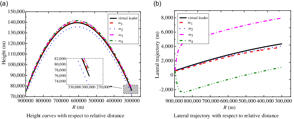
Figure 3. Height and lateral trajectory of flight vehicle.

Figure 4. Configuration parameter curves with respect to time.
The sliding mode curves of three-channels with respect to the flight time for each sub-vehicle are shown in Fig. 5. From Fig. 5(a)–(d), it can be seen that the sliding mode surfaces (see Equation (9)) of three-channels for each sub-vehicle both reach a small neighbor of zero with small oscillation in a finite time, and the convergence time is about
 $118.75{\rm{s}}$
.
$118.75{\rm{s}}$
.
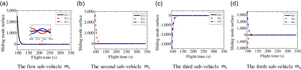
Figure 5. Sliding mode curves of three-channels with respect to time.
To better illustrate the effectiveness of proposed control law, the acceleration commands in the LOS coordinate system can be transferred into the inertial coordinate system, just as shown in Fig. 6. From Fig. 6(a)–(d), it can be seen that the acceleration commands of three-channels firstly occur a sharply jump, and then keep a small amplitude of periodic oscillation patter relative to zero which aims to counteract the effects of the external disturbance and gravitational acceleration of projectile body.

Figure 6. Acceleration command curves of three-channels with respect to time.
It can be observed from Fig. 3, 4, 5 and 6 that the control law shown in Equation (12) can guarantee the rapid generation of the expected formation configuration and ensure that all sub-vehicles simultaneously fly to the preset terminal position, which lays the foundation for the realisation of high precision collaborative detection of the target.
5.2 Simulation results of Case 2
In this section, the initial parameters of each sub-vehicle are listed in Table 2. Considering the dynamic lag time constant of the autopilot
 $\tau =0.5$
for Equation (20), and the control parameter
$\tau =0.5$
for Equation (20), and the control parameter
 ${k_0}=0.03$
, while the other control parameters are the same as in Case 1.
${k_0}=0.03$
, while the other control parameters are the same as in Case 1.
In this case, the trajectory curves of the virtual leader and each sub-vehicle are given in Fig. 7. From Fig. 7(a), the changing trend of the height curves for each sub-vehicle is consistent with the Case 1; however, for the lateral trajectory curves shown in Fig. 7(b), it can be obviously seen that the convergence time is longer compared with the Case 1.

Figure 7. Height and lateral trajectory of flight vehicle.
In this case, the configuration parameters changing curves with respect to the flight time are shown in Fig. 8. From Fig. 8(a)–(c), it can be seen that four sub-vehicles both reach the expected positions, and the convergence time of the formation configuration is about
 $255{\rm{s}}$
.
$255{\rm{s}}$
.
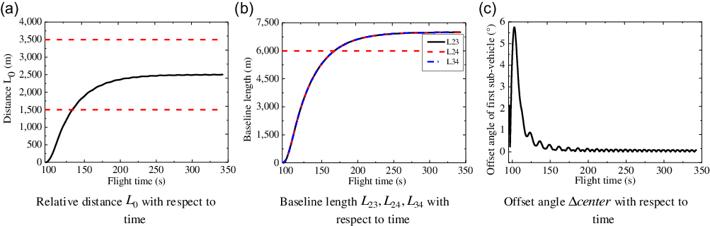
Figure 8. Configuration parameter curves with respect to time.
Taking the
 ${3^{th}}$
sub-vehicle as an example, the sliding mode curves of three-channels with respect to the flight time are shown in Fig. 9(a) and (b), where the sliding mode surfaces
${3^{th}}$
sub-vehicle as an example, the sliding mode curves of three-channels with respect to the flight time are shown in Fig. 9(a) and (b), where the sliding mode surfaces
 ${s_{\rm{1}}}$
and
${s_{\rm{1}}}$
and
 ${s_{\rm{2}}}$
(see Equations (22) and (25)) of the
${s_{\rm{2}}}$
(see Equations (22) and (25)) of the
 ${3^{th}}$
sub-vehicle both converge to near zero with small oscillation induced by the external disturbances. Moreover, the acceleration curves of three-channels for the
${3^{th}}$
sub-vehicle both converge to near zero with small oscillation induced by the external disturbances. Moreover, the acceleration curves of three-channels for the
 ${3^{th}}$
sub-vehicle are shown in Fig. 9(c), where the axial acceleration and lateral acceleration reach around zero while the normal acceleration finally converges to near the gravitational acceleration of projectile body.
${3^{th}}$
sub-vehicle are shown in Fig. 9(c), where the axial acceleration and lateral acceleration reach around zero while the normal acceleration finally converges to near the gravitational acceleration of projectile body.
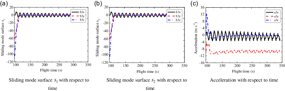
Figure 9. Sliding mode surfaces and accelerations of the third sub-vehicle.
5.3 Simulation results of Case 3
In this section, choose the observer gains in Equation (48) as follows:
 ${\lambda _0}=2,{\lambda _1}=3,{\lambda _2}=5,\delta =30$
; The control parameters in Equation (47) can be designed as follows:
${\lambda _0}=2,{\lambda _1}=3,{\lambda _2}=5,\delta =30$
; The control parameters in Equation (47) can be designed as follows:
 ${k_0}=0.03,\break {t_r}=341.5{\rm{s,}}\ n=2,\eta =5$
, and the dynamic lag time constant of the autopilot is consistent with Case 2. In this case, the configuration parameters changing curves with respect to the flight time under the control law (44) are shown in Fig. 10. From Fig. 10, it can be seen that the formation configuration of the system converges at the desired time
${k_0}=0.03,\break {t_r}=341.5{\rm{s,}}\ n=2,\eta =5$
, and the dynamic lag time constant of the autopilot is consistent with Case 2. In this case, the configuration parameters changing curves with respect to the flight time under the control law (44) are shown in Fig. 10. From Fig. 10, it can be seen that the formation configuration of the system converges at the desired time
 ${t_r}$
, and the control law proposed in the Section 4.3 has high control precision.
${t_r}$
, and the control law proposed in the Section 4.3 has high control precision.
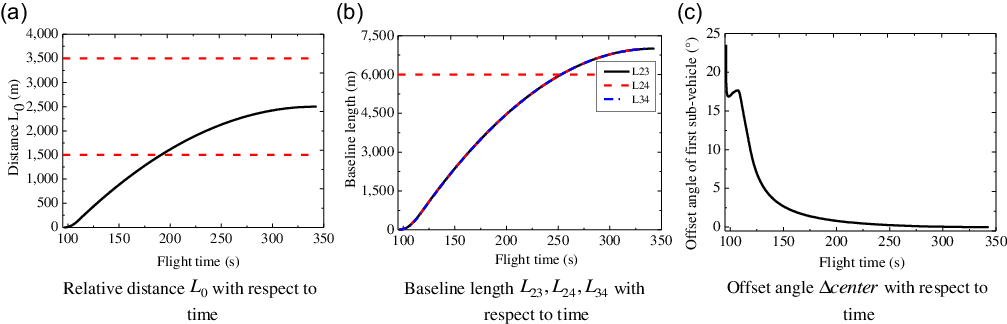
Figure 10. Configuration parameter curves with respect to time.
To compare with Case 2, for the
 ${3^{th}}$
sub-vehicle, the sliding mode curves of three-channels with respect to the flight time are shown in Fig. 11(a) and (b), where the small-amplitude chattering is completely eliminated. The acceleration curves of three-channels for the
${3^{th}}$
sub-vehicle, the sliding mode curves of three-channels with respect to the flight time are shown in Fig. 11(a) and (b), where the small-amplitude chattering is completely eliminated. The acceleration curves of three-channels for the
 ${3^{th}}$
sub-vehicle are shown in Fig. 11(c), where the acceleration responses are smaller than those shown in Fig. 9(c) and without chattering.
${3^{th}}$
sub-vehicle are shown in Fig. 11(c), where the acceleration responses are smaller than those shown in Fig. 9(c) and without chattering.

Figure 11. Sliding mode surfaces and accelerations of the third sub-vehicle.

Figure 12. Gaussian white noise and estimation value.
To further verify the effectiveness of proposed control law, next considering the Gaussian white noise disturbance shown in Fig. 12. For the sliding mode disturbance observer shown in Equation (48), the observer gains are still unchanged. The estimation of the noise is also given after passing through a first-order low pass filter, as shown in Fig. 12.

Figure. 13. Sliding mode surfaces and accelerations of the first sub-vehicle.

Figure 14. Sliding mode surfaces and accelerations of the second sub-vehicle.

Figure 15. Sliding mode surfaces and accelerations of the third sub-vehicle.
Under the effect of Gaussian noise, the control parameters in Equation (47) remain the same. For the formation system, the sliding mode curves and acceleration curves of three-channels with respect to the flight time are shown in Fig. 13, 14, 15 and 16. It is obvious that for the Gaussian white noise disturbance, the sliding mode surfaces
 ${s_{\rm{1}}}$
(see Equation (22)) still converges to zero at the expected time, which means that the four sub-vehicles can form the expected formation configuration. Besides, for the sliding mode surfaces
${s_{\rm{1}}}$
(see Equation (22)) still converges to zero at the expected time, which means that the four sub-vehicles can form the expected formation configuration. Besides, for the sliding mode surfaces
 ${s_2}$
(see Equation (40)) and accelerations, they all converge in a finite time and the chattering is effectively suppressed during the flight.
${s_2}$
(see Equation (40)) and accelerations, they all converge in a finite time and the chattering is effectively suppressed during the flight.

Figure 16. Sliding mode surfaces and accelerations of the fourth sub-vehicle.
6.0 CONCLUSION
In this paper, the cooperative control problem of space formation configuration for four reentry vehicles equipped with radar detector is researched during the mid-guidance phase. The expected position vector of each sub-vehicle is designed firstly according to the configuration constraints proposed based on a specific flight scenario. The adaptive second-order sliding mode controller is designed with considering the external disturbance and system noise, and the first-order dynamic characteristic of the autopilot. The conclusions of the investigations in this paper are listed as follows.
-
(1) The formation controlling errors can simultaneously converge to the neighbor of zero in a finite time, which means that the configuration constraints can be met effectively under the effect of the external disturbance and system noise.
-
(2) The maximum required acceleration for each sub-vehicle is reduced, and the chattering phenomenon of the sliding surfaces and the acceleration responses can be effectively suppressed, which is of great significance in engineering.
DATA AVAILABILITY
The data used to support the findings of this study are available from the corresponding author upon request.
CONFLICTS OF INTEREST
The authors declare that there is no conflict of interests regarding the publication of this paper.