2.1. Governing equations

Compressible RT turbulence is started from the hydrostatic equilibrium of a layer of heavy fluid on top of a layer of lighter fluid, for which direct numerical simulation has been carried out by solving the mass, momentum and energy equations. We employ the initial pressure ($p_I$) and density ($\rho _I$) at the heavy fluid–light fluid interface as characteristic scales, where $\rho _I=(\rho _1+\rho _2)/2$ with $\rho _1$ and $\rho _2$ being the densities at the upper and lower surfaces of the initial interface. Then a characteristic temperature is represented as $T_I=p_I/(R\rho _I)$, with $R$ being the perfect gas constant, and a characteristic velocity as $U_I=\sqrt {p_{I}/\rho _{I}}$. The vertical length ($L_z$) of the flow domain is chosen as the characteristic length. Accordingly, the non-dimensionalized governing equations are given as

(2.1)\begin{gather} \frac{\partial\rho}{\partial t}+\frac{\partial(\rho u_{i})}{\partial x_{i}} =0, \end{gather}

(2.2)\begin{gather}\frac{\partial(\rho u_{i})}{\partial t}+\frac{\partial(\rho u_{i}u_{j})}{\partial x_{j}} =-\frac{\partial p}{\partial x_{i}}+\frac{1}{Re}\frac{\partial\tau_{ij}}{\partial x_{j}} -\frac{1}{Fr}\rho\delta_{i3}, \end{gather}

(2.3)\begin{gather}\frac{\partial(\rho e)}{\partial t}+\frac{\partial(\rho e+p)u_{i}}{\partial x_{i}} =\frac{1}{Re}\frac{\partial (u_{i}\tau_{ij})}{\partial x_{j}} +\frac{1}{RePr}\frac{\partial}{\partial x_{i}}\left(\frac{\partial T}{\partial x_{i}}\right) -\frac{1}{Fr}\rho u_{3}, \end{gather}

where $\rho$ is the fluid density, $u_{i}$ ($i=1$, 2 and 3) is the velocity component in the $x_i$ direction, or $(u_1, u_2, u_3)=(u, v, w)$ in $(x_1, x_2, x_3)=(x, y, z)$, $p$ is the pressure, $T$ is the temperature and $e$ denotes the specific total energy obtained as $e=T/(\gamma -1)+u_{i}u_{i}/2$ with the ratio of specific heat $\gamma =1.4$. The viscous stress $\tau _{ij}$ is represented as

(2.4)\begin{equation} \tau_{ij}=\mu\left(\frac{\partial u_{i}}{\partial x_{j}}+\frac{\partial u_{j}}{\partial x_{i}}\right) -\frac{2}{3}\mu\theta\delta_{ij}, \end{equation}

where $\theta =\partial u_{k}/\partial x_{k}$ is the dilatation related to the compression/expansion motions of fluid parcels and $\mu =T^{3/2}(1+c)/(T+c)$ is the viscosity computed by the Sutherland law with $c=110/T_{r}$ and the reference temperature $T_{r}$. The above governing equations are closed with the equation of state of an ideal gas, i.e. $p=\rho T$.

The non-dimensional parameters in the governing equations (2.1)–(2.3) are the Reynolds, Froude and Prandtl numbers defined as

(2.5a–c)\begin{equation} Re=\frac{\rho_{I}U_{I}L_{z}}{\mu_{I}}, \quad Fr=\frac{U_{I}^{2}}{L_{z} g} \quad \textrm{and} \quad Pr=C_{p}\frac{\mu_{I}}{\kappa},\end{equation}

respectively, where $g$ is the gravitational acceleration imposed opposite to the vertical direction, $C_{p}$ the specific heat at constant pressure and $\kappa$ the thermal conductivity.

2.2. Numerical simulations

Both the heavy and lighter layers are initialized as the buoyancy-stable configuration, which is indicated to have considerable flow compressibility effects (Mellado et al. Reference Mellado, Sarkar and Zhou2005). Specifically, the heavy fluid is set at uniform temperature $T_{up}=1/(1-At)$ above the interface ($z>0$) and the lighter fluid at $T_{low}=1/(1+At)$ below the interface ($z<0$), where the Atwood number $At$ is defined as

(2.6)\begin{equation} At=\frac{\rho_1-\rho_2}{\rho_1+\rho_2}. \end{equation}

Correspondingly, the hydrostatic equilibrium state is obtained from the governing equations (2.1)–(2.3) by setting $u_{i}$ to be zero for a stationary solution. This solution is a potentially unstable stack of two stable exponentially stratified profiles:

(2.7)\begin{equation} \rho=(1+At)\exp\left(-\frac{1+At}{Fr}z\right)H^{+}(z)+ (1-At)\exp\left(-\frac{1-At}{Fr}z\right)H^{-}(z), \end{equation}

where $H(z)$ is the Heaviside step function, and its upper symbols $+$ and $-$ represent the upper and lower side of the interface, respectively. The interface at $z=0$ is perturbed by a superposition of cosine waves along the horizontal directions, i.e. $A_m \cos (2{\rm \pi} k_{x}x/L_{x}+\phi _{k})\cos (2{\rm \pi} k_{y}y/L_{y}+\psi _{k})$, where the perturbation wavenumbers $k_{x}$ and $k_{y}$ in the $x$ and $y$ directions are set in a range of $30\leq k_{x}$ (or $k_{y}$) $\leq 60$ with the amplitude $A_m=10^{-4}$ and random phases $\phi _{k}$ and $\psi _{k}$ (Clark Reference Clark2003; Boffetta et al. Reference Boffetta, Mazzino, Musacchio and Vozella2009; Qiu, Liu & Zhou Reference Qiu, Liu and Zhou2014).

In order to generate strong turbulence (Dimotakis Reference Dimotakis2000; Cabot & Cook Reference Cabot and Cook2006; Cabot & Zhou Reference Cabot and Zhou2013), we use a high Atwood number of $At=0.6$ (Bian et al. Reference Bian, Aluie, Zhao, Zhang and Livescu2020) with $Re=10^{5}$. The Froude number is fixed at $Fr=1$. The RT flow is considered as homogeneous in the horizontal directions and thus periodic boundary conditions are used. There is no mass and heat flux through the top and bottom boundaries (Gauthier Reference Gauthier2017). The computational domain is set as $L_{x}\times L_{y} \times L_{z}=0.5\times 0.5\times 1$ in the $x$, $y$ and $z$ (vertical) directions, respectively. It is resolved by uniform grids of size $650\times 650\times 1300$. Similar to the numerical schemes used by Zhou, Zhang & Tian (Reference Zhou, Zhang and Tian2018) and Li et al. (Reference Li, He, Zhang and Tian2019), the seventh-order finite difference WENO scheme is implemented to discretize the convective terms (Jiang & Shu Reference Jiang and Shu1996) and the eighth-order central difference scheme to discretize the viscous terms. The time derivative is approximated by the standard third-order Runge–Kutta method.

2.3. Grid resolution tests and flow features

To ensure that the grid resolution used is sufficient for the present direct numerical simulation, we examine the Kolmogorov length scale in the turbulent mixing zone, which is calculated by

(2.8)\begin{equation} \eta=\frac{1}{\sqrt{Re}}\frac{1}{\sqrt{\langle\rho\rangle}} \left(\frac{\langle{\mu}\rangle^{3}}{\langle\varepsilon\rangle}\right)^{1/4},\end{equation}

where $\varepsilon$ is the viscous dissipation rate and $\langle\, f \rangle =(L_xL_yh)^{-1}\int _{h_S}^{h_B}\iint f \,\mathrm {d} x\,\mathrm {d} y \,\mathrm {d} z$ denotes the volume average in the mixing region. Here, $h$ means the entrainment width of mixing region, where the entrained fluids are perfectly homogenized in the horizontal plane (Cabot & Cook Reference Cabot and Cook2006), and is the sum of the mean thicknesses of bubbles and spikes (Gauthier Reference Gauthier2017), i.e. $h_{B}$ and $h_{S}$:

(2.9a,b)\begin{equation} h_{S}=\int_{-{L_{z}}/{2}}^{0} M(\bar{T})\,\mathrm{d} z \quad \textrm{and} \quad h_{B}=\int^{{L_{z}}/{2}}_{0} M(\bar{T})\,\mathrm{d} z. \end{equation}

Here, a mixing function $M(T)=4(T-T_{up})(T_{low}-T)/(T_{low}-T_{up})^{2}$ is employed with $0\leq M\leq 1$ (Dalziel, Linden & Youngs Reference Dalziel, Linden and Youngs1999; Vladimirova & Chertkov Reference Vladimirova and Chertkov2009) and the overbar denotes the spatial average in the horizontal plane.

To ensure the reliable prediction of statistics by means of direct numerical simulation, as indicated by Yeung & Pope (Reference Yeung and Pope1989), a resolution criterion of $k_{max}\eta \geq 1$ is adequate for low-order velocity statistics, while a criterion of $k_{max}\eta \geq 1.5$ is required for higher-order statistics (such as dissipation rate statistics), where $k_{max}$ stands for the maximum wavenumber resolved. As shown in figure 1(a), the normalized Kolmogorov length scale $k_{max}\eta$ decreases gradually for $t/\tau <1.5$ and approaches a plateau value $\sim$3 when $t/\tau >2$, where $\tau =(L_{z} Fr/At)^{1/2}$ is the characteristic time of the RT flow (Kord & Capecelatro Reference Kord and Capecelatro2019). This behaviour is well captured for the evolution of RTI from the early stage to turbulent mixing. Furthermore, it is identified that $\eta /\varDelta \simeq 1.0$ at $t/\tau =3.0$, where $\varDelta$ is the grid width used in this study. Thus the present grid resolution can reliably predict the compressible RT flow and is enough to properly capture the smallest scales of the flow.

Figure 1. Evolution of the mean normalized Kolmogorov length scale (a) and outer scale Reynolds number (b).

Moreover, the evolution of RT flow can be measured in terms of the so-called outer scale Reynolds number defined as $Re_{H}=\rho _{I}H\dot {H}/\mu _{I}$ (Cook & Zhou Reference Cook and Zhou2002; Cabot & Cook Reference Cabot and Cook2006), where $H$ is the visual width of mixing region defined as the mean vertical range with the mixing function $M(\bar {T})>0.01$. Here $H=2.1h$ has been used to ensure $M(\bar {T})>0.01$ in the mixing region. Usually a critical $Re_{H}$ value ${\sim }10^{4}$ is required for a mixing transition to fully developed turbulence (Dimotakis Reference Dimotakis2000). It is seen from figure 1(b) that $Re_{H}$ has a significant increase to the order of ${\sim }10^{4}$ at $t/\tau \approx 2$, and then up to $2.6\times 10^{4}$ at $t/\tau =3.0$. It is identified that the Reynolds number grows with a $t^{3}$ scaling for $t/\tau >2$ approximately, which means a fully developed state is achieved in the mixing region of the RT flow (Cook & Zhou Reference Cook and Zhou2002).

Further, the kinetic energy spectra are employed to determine that the grid resolution used is fine enough. Figure 2(a) shows the kinetic energy spectra $E(k)$ calculated in the horizontal plane at $z=0$ at $t/\tau =1.0$, $2.0$ and $3.0$. Two typical features are demonstrated obviously in the spectra $E(k)$ versus time: an increase of peak value up to several orders shifting towards low wavenumbers and an occurrence of an inertial range as evidenced by the well-fitted power law. The former feature indicates an increasing dominance of larger-scale structures that are formed due to the merging of bubbles and spikes. This is facilitated by the continuous energy injection as the buoyancy converts energy from potential to kinetic energy. The latter implies that a fully developed state of turbulent mixing is realized at approximately $t/\tau =2.0$. Note that the spectra obtained are consistent with a power law of $-7/4$ for the inertial range predicted by Zhou (Reference Zhou2001), different from the classical Kolmogorov law, i.e. $-5/3$. This feature is reasonably related to the external time scale introduced by the buoyancy (Cook & Zhou Reference Cook and Zhou2002). Further, figure 2(b) shows the velocity spectra $E_{u}(k)$, $E_{v}(k)$ and $E_{w}(k)$ at $t/\tau =3.0$. The velocity spectra exhibit stronger anisotropy at large scales than at small scales. In particular, $E_{w}(k)$ is higher by about one order of magnitude than $E_{u}(k)$ and $E_{v}(k)$ at large scales.

Figure 2. Kinetic energy spectra $E(k)$ (a) at instants $t/\tau =1.0$, $2.0$ and $3.0$ and velocity spectra (b) at $t/\tau =3.0$ in the horizontal plane at $z=0$. Here, the horizontal wavenumber $k=\sqrt {k_x^{2}+k_y^{2}}$.

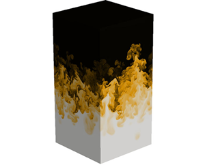
The flow structures are well captured for RT turbulence under the present grid resolution. Figure 3 typically shows a snapshot of the instantaneous temperature field at $t/\tau =3.0$. It exhibits fine-scale structures and large patches of mixed fluids. Specifically, large-scale structures are well identified in the turbulent mixing zone, which arise as the merging of bubbles and spikes. Small-scale structures are also fully resolved along the evolutional interface between the hot (ascending) and cold (descending) fluids. This visualization indicates clearly the non-stationary and non-isotropic feature of compressible RT turbulence (Boffetta et al. Reference Boffetta, Mazzino, Musacchio and Vozella2009).

Figure 3. Snapshot of instantaneous temperature field for compressible RT turbulence at $t/\tau =3.0$. Here, white and black colour regions represent the hot and cold fluids, respectively.

In addition, we have carefully examined the physical model and numerical approach used in this study and have verified that the calculated results are reliable in our previous work on compressible turbulent boundary layer (Wang & Lu Reference Wang and Lu2012; Chu & Lu Reference Chu and Lu2013) and on compressible turbulent mixing layer (Yu & Lu Reference Yu and Lu2019, Reference Yu and Lu2020).

3.1. Generation of kinetic energy

Energy conversion from potential to kinetic energy is first investigated in compressible RT flows by means of the kinetic energy budget. From the momentum equation (2.2) the transport equation of kinetic energy is derived as

(3.1)\begin{equation} \frac{\partial}{\partial t}\left(\frac{1}{2}\rho u_{i}u_{i}\right)+ \frac{\partial}{\partial x_{j}}\left(\frac{1}{2}\rho u_{i}u_{i}u_{j}+pu_{j}- \frac{1}{Re}u_{i}\tau_{ij}\right) =p\theta-\frac{1}{Re}\tau_{ij}\frac{\partial u_{i}}{\partial x_{j}} -\frac{1}{Fr}\rho u_{3}. \end{equation}

By integrating equation (3.1) over the flow domain, we have the global kinetic energy budget

(3.2)\begin{equation} -\frac{\mathrm{d} P}{\mathrm{d} t}+W=\frac{\mathrm{d} K}{\mathrm{d} t}+\varepsilon, \end{equation}

where $P=({1}/{Fr})\int _{V}\rho z\,\mathrm {d} V$ is the potential energy, $K=\int _{V}\frac {1}{2}\rho u_{i}u_{i}\,\mathrm {d} V$ is the kinetic energy, $\varepsilon =({1}/{Re})\int _{V}\tau _{ij}({\partial u_{i}}/{\partial x_{j}})\,\mathrm {d} V$ is the energy dissipation rate and $W=\int _{V}p\theta \,\mathrm {d} V=\int _{V}p({\partial u_{k}}/{\partial x_{k}})\,\mathrm {d} V$ is the pressure-dilatation power term. Note that the pressure-dilatation power term is related to the power of pressure work due to the compressing process in compressible RT flows, which plays an important role in the local conversion between kinetic energy and internal energy (Wang et al. Reference Wang, Wan, Chen and Chen2018). A positive $W$ means that the dilatation effect contributes to the generation of kinetic energy, and vice versa. Moreover, the other terms integrated in (3.1) vanish because the periodic and flux-free conditions are applied in the horizontal and vertical boundaries, respectively.

Based on (3.2), it is identified that there exist two mechanisms for the generation of kinetic energy, namely the conversion of potential energy to kinetic energy and the pressure work related to the compressibility of fluid elements. Thus, the two mechanisms are first investigated based on the budget terms of (3.2). As shown in figure 4, ${\mathrm {d} K}/{\mathrm {d} t}$ remains positive during flow evolution, which means a continuous increase of the kinetic energy. This behaviour is associated with two factors as indicated in (3.2). The term ${\mathrm {d} P}/{\mathrm {d} t}$ is a negative distribution, which means the persisting conversion of potential energy into kinetic energy. In reality, the conversion acts as a major mechanism for the generation of kinetic energy as evidently shown for $t/\tau >1$. Rather than trivial as in incompressible RT flows (Cabot & Cook Reference Cabot and Cook2006; Zhou Reference Zhou2013), the pressure-dilatation power $W$ is comparable to ${\mathrm {d} K}/{\mathrm {d} t}$, especially at $t/\tau \approx 1.2$ and $2.8$ where two peaks occur obviously. The evolution of $W$ reveals that the dilatation effects serve as an important source to generate kinetic energy in the development of RT turbulence. Moreover, $\varepsilon$ increases with flow evolution to account for the kinetic energy dissipation.

Figure 4. Evolution of the budget terms of kinetic energy in (3.2).

The overall energy balance can be quantified by taking a temporal integration of (3.2) from $0$ to $t$, which gives

(3.3)\begin{equation} -\delta P(t)+\delta W(t)=\delta K(t)+\varPsi(t), \end{equation}

where $-\delta P(t)$ is the total potential energy, $\delta W(t)$ is the total pressure-dilatation work related to the overall dilatation effect, $\delta K(t)$ is the total kinetic energy increase of the RT system considered and $\varPsi (t)$ is the total energy dissipation. It is identified from (3.3) that the total input energy for the RT system is responsible for the total production, i.e. $-\delta P+\delta W$. Therefore, the overall production efficiency of kinetic energy can be evaluated by the ratio $\delta K / (-\delta P+\delta W)$ and the overall dilatation effect on the generation of kinetic energy by the ratio $\delta W/(-\delta P+\delta W)$.

Figure 5 shows the two ratios during the evolution of compressible RT flow. The overall production efficiency $\delta K / (-\delta P+\delta W)$ increases gradually from $20\,\%$ in the early stage and reaches a level of over $50\,\%$. Then it decreases slightly to around $45\,\%$ in the later stage. When the ratio $\delta W/(-\delta P+\delta W)$ is around 1, it means that the dilatation effect is almost fully responsible for the generation of kinetic energy. This behaviour is related to the non-uniform initial temperature induced by a non-zero time derivative in energy equation (2.3), i.e. $\partial _{t}(\rho e)=({1}/{RePr}) \partial _{j}(\partial _{j} T)$. For the compressible RT flow considered here, the dilatational velocity can be demonstrated by the contour patterns of dilatation as shown in figure 6. It is seen that the dilatation patterns of $\theta >0$ appear in the regions with relatively higher pressure and vice versa, accounting for the prevailing contribution of $\delta W(t)$ to the generation of kinetic energy. The overall dilatation effect remains prevalent over the conversion of potential energy for $t/\tau <1.5$ approximately as the ratio $\delta W/(-\delta P+\delta W) > 0.5$. Then this situation changes for $t/\tau >1.5$ as $\delta W/(-\delta P+\delta W)< 0.5$. In turbulent mixing, this ratio reaches $0.1$–$0.2$, indicating that the conversion of potential energy offers the main contribution to the kinetic energy rather than the pressure-dilatation work.

Figure 5. Ratios of the total kinetic energy change to total production and of the pressure-dilatation work to total production.

Figure 6. Contour plots of dilatation (coloured pattern) and pressure (coloured line) near the interface at $t/\tau =0.16$ in (a) the $y$–$z$ plane at $x=0.25$ and (b) the $x$–$z$ plane at $y=0.25$.

In order to clarify the effect of kinetic energy generation mechanisms on compressible RT turbulence, we investigate the scaling exponents of longitudinal velocity structures by means of the approaches used for two-dimensional incompressible RT turbulence (e.g. Celani, Mazzino & Vozella Reference Celani, Mazzino and Vozella2006) and for three-dimensional incompressible RT turbulence (e.g. Matsumoto Reference Matsumoto2009). Figure 7(a) shows the temporal scaling of the velocity structure functions at spatial scale $x/L_x=0.1$, which is chosen based on the fact that this spatial scale lies in the inertial range from the kinetic energy spectra in figure 2(a). It is identified that there exist two scaling exponents for two typical stages of developing state for $t/\tau < 1.5$ approximately and fully developed state for $t/\tau > 2.0$ of turbulent mixing. According to the results shown in figure 5, the reason is possibly associated with different mechanisms of kinetic energy generation in the two stages. The pressure-dilatation work dominates the generation of kinetic energy for $t/\tau < 1.5$, while the potential energy conversion provides the main contribution for $t/\tau > 2.0$. Hence, the scaling exponents in the fully developed state ($t/\tau > 2.0$) in figure 7(a) agree quite well with the phenomenological predictions (Chertkov Reference Chertkov2003), i.e. $\delta _ru\sim (Atg)^{2/3}r^{1/3}t^{1/3}$, for incompressible RT turbulence at the fully developed stage in which the potential energy conversion dominates the generation of kinetic energy.

Figure 7. Longitudinal velocity structures $\langle (\delta _xu_1)^{p}\rangle$ along the $x$ direction, where $u_1$ is the $x$ component of the velocity, as functions of (a) time $t/\tau$ at spatial scale $x/L_x=0.1$ and (b) distance $x/L_x$ at time $t/\tau =3.0$. Solid lines represent the phenomenological predictions by Chertkov (Reference Chertkov2003). Dashed lines represent the fitted curve slopes.

Figure 7(b) also shows the spatial scaling of the velocity structure functions at time $t/\tau =3.0$ when a fully developed state is achieved in the mixing region of RT flow. It is seen that the scaling exponents of the second-order velocity structure functions are approximately consistent with the phenomenological predictions (Chertkov Reference Chertkov2003). However, the scaling exponents of the higher-order velocity structure functions no longer agree with the phenomenological predictions (Chertkov Reference Chertkov2003). Such obvious deviations were also reported by Matsumoto (Reference Matsumoto2009) for three-dimensional incompressible turbulence. The possible reason for these obvious deviations may be related to the anisotropic behaviour in RT turbulence and the narrow inertial range at relatively low Reynolds number.

3.2. Transfer of kinetic energy

The scale-to-scale transfer of kinetic energy is investigated for compressible RT turbulence. The relevant problem has never been discussed before. Here we apply a recently developed filtering approach (Aluie Reference Aluie2011, Reference Aluie2013; Wang et al. Reference Wang, Yang, Shi, Xiao, He and Chen2013) to analyse the kinetic energy transfer. A filter operator is represented as

(3.4)\begin{equation} \bar{f}_{r}(\boldsymbol{x})=\int G_{r}(\boldsymbol{x}')f(\boldsymbol{x}+\boldsymbol{x}')\,\mathrm{d} \boldsymbol{x}', \end{equation}

where $G_{r}$ is a Gaussian filter and the subscript $r$ denotes a function $f$ containing the information only at length scales larger than $r$. For the present compressible RT turbulence, the Favre filter is also used and defined as $\tilde {f}=\overline{\rho f}/\bar {\rho }$. Then a large-scale kinetic energy equation (Aluie Reference Aluie2011, Reference Aluie2013; Wang et al. Reference Wang, Yang, Shi, Xiao, He and Chen2013) can be given as

(3.5)\begin{equation} \frac{\partial}{\partial t}\left(\frac{\bar{\rho}_{r}|\tilde{\boldsymbol{u}}_{r}|^{2}}{2}\right) +\boldsymbol{\nabla}\boldsymbol{\cdot}\boldsymbol{J}_{r}=-\varPi_{r}-\varLambda_{r}+\varPhi_{r}-\varepsilon_{r}+I_{r}, \end{equation}

where $\frac {1}{2}\bar {\rho }_{r}|\tilde {\boldsymbol {u}}_{r}|^{2}$ is the large-scale kinetic energy and the other terms are defined as

(3.6a)\begin{gather} \left(\boldsymbol{J}_{r}\right)_{j} = \bar{\rho}\frac{|\tilde{\boldsymbol{u}}_{r}|^{2}}{2}\tilde{u}_{j} +\overline{pu}_{j} +\tilde{u}_{i}\bar{\rho}\left(\widetilde{u_{i}u_{j}}-\tilde{u}_{i}\tilde{u}_{j}\right) -\frac{1}{Re}\tilde{u}_{i}\bar{\tau}_{ij}, \end{gather}

(3.6b)\begin{gather}\varPi_{r} = -\bar{\rho}\left(\widetilde{u_{i}u_{j}}-\tilde{u}_{i}\tilde{u}_{j}\right) \frac{\partial\tilde{u}_{i}}{\partial x_{j}}, \end{gather}

(3.6c)\begin{gather}\varLambda_{r} = \frac{1}{\bar{\rho}}\frac{\partial\bar{p}}{\partial x_{j}}\left(\overline{\rho u_{j}}-\bar{\rho}\,\bar{u}_{j}\right), \end{gather}

(3.6d)\begin{gather}\varPhi_{r} = \bar{p}\,\frac{\partial\bar{u}_{i}}{\partial x_{i}}, \end{gather}

(3.6e)\begin{gather}\varepsilon_{r} = \frac{1}{Re}\bar{\tau}_{ij}\frac{\partial\tilde{u}_{i}}{\partial x_{j}}, \end{gather}

(3.6f)\begin{gather}I_{r} = -\frac{1}{Fr}\bar{\rho}\tilde{u}_{3}. \end{gather}

Here, $\boldsymbol {J}_{r}$ is the spatial transport of the large-scale kinetic energy; $\varPi _{r}$ is the deformation work done by large-scale strain ${\partial \tilde {u}_{i}}/{\partial x_{j}}$ against the subgrid stress $\bar {\rho }(\widetilde {u_{i}u_{j}} -\tilde {u}_{i}\tilde {u}_{j})$, which represents the kinetic energy transfer from the filtered scale to smaller scale; $\varLambda _{r}$ is the baropycnal work done by the large-scale pressure gradient $({1}/{\bar {\rho }})({\partial \bar {p}}/{\partial x_{j}})$ against the subscale mass flux $\overline {\rho u_{j}}-\bar {\rho }\,\bar {u}_{j}$ (Aluie Reference Aluie2011, Reference Aluie2013), which also means the kinetic energy transfer to scales smaller than $r$; $\varPhi _{r}$ is the large-scale pressure dilatation related to the flow compressibility; $\varepsilon _{r}$ is the large-scale viscous dissipation term; and $I_{r}$ is the energy injected by gravity.

Figure 8 shows the terms on the right-hand side of (3.5) averaged in the mixing region versus the normalized filter scale $r/\eta$ at several instants $t/\tau =1.0$, $2.0$ and $3.0$. It is seen that the kinetic energy is generated by the pressure dilatation $\varPhi _{r}$ and the injection of gravity $I_{r}$ at all scales. The pressure dilatation is larger than the injection of gravity at $t/\tau =1.0$, then becomes less than the injection of gravity at $t/\tau =2.0$ and $3.0$, which differs from Boussinesq RT turbulence where kinetic energy is only generated by gravity at all scales (Chertkov Reference Chertkov2003; Zhou et al. Reference Zhou, Huang, Lu, Liu and Ni2016). This behaviour indicates that the compressibility plays as an important role in the generation of kinetic energy at all scales. The kinetic energy is dissipated by the viscous effect and the viscous dissipation becomes stronger at smaller scales. Furthermore, the characteristics of the deformation work and the baropycnal work are worthy of concern. The deformation work is negative in the large filter scales at $t/\tau =1.0$, then becomes positive at $t/\tau =2.0$ and $3.0$, since the formation of large-scale structures caused by the merger of bubbles and spikes allows the kinetic energy transfer from large to small scales. Then the peak of deformation work is gradually formed at the filter scale $r/\eta \approx 50$ with the flow evolution. The baropycnal work is always positive in all scales, indicating that the kinetic energy is transferred from large to small scales under its action and the kinetic energy transfer becomes stronger with an increase of the scale. Based on the investigation of Lees & Aluie (Reference Lees and Aluie2019) in compressible isotropic homogeneous turbulence (IHT), the baropycnal work occurs only in variable density flows. This is well consistent with the physical mechanisms of compressible IHT that the baropycnal work arises in RT turbulence which is a canonical variable density flow. However, different from compressible RT turbulence, the baropycnal work in compressible IHT is negative (Wang et al. Reference Wang, Yang, Shi, Xiao, He and Chen2013; Lees & Aluie Reference Lees and Aluie2019) and the total amount of energy transfer across scales is effectively reduced. Moreover, the pressure and density gradients in compressible IHT have the same direction to align with the contracting strain eigenvector across a shock, leading to negative baropycnal work (Lees & Aluie Reference Lees and Aluie2019). In the mixing region of RT turbulence, the pressure and density gradients have the opposite direction, resulting in positive baropycnal work. By comparing the deformation work with the baropycnal work, it is found that the deformation work is greater than the baropycnal work in small filter scales, while it becomes less than the baropycnal work in large filter scales.

Figure 8. The average terms of the large-scale kinetic energy equation versus the normalized filter scale $r/\eta$ at different instants: (a) $t/\tau =1.0$, (b) $t/\tau =2.0$ and (c) $t/\tau =3.0$.

Further we investigate the deformation work and the baropycnal work at three filter scales $r/\eta =10$, $50$ and $100$, as shown in figure 9. It is seen that a peak of the baropycnal work occurs and increases with an increase of filter scale. The deformation work is strengthened gradually over time and becomes stabilized approximately for RT turbulence. Meanwhile a negative value in the early stage of flow evolution occurs at $r/\eta =50$ and $100$ because the large-scale structure has not formed yet. The deformation work becomes greater than the baropycnal work at $r/\eta =10$ and $50$ at the late stage. It is also noticed that the baropycnal work is always greater than the deformation work at $r/\eta =100$. The underlying mechanisms can be analysed as follows. Both the deformation work and the baropycnal work reflect that the kinetic energy is transferred from large to small scales. The deformation work plays a major role in scale-to-scale kinetic energy transfer in the small-scale regime, while the baropycnal work plays a major role in scale-to-scale kinetic energy transfer in the large-scale region for RT turbulence.

Figure 9. The average deformation work and baropycnal work versus time at different filter scales: (a) $r/\eta =10$, (b) $r/\eta =50$ and (c) $r/\eta =100$.

As mentioned above, a peak of the baropycnal work occurs. The baropycnal work is done by the large-scale pressure gradient against the subscale mass flux. Therefore, when the entrainment width of the mixing region equals the filter scale, the baropycnal work will achieve the maximum value as the appearance of more subscale mass flux in the mixing region. To verify the above analysis, a characteristic time $t^{*}$ when $h=r$ is defined. Figure 10(a) shows the normalized entrainment width of mixing region $h/\eta$ versus time. Three characteristic times $t_1^{*}=0.55$, $1.01$ and $1.29$ are determined for the filter scales $r/\eta =10$, $50$ and $100$, respectively. Further, the baropycnal work at three filter scales $r/\eta =10$, $50$ and $100$ versus the renormalized time $t/t^{*}$ is shown in figure 10(b). It is seen that the peaks of baropycnal work at different filter scales occur at the corresponding characteristic times approximately.

Figure 10. (a) The normalized entrainment width of mixing region $h/\eta$ versus time. (b) The average baropycnal work versus the renormalized time at three different filter scales.

3.3. Effect of compressibility on baropycnal work

The baropycnal work is the work done by large-scale pressure gradient against the subscale mass flux, which is intrinsically due to the compressibility effect and vanishes in the absence of density variations (Aluie Reference Aluie2013). To reveal the relationship between the baropycnal work and compressibility, we decompose the baropycnal work $\varLambda _{r}$ into a positive component $\varLambda _{r}^{+}$ and a negative component $\varLambda _{r}^{-}$, which are defined as

(3.7a,b)\begin{equation} \varLambda_{r}^{+}=\tfrac{1}{2}(\varLambda_{r}+|\varLambda_{r}|), \quad \varLambda_{r}^{-}=\tfrac{1}{2}(\varLambda_{r}-|\varLambda_{r}|). \end{equation}

Figure 11 shows the positive and negative components of baropycnal work averaged in the mixing region as a function of the normalized filter scale $r/\eta$ at $t/\tau =1.0$, $2.0$ and $3.0$. It is found that the positive component acts a major contribution to the baropycnal work. The behaviour indicates that the kinetic energy transfer caused by the baropycnal work is mainly transferred from large to small scales. As a vertically downward large-scale pressure gradient occurs in the flow field under the action of gravity, the downward movement of the small-scale spike structures makes the baropycnal work positive, and the upward movement of the small-scale bubble structures makes the baropycnal work negative. Since the density of the spike structures is large and the density of the bubble structures is small, the baropycnal work is positive and the kinetic energy is transferred from large to small scales. The larger the filter scale, the greater is the positive component of baropycnal work, because it contains more small-scale bubble and spike structures at the larger filter scales.

Figure 11. The positive and negative components of baropycnal work versus the normalized filter scale $r/\eta$ for different instants: (a) positive components; (b) negative components.

In order to deal with the effect of compressibility on the baropycnal work, we consider the following conditional average of the positive and negative components of baropycnal work, i.e. $\langle \varLambda _{r}^{+}\mid \theta _{r}>0\rangle$, $\langle \varLambda _{r}^{+}\mid \theta _{r}<0\rangle$, $\langle \varLambda _{r}^{-}\mid \theta _{r}>0\rangle$ and $\langle \varLambda _{r}^{-}\mid \theta _{r}<0\rangle$, where $\theta _{r}$ is the filtered velocity divergence. Figure 12 shows the conditional average of the positive and negative components of baropycnal work versus the normalized filter scale $r/\eta$ at $t/\tau =1.0$, $2.0$ and $3.0$. For the conditional average of the positive component, the conditional average for $\theta _{r}>0$ is greater than that for $\theta _{r}<0$. However, for the conditional average of the negative component, the conditional average for $\theta _{r}>0$ is less than that for $\theta _{r}<0$. Therefore, the expansion motion ($\theta _{r}>0$) enhances the positive baropycnal work so that the kinetic energy is transferred from large to small scales, while the compression motion ($\theta _{r}<0$) strengthens the negative baropycnal work so that the kinetic energy is transferred from small to large scales.

Figure 12. Conditional average of the positive and negative components of baropycnal work versus the normalized filter scale $r/\eta$ for different instants.

To further illustrate the relationship between the baropycnal work and compressibility, figure 13 shows the joint probability density function (p.d.f.) of the normalized baropycnal work $\varLambda _{r}/(\varLambda _{r})_{rms}$ and the velocity divergence $\theta _{r}/(\theta _{r})_{rms}$ for the filter scale $r/\eta =50$ at $t/\tau =1.0$, $2.0$ and $3.0$. At $t/\tau =1.0$, the shape of the joint p.d.f. is approximately symmetric with respect to $\theta _{r}/(\theta _{r})_{rms}=0$. At $t/\tau =2.0$ and $3.0$, the shape of the joint p.d.f. is asymmetric with the larger probability in the first and third quadrants. This means that the expansion regions provide a major contribution to the positive component of the baropycnal work and the compression regions to the negative component of the baropycnal work. Because of the compressibility effect, the expansion motion enhances the positive baropycnal work so that the kinetic energy is transferred from large to small scales, and the compression motion strengthens the negative baropycnal work so that the kinetic energy is transferred from small to large scales. Since a vertical downward pressure gradient occurs, the large-density spike structures move downward and the small-density bubble structures move upward, resulting in the baropycnal work being mainly positive.

Figure 13. Joint p.d.f. of $\varLambda _{r}/(\varLambda _{r})_{rms}$ and $\theta _{r}/(\theta _{r})_{rms}$ for the filter scale $r/\eta =50$ at different instants: (a) $t/\tau =1.0$, (b) $t/\tau =2.0$ and (c) $t/\tau =3.0$.

4.1. Generation of enstrophy

In compressible RT turbulence, the enstrophy, defined as $\varOmega =\frac {1}{2}\omega _{i}\omega _{i}$ with the vorticity component $\omega _{i}$, is usually generated by the baroclinic effect and its anisotropy is formed by the gravity effect. The underlying mechanisms of the generation and evolution of enstrophy are desirable to be studied. Here the enstrophy transport equation is employed for the present study and is given as

(4.1)\begin{equation} \frac{\mathrm{d}}{\mathrm{d} t}\left(\frac{1}{2}\omega_{i}\omega_{i}\right)=P_{\omega}+D_{\omega}+ B_{\omega}+V_{\omega}, \end{equation}

where $P_{\omega }=\omega _{i}S_{ij}\omega _{j}$ is the vortex stretching and tilting term with the strain rate tensor $S_{ij}=\frac {1}{2}({\partial u_{i}}/{\partial x_{j}}+{\partial u_{j}}/{\partial x_{i}})$, $D_{\omega }=-\omega _{i}\omega _{i}({\partial u_{k}}/{\partial x_{k}})$ is the dilatation term related to the compressibility effect, $B_{\omega }=({1}/{\rho ^{2}})\varepsilon _{ijk}\omega _{i}({\partial \rho }/{\partial x_{j}})({\partial p}/{\partial x_{k}})$ is the baroclinic term with the alternating tensor $\varepsilon _{ijk}$, and $V_{\omega }=({1}/{Re})\varepsilon _{ijk}\omega _{i}({\partial }/{\partial x_{j}})(({1}/{\rho })({\partial \tau _{lk}}/{\partial x_{l}}))$ is the viscous term.

Figure 14 shows the terms on the right-hand side of (4.1) averaged in the mixing region. It is identified that the sum of the four terms is always positive, indicating that the enstrophy increases during flow evolution. Furthermore, the baroclinic term is larger than the vortex stretching and tilting term before $t/\tau =1.2$ and becomes small after $t/\tau =2.0$. Thus the enstrophy is generated by the baroclinic effect at the early stage of flow evolution and is enhanced by vortex stretching and tilting at the late stage. However, the vortex stretching and tilting term, which is the mechanism acting to transfer large-scale energy and enstrophy to small scales, disappears in two-dimensional flow (Cabot Reference Cabot2006). Hence, two- and three-dimensional systems would have a totally different phenomenology in compressible RT turbulence. The viscous term is always negative for the dissipation of enstrophy. Compressibility has a little effect on the enstrophy because the dilatation term is small.

Figure 14. The average terms of the enstrophy transport equation versus time. Here, $\langle P_{\omega }\rangle$ is the vortex stretching and tilting term, $\langle D_{\omega }\rangle$ is the dilatation term, $\langle B_{\omega }\rangle$ is the baroclinic term, $\langle V_{\omega }\rangle$ is the viscous term and Sum denotes the sum of these four terms.

To discuss the anisotropy of RTI-induced flows, the vertical and horizontal enstrophy transport equations are used to analyse the enstrophy in different directions. The vertical enstrophy transport equation is

(4.2)\begin{equation} \frac{\mathrm{d}}{\mathrm{d} t}\left(\frac{1}{2}\omega_{3}\omega_{3}\right)=\omega_{3}S_{3j}\omega_{j}-\omega_{3}\omega_{3}\frac{\partial u_{k}}{\partial x_{k}}+\frac{\omega_{3}}{\rho^{2}}\varepsilon_{3jk}\frac{\partial \rho}{\partial x_{j}}\frac{\partial p}{\partial x_{k}}+\frac{1}{Re}\varepsilon_{3jk}\omega_{3}\frac{\partial}{\partial x_{j}}\left(\frac{1}{\rho}\frac{\partial \tau_{lk}}{\partial x_{l}}\right).\end{equation}

Moreover, the horizontal enstrophy transport equation can be obtained by subtracting (4.2) from (4.1).

Figure 15 shows the terms of the vertical and horizontal enstrophy transport equations. The horizontal and vertical enstrophy is dissipated by the viscous effect and the compressibility has little effect on the enstrophy. The horizontal enstrophy is generated by the baroclinic effect in the early stage of flow evolution and is enhanced by vortex stretching and tilting in turbulent mixing. On the other hand, the vertical enstrophy is mainly generated by vortex stretching and tilting and the baroclinic effect is weak. It is noticed that the vertical baroclinic effect no longer vanishes in compressible RT turbulence which differs from Boussinesq RT turbulence (Schneider & Gauthier Reference Schneider and Gauthier2016). Thus the horizontal enstrophy is mainly generated by the baroclinic effect and the vertical enstrophy by vortex stretching and tilting during flow evolution.

Figure 15. The average terms of the vertical and horizontal enstrophy transport equation versus time: (a) horizontal enstrophy transport equation; (b) vertical enstrophy transport equation. For a description of the terms, see the caption to figure 14.

To further illustrate the evolution of vorticity in different directions, figure 16 shows the p.d.f.s of the vorticity direction cosine, where the vorticity direction cosine is defined as

(4.3)\begin{equation} \cos\theta_{i}=\frac{\omega_{i}}{\sqrt{\omega_{1}^{2}+\omega_{2}^{2}+\omega_{3}^{2}}}.\end{equation}

The vorticity direction is mainly the $x$ and $y$ directions at $t/\tau =0.1$ and $1.0$, because the vorticity is mainly generated by the baroclinic effect in the early stage of flow evolution. Then the vorticity tends to be eventually distributed in all three directions at $t/\tau =2.0$ and $3.0$, which is related to isotropic enstrophy formation by vortex stretching and tilting for RT turbulence.

Figure 16. The p.d.f. of vorticity direction cosine at several instants: (a) $x$-direction cosine, (b) $y$-direction cosine and (c) $z$-direction cosine.

4.2. Transfer of enstrophy

In order to investigate the scale-to-scale enstrophy transfer, we first derive the large-scale enstrophy equation in compressible flow. By means of the filter operation (3.4), the filtered large-scale enstrophy equation is given as

(4.4)\begin{equation} \frac{\partial\varOmega_{r}}{\partial t}+\boldsymbol{\nabla}\boldsymbol{\cdot}\boldsymbol{L}_{r}=-\varPsi_{r}+P_{r}+D_{r}+B_{r}+V_{r}, \end{equation}

where $\varOmega _{r}=\frac {1}{2}\bar {\omega }_{i}\,\bar {\omega }_{i}$ is the large-scale enstrophy and the other terms are defined as

(4.5a)\begin{gather} (\boldsymbol{L}_{r})_{j} = \varOmega_{r}\bar{u}_{j}-\bar{\omega}_{i}\bar{Q}_{ij}, \end{gather}

(4.5b)\begin{gather}\varPsi_{r} = \bar{Q}_{ij}\frac{\partial\bar{\omega}_{i}}{\partial x_{j}}, \end{gather}

(4.5c)\begin{gather}P_{r} = \bar{\omega}_{i}\bar{S}_{ij}\bar{\omega}_{j}, \end{gather}

(4.5d)\begin{gather}D_{r} = -\varOmega_{r}\frac{\partial \bar{u}_{k}}{\partial x_{k}}, \end{gather}

(4.5e)\begin{gather}B_{r} = \varepsilon_{ijk}\bar{\omega}_{i}\,\overline{\frac{1}{\rho^{2}}\frac{\partial \rho}{\partial x_{j}} \frac{\partial p}{\partial x_{k}}}, \end{gather}

(4.5f)\begin{gather}V_{r} = \frac{1}{Re}\varepsilon_{ijk}\bar{\omega}_{i}\overline{\frac{\partial}{\partial x_{j}} \left(\frac{1}{\rho}\frac{\partial \tau_{lk}}{\partial x_{l}}\right)}, \end{gather}

where $\bar {Q}_{ij}=\bar {q}_{ij}-\bar {q}_{ji}$ with $\bar {q}_{ij}=\overline {u_{i}\omega _{j}}-\bar {u}_{i}\,\bar {\omega }_{i}$; $\bar {S}_{ij}=\frac {1}{2}({\partial \bar {u}_{i}}/{\partial x_{j}}+{\partial \bar {u}_{j}}/{\partial x_{i}})$ is the large-scale strain rate tensor; $\boldsymbol {L}_{r}$ is the spatial transport of the large-scale enstrophy; $\varPsi _{r}$ is the scale-to-scale flux of the enstrophy, a positive value of $\varPsi _{r}$ denoting the enstrophy transfer from a scale larger than $r$ to a scale smaller than $r$, and vice versa; $P_{r}$ is the large-scale vortex stretching and tilting term; $D_{r}$ is the large-scale vortex dilatation term related to the compressibility effect; $B_{r}$ is the large-scale baroclinic term; and $V_{r}$ is the large-scale viscous term.

Figure 17 shows the average terms on the right-hand side of (4.4) versus the normalized filter scale $r/\eta$ at $t/\tau =1.0$, $2.0$ and $3.0$. The scale-to-scale flux of enstrophy $\varPsi _{r}$ is positive, indicating that the enstrophy is transferred from large to small scales. It is interesting to notice that the enstrophy flux $\varPsi _{r}$ shows a peak at $r/\eta \simeq 10$, which approximately corresponds to cross-scale between the inertial range and the viscous range (Zhou Reference Zhou2013). The baroclinic effect $B_{r}$ and the vortex stretching and tilting term $P_{r}$ strengthen the generation of enstrophy as the filter scale decreases. Moreover, $B_{r}$ is larger than $P_{r}$ at $t/\tau =1.0$, then it becomes less than $P_{r}$ at $t/\tau =2.0$ and $3.0$. The vortex dilatation term $D_{r}$ is almost zero, indicating that the compressibility has less effect on the generation of enstrophy at all scales. The viscous term $V_{r}$ is always negative to dissipate the enstrophy, which also increases as the filter scale decreases.

Figure 17. The average terms of the large-scale enstrophy equation as a function of the normalized filter scale $r/\eta$ at different instants: (a) $t/\tau =1.0$, (b) $t/\tau =2.0$ and (c) $t/\tau =3.0$.

Further, figure 18 shows the evolution of average terms of (4.4) at three typical filter scales $r/\eta =10$, $50$ and $100$. The scale-to-scale flux of enstrophy $\varPsi _{r}$ gradually increases with time and tends to stabilize after $t/\tau =2.0$ for fully turbulent mixing. Note that $\varPsi _{r}$ exhibits a negative distribution at $r/\eta =100$ because the large-scale structure has not yet formed in the early stage. The baroclinic term $B_{r}$ is larger than the vortex stretching and tilting term $P_{r}$ and then it becomes less than $P_{r}$. The viscous term $V_{r}$ is always negative for the three filter scales to dissipate the enstrophy by the viscous effect.

Figure 18. The average terms of the large-scale enstrophy equation versus time at different filter scales: (a) $r/\eta =10$, (b) $r/\eta =50$ and (c) $r/\eta =100$.