1. INTRODUCTION
Since the seminal work of Bachelier (1900)
and Fama (1965), the random walk hypothesis has
been an integral part of theories pertaining to financial time series. In
particular, this hypothesis allows a formal statistical framework to model
the concept of market efficiency in the sense that the best predictor of
future prices is current ones (Fama, 1970, 1991). Many studies have considered testing the null
hypothesis of a random walk for prices against a variety of alternative
hypotheses. Some specify a time series representation different from the
random walk (e.g., a stationary autoregressive process or the sum of a
permanent and transitory component; see Fama and
French, 1988a; Poterba and Summers, 1988;
Lo and Mackinlay, 1988). Others attempt to
assess whether some regressors have predictive power for returns at some
horizon (e.g., lagged returns, interest rate, or the dividend-price ratio;
Hansen and Hodrick, 1980; Fama and French, 1988a, 1988b). A common
conclusion is that the market efficiency hypothesis is rejected when using
long horizon returns, which implies a mean-reverting behavior for prices.
In particular, evidence has been put forward to the effect that long
horizon returns (3 to 10 years) are negatively correlated (Fama and French, 1988a; Poterba and
Summers, 1988) and that the dividend-price ratio has a positive
effect on excess returns (Rozeff, 1984; Shiller, 1984; Campbell and
Shiller, 1988). According to Fama and French (1988b), this effect is weak for returns computed over
short horizons (1 to 3 months) but substantial for long horizon returns (2
to 4 years).
When using statistics based on K-period returns, simulations
have shown that the standard asymptotic normal distribution provides a
poor approximation to the exact finite sample distribution, which leads to
tests with distorted sizes. Another concern is the power of the tests,
especially with respect to the aggregation parameter K.
Richardson and Stock (1989) have proposed, as a
solution to the size problem, an asymptotic framework whereby the
aggregation parameter of returns, K, is a fixed fraction of total
sample size such that K/T → κ as T
→ ∞. The limit distribution for the autocorrelation coefficient
of K-period returns and the variance ratio are then nonstandard
and functions of Weiner processes. The quality of the finite sample
approximations provided by this asymptotic framework is good according to
simulation results reported in Richardson and Stock (1989).
In this paper, we provide further analyses of the variance ratio
statistic using the asymptotic framework with K/T
→ κ. Our approach is to posit a continuous-time process of
interest, derive its discrete-time representation, and take the limit as
the sample size T increases keeping the span of the data fixed
(i.e., letting the sampling interval tend to zero at rate T).
The variance ratio test has been the object of several studies in the
finance and econometrics literature. The idea behind this test is that,
with uncorrelated returns, the sum of the variances of equidistant
K-period returns should, in population, be equal to K
times the variance of one-period returns. A natural way to construct a
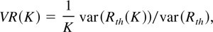
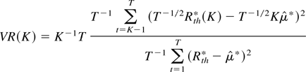
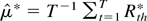
test is then to replace population variances by sampling variances. Let
Rth denote returns computed over one period
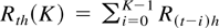
of length h, defining the sampling interval used, and
denote K-period returns; the variance ratio statistic is defined
by
where
.
It was applied to U.S. real gross national product (GNP) by Cochrane
(1986) and to financial assets by Poterba and
Summers (1988), Lo and Mackinlay (1989), and Faust (1988,
1992).
Lo and Mackinlay (1988, 1989) derive the basic asymptotic distributions for a
fixed K and provide an extensive simulation analysis of size and
power. They show important size distortions, and their results illustrate
the fact that power may be a nonmonotonic function of K.
Richardson and Smith (1991, 1994) analyze, among other things, asymptotic power
using the approximate slope function of Bahadur (1960) and Geweke (1981). A
similar approximate slope analysis is provided by Campbell (2001) in a related context (regression-based tests).
Faust (1992) shows that the variance ratio
statistic is approximately optimal for some class of alternatives (this
class varying with K). Daniel (2001)
uses a different asymptotic framework to analyze power whereby returns are
modeled as being locally uncorrelated (i.e., returns are independent and
identically distributed [i.i.d.] plus a stationary
autoregressive moving average [ARMA] process whose importance
vanishes at rate T1/4). As mentioned earlier,
Richardson and Stock (1989) use an asymptotic
framework whereby K/T → κ. They show that
the resulting asymptotic distribution provides a much improved
approximation to the finite sample distribution. Deo and Richardson (2003) show that under this asymptotic framework, the
variance ratio test is inconsistent. We shall comment on some of these
contributions throughout the paper. The bottom line is that our
continuous-time asymptotic framework retains the advantages of the
analysis of Richardson and Stock (1989) for size
but offers a much improved treatment of power.
The rest of this paper is structured as follows. Section 2 describes
the limit distribution of the variance ratio statistic under the null
hypothesis of market efficiency defined by uncorrelated returns. In
Section 3, we consider three alternative hypotheses of interest: (a) with
the dividend-price ratio as a predictor of returns (modeled as a
near-unit-root process); (b) with trend-stationary prices; and (c) with
prices as the sum of a permanent and transitory component. The limit
distribution of the statistic is derived for each case. Section 4 presents
simulation experiments to investigate the following issues: the adequacy
of our asymptotic distributions as approximations to the finite sample
distributions (under both the null and alternative hypotheses); and what
features influence the power of the test. Our results show, in particular,
that the power of the variance ratio statistic initially increases with an
increase in the aggregation parameter κ but subsequently decreases as
κ is increased further. This has important practical implications
because it indicates that for a given alternative hypothesis there is a
value of K relative to T that maximizes power. Section 5
investigates the properties of a test that is the maximal value of the
variance ratio over a range of possible values for K. Critical
values are provided, and we discuss how the trimming to define this range
affects power. Section 6 presents concluding remarks, and an Appendix
gives technical derivations.
2. LIMIT DISTRIBUTION UNDER THE NULL
HYPOTHESIS
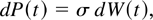
Under the null hypothesis, we consider the following continuous-time
stochastic process for P(t), the logarithm of the price
of an asset or a portfolio at time t:
with t ∈ [0,N] and P(0) =
Op(1), an arbitrary constant or a random
variable. The discrete-time representation of the process for a sampling
interval of length h is given by
where N is the span of the data, h is the sampling
interval, and εth is i.i.d.
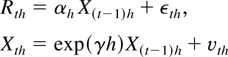
N(0,hσ2). We define returns over a period
of length h by Rth =
Pth −
P(t−1)h. Under the null
hypothesis, the discrete-time representation for returns is then
Note that the Gaussian assumption on the errors that follows from
taking a discrete-time approximation to a continuous-time model is not
restrictive. The same asymptotic results hold allowing a general class of
processes for the errors of the discrete-time model. What is needed are
conditions on the discrete-time errors such that the results stated in
Lemma A.1 in the Appendix hold. Such conditions can allow nonnormal
processes with some forms of heteroskedasticity. This holds true under
both the null and the class of alternative hypotheses to be considered
later.
2.1. Case with K Fixed
When K is fixed, Lo and Mackinlay (1988) and Faust (1988)
showed that the limiting distribution under the null hypothesis (3) is
Lo and Mackinlay (1989) considered the
adequacy of this normal asymptotic distribution as an approximation to the
finite sample distribution, in particular for the case where the data are
generated by (3). They showed the approximation to be adequate when
K is small and T is large but less so when K is
large. They also showed that the variance ratio test can have better power
than other tests under several alternatives (log-prices following an AR(1)
process, log-prices having both a permanent and a transitory component,
returns following an AR(1) process). Faust (1988) notes, however, that these power gains are
seriously undermarked by the presence of substantial size distortions that
increase as K increases. For example, when T = 732 and
for a nominal size of 5%, the exact size of the test is 1.6% for
K = 48, 0.06% for K = 72, and 0.0% for K =
120.
2.2. Case with K → ∞ and
K/T → κ
The simulation results discussed previously suggest that the
asymptotic normal approximation is inadequate when K is rather
large relative to the sample size T. Hence, we consider the
alternative asymptotic framework whereby K increases to infinity
and the ratio K/T tends to a limit κ (0 <
κ < 1). The limit distribution of the statistic
VR(K) under the null hypothesis is given in the
following proposition, proved in the Appendix.
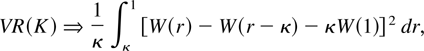
PROPOSITION 1. If K/T → κ and
K → ∞ as T → ∞ with 0 <
κ < 1 and N fixed, then under the null hypothesis (3), we
have
with W(r) a standard Wiener process.
The limit distribution (5) is the same as that derived by Richardson
and Stock (1989), who used a fixed h
asymptotic framework with K/T → κ as
T → ∞. Note that the limiting distribution depends on
the nuisance parameter κ.
3. LIMIT DISTRIBUTION UNDER SEVERAL
ALTERNATIVES
3.1. Alternative H1: Dividend-Price
Ratio as a Predictor
We consider two continuous-time stochastic processes,
P(t) denoting the logarithm of the price of an asset or
a portfolio and X(t) a variable such as the
dividend-price ratio. We let Z(t) =
(P(t),X(t))′ and assume that
Z(t) is generated by the diffusion process
with t ∈ [0,N] and Z(0) =
(P0,X0)′ =
Op(1),
and where W =
(W1,W2)′ is a
two-dimensional standard Wiener process with covariance
The solution to the stochastic differential equation (6) is (e.g.,
Arnold, 1974)
with
Assuming that Z(t) is observed over the time
interval [0,N], and defining the sampling interval
h by Th = N, we can obtain the exact
discrete-time representation Zth of
Z(t) that is given by the following autoregressive
process of order one:
where Zth =
(Pth,Xth)′,
Z0h = Z(0), and
The random component uth is i.i.d.
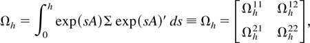
N(0, Ωh) with
where
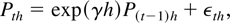
As before, returns over a sampling interval of length h are
given by Rth =
Pth −
P(t−1)h. Using the notation
uth =
(εth,vth)′ and
αh = β(exp(γh) −
1)/γ, we obtain from (9) the following discrete-time model for
returns and the dividend-price ratio:
for t = 1,…,T ≡
N/h and where uth =
(εth,vth)′
∼ i.i.d. N(0,Ωh).
For a fixed sampling interval, the system (10) implies that the
univariate process for returns, Rth, is an
ARMA(1,1), consistent with the idea that asset prices have permanent and
transitory components (e.g., Poterba and Summers,
1988; Campbell, 2001). It also implies
that conditional on information available at time t,
Ith, expected returns are given by
E(R(t+1)h|Ith)
= αh Xth.
Accordingly, expectations of future returns are affected by the
dividend-price ratio. Letting c = γN and g
= βN, we can write αh =
g(exp(c/T) − 1)/c ≃
g/T. Hence, in the asymptotic framework where
T → ∞ with N fixed, we can interpret
αh as a sequence of local alternatives with
noncentrality parameter g. Under these specifications, the limit
of the variance ratio statistic when K → ∞ and
K/T → κ as T → ∞ is
given in the following proposition, proved in the Appendix.
PROPOSITION 2. If K → ∞ and
K/T → κ with 0 < κ < 1,
when T → ∞ with N fixed, we have, under the
alternative H1,
with
. Also, W1(r) and
W2(r) are independent Wiener processes,
.
We consider, as in Lo and Mackinlay (1989),
the two-sided critical region defined by {VR(K) <
λ1 or VR(K) > λ2} where
λ1 and λ2 are constants. Denoting by
λα1(κ) and
λ1−α2(κ) the quantiles of order
α1 and 1 − α2 of the limit
distribution (5), the asymptotic power of a two-sided test with size μ
(α1 + α2 = μ) is given by, for any
g ≥ 0,
where L1(g,κ,c,δ) is the
limit distribution (11).
3.2. Alternative H2: Mean-Reverting
Prices
As a second alternative hypothesis of interest, we follow Shiller and
Perron (1985), among others, and suppose that
the logarithm of prices is a stationary Ornstein–Ühlenbeck
process:
with γ < 0, P(0) = P0, and
t ∈ [0,N]. We suppose, for simplicity,
that η = 0. The discrete-time representation is given by the
following AR(1) process, for t = 1,…,T ≡
N/h:
with P0h = P0 and
where εth ∼ i.i.d.
N(0,a(h)) with a(h) =
σ2(exp(2γh) − 1)/2γ.
Returns being defined as Rth =
Pth −
P(t−1)h, the limit
distribution, as T → ∞ with N fixed, of the
variance ratio statistic is given by, under this alternative
hypothesis,
where
.
Setting γ = 0, it is easily seen that the same null limiting
distribution obtains.
3.3. Alternative H3: Prices as the
Sum of Permanent and Transitory Components
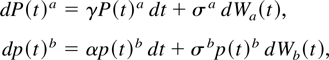
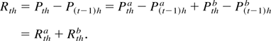
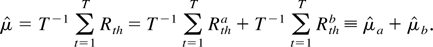
As a third alternative hypothesis of interest, we suppose that the
logarithm of prices is represented by the sum of two processes, namely, a
permanent component P(t)b and a
transitory component P(t)a. These
processes are specified as follows, for t ∈
[0,N]:
where p(t)b =
exp(P(t)b) is the level of the
permanent component of prices and
Wa(t) and
Wb(t) are two independent Wiener
processes. The initial values are P(0)a =
P0a and
P(0)b =
P0b. It is assumed that γ <
0 and, hence, that the transitory component,
P(t)a, is a stationary
Ornstein–Ühlenbeck process. The permanent component,
P(t)b, is a geometric Brownian
motion. The discrete-time representations are given by
with P0ha =
P0a,
P0hb =
P0b, and where
(uth,vth)′
∼ i.i.d. N(0,Ωh) with
We suppose for simplicity that α =
(σb)2/2 so that the permanent
component has no drift. Returns are defined by
Rth = Pth
− P(t−1)h where
Pth =
Ptha +
Pthb. The stochastic
process for returns is then an ARMA(1,1) similar to that considered by
Summers (1986), Poterba and Summers (1988), and Fama and French (1988a).
It is straightforward to show that the limit distribution of the
variance ratio statistic under H3, as T
→ ∞ with N fixed, is given by
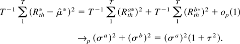
with
.
Under H0, γ = 0, and we recover the result of
Proposition 1.
Under the alternatives H2 and
H3, the critical regions are defined as for
H1. The asymptotic power of a two-sided test with
significance level μ is given by, for i = 2, 3,
with c ≤ 0, λα1(κ), and
λ1−α2(κ) being the quantiles of
order α1 and 1 − α2 (α1
+ α2 = μ) of the limit distribution (5) and
Li(κ,c,τ), i = 2,
3, the limit distribution under the relevant alternative
Hi, i.e., either (13) or (15). Under the
alternatives H2 and H3, power
depends on κ and c and the normalized initial value of the
transitory component P0a*. Under
H3, it also depends on τ, the square root of the
limit, as h converges to 0, of the relative variance of the
permanent and transitory components. As τ increases, the permanent
component becomes more important and the power approaches the size of the
test and vice versa.
3.4. Remarks on Consistency
In the asymptotic distributions presented previously, the relevant
noncentrality parameters that measure the distance between the null and
the alternative hypotheses are g = βN for
H1 and c = γN for
H2 and H3. Hence, the tests will
be consistent against these alternatives provided the span of the data
N increases as the sample size increases. Increasing the sample
size is not enough to ensure consistency of the test (see Perron, 1991). This is in contrast to the result of
Deo and Richardson (2003), who show that the
variance ratio statistic is inconsistent in the standard
K/T → κ asymptotic framework. The main
reason for the discrepancy is the ad hoc nature of the standard
K/T → κ asymptotic framework. As a result,
the noncentrality parameter that measures the distance between the null
and the alternative hypothesis is held fixed as the sample size increases,
irrespective of the span of the data or the sampling interval. Our
continuous-time asymptotic framework directly links the noncentrality
parameter as a function of the underlying continuous-time parameters and
the span of the data. Hence, it provides a more coherent framework to
analyze power. In light of this, the simulation results of Deo and
Richardson (2003) can be interpreted as
pertaining to the asymptotic power when T increases and
N, the span of the data, is held fixed. Hence, it is not
surprising that power does not increase to one for fixed alternatives.
4. SIMULATION EXPERIMENTS
The aim is first to present results pertaining to the power function
for various sample sizes and parameters and show that the asymptotic power
functions provide good approximations in moderate-sized samples. We then
highlight the effect of the aggregation parameter κ on the asymptotic
power. We do not discuss the adequacy of the asymptotic distribution (5)
under the null hypothesis. This was studied by Richardson and Stock (1989), who concluded that it indeed provides a good
approximation, far superior to the fixed K asymptotic
distribution examined by Lo and Mackinlay (1989); see Section 2.1.
We first consider the case where the initial values are set to zero.
The effects of nonzero values are assessed in Section 4.4. The exact
distributions under the null hypothesis are obtained for different values
of T using 10,000 simulations of the process (3). The exact power
functions are then computed simulating the exact distributions under the
various alternative hypotheses. The limiting distributions are also
obtained using simulations; quantities such as
J2(r) and W12(r)
are approximated by
,
respectively. The various integrals are constructed by the appropriate
normalized sums with T = 1,000, and
Xt =
exp(c/T)Xt−1 +
vt where ut and
vt are drawn independently from a
N(0,1). Other quantities are simulated in a similar fashion.
4.1. Finite Sample and Asymptotic Power
We now consider the finite sample power under the three alternatives
described before. To that effect, we use the following values of
N (the total horizon of the data) and T (the total
number of observations) with h = N/T
defining the sampling interval: N, T = 8, 16, 32, 64,
128, 256, 512, 1,024, 2,048, and ∞. The results are presented in
Tables 1, 2, and 3 for two-sided tests of nominal size 5% and values of
the aggregation parameter
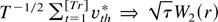
.
The values selected for the various parameters under the alternative
hypotheses are as follows. For H1, δ = 0, β =
0.1 and γ = −0.02; hence the regressor is mean-reverting and
affects returns in a positive way.
1 We also
performed the experiments with δ = −0.5 and −0.9 but do
not report the results explicitly though we shall comment on the
differences.
For
H2, γ = −0.2, and
prices are accordingly stationary. For
H3, the
transitory component is again generated with γ = −0.2 and τ
= ½ so that the noise of the transitory components dominates. The
values of the parameter γ are chosen to have a wide range of values
for power given the configurations for
N and
T (i.e.,
not all close to one or the size of the test). Note that the power for
alternative values of γ can be obtained from the tables. The relevant
parameter is of the form exp(γ
h), and a given diagonal
corresponds to a particular value of
h =
N/
T. Because
N and
T are doubled
across each row or column the power for γ* =
2
iγ can be obtained by looking at the entries
i diagonals below (
i > 0) or
i diagonals
above (
i < 0).
Power of VR(K) against H1: δ
= 0.0, β = 0.1, γ = −0.02
Power of VR(K) against H2: γ
= −0.2
Power of VR(K) against H3: γ
= −0.2, τ =
σb/σa =
½
In general, for any given value of κ, we observe the following
features: if N is small (N ≤ 16), the power is close
to the size; for a given fixed T, the power increases
substantially with N; for a given N, the increase in
power as T increases is important when T is small but
becomes marginal when T reaches 128 or 256. Power depends much
more on the span of the data than on the number of observations per se
(see also Shiller and Perron, 1985; Perron, 1991). A feature of substantial interest is
that, for any alternative considered, the power initially increases with
an increase in κ and subsequently decreases as κ increases
further. Results not shown indicate that, under H1, an
increase in |δ| reduces power but the asymptotic
distribution remains a good approximation. Similarly, under
H3, an increase in τ decreases power.
Overall, the results also show that the asymptotic power functions are
good approximations to the finite sample power unless the sample size is
small. The approximations are better when κ is small but still
adequate when κ is large.
4.1.1. Remarks on Alternative Approximations.
As discussed in Section 3.4, the standard K/T
→ κ asymptotic framework used by Richardson and Stock (1989) and Deo and Richardson (2003) is not adequate to analyze power. Another
popular approach to analyze the power function of tests is the so-called
Bahadur's slope approximation. In the context of the variance ratio
statistic, this was used by Richardson and Smith (1991). But this approach is tailored to assess
relative power performance between two tests; hence it cannot provide a
direct approximation to the power function for selected parameter
configurations (it can, however, be used to select a candidate value of
K that maximizes power; see Section 4.3). Our approach, on the
other hand, can provide a direct approximation to the power function, and
as we have shown it does provide a rather good approximation from which
reliable relative rankings can be obtained. This, we believe, shows the
usefulness of the asymptotic framework adopted.
4.2. Asymptotic Power as a Function of
κ
Using simulations with 2,000 replications, we obtained the asymptotic
power under H1, H2, and
H3 for κ = 0.00 … (0.02) … 0.70. For
H1, we set c = γN = −5 and
vary g = βN from 0 to 28 (in steps of 2). We also
consider δ = 0, −0.5, and −0.9. For
H2, we vary c = γN from 0 to
−28 (in steps of 2) whereas for H3, we set τ
= ½ and vary c from 0 to −80 (in steps of 4).
The results are presented in Figures 1,
2, and 3 and Table 4 summarizes the importance of κ for the
various experiments considered by presenting, for each case, the value of
κ that maximizes asymptotic power. The results show, as expected, that
the power is close to the size of the test when g is small, in
which case variations in κ have no important effect. When g
increases, variations in κ induce more important differences in power.
When δ = 0 or −0.5, the value of κ that yields maximal power
is smaller the more distant g is from the null value. When δ
= −0.9, the value of κ that yields maximal power initially
increases with an increase in g but eventually decreases with
further increases in g. The results also show that when
c = −5 (dividend-price ratio being locally stationary), the
test can be biased for alternatives g close to 0 and that this
bias increases as |δ| increases. In general, power
decreases with an increase in |δ| when c <
0.
Asymptotic power under H1: (a) c =
−5, δ = 0; (b) c = −5, δ = −0.5; (c)
c = −5, δ = −0.9. (Figure continues on next
page.)
Asymptotic power under H2: τ = 0.
Asymptotic power under H3: τ = ½.
Values of κ that maximize power for selected
alternatives
The alternatives H2 and H3
allow us to analyze the joint effect of c and κ on the power
of the test. Given that, here, c measures the extent to which
log-prices are far from being a random walk, Figure
2 shows that, for H2, the faster prices revert
to their mean value (c more negative), the stronger is the effect
of variations in κ on power. Remarkably, a value of κ = 0.22
yields maximal power for all values of c considered. Under the
alternative H3, the power is again substantially
affected by κ. As for H1, the value of κ that
yields maximal power decreases as the alternative gets further away from
the null.
To summarize, the asymptotic distributions obtained with
K/T → κ provide adequate approximations to
the finite sample distributions under both the null hypothesis and the
three alternatives selected. A salient feature of the power function under
all these alternatives is that power initially increases and then
decreases as κ increases, which accords with the simulation results of
Lo and Mackinlay (1989).
4.3. Comparison with Bahadur's Approximate Slope
Function
An alternative approach that delivers a prediction about the value of
K that maximizes power is the approximate slope function
developed by Bahadur (1960) and extended by
Geweke (1981). When the limit distribution of a
statistic is chi square under the null hypothesis (as is the square of the
variance ratio statistic under the standard asymptotic framework), then
the approximate slope equals the probability limit of the statistic under
the alternative hypothesis deflated by the sample size. Among
asymptotically valid statistics, the one with a maximal approximate slope
is predicted to have better power. Richardson and Smith (1991) used this approach to analyze the value of
K that would maximize the power of the variance ratio statistic
in the context of an AR(1) alternative as specified by our alternative
H2. In this section, we revisit the analysis and
results underlying their Table 7. They showed that when the alternative is
an autoregressive parameter 0.95 (= exp(γh) in our notation),
Bahadur's approximation suggests that K = 48 will maximize
power, this value being the same for all sample sizes. In contrast, our
approach suggests that a value of K = 0.22T will
maximize power.2
An autoregressive parameter
0.95 with T = 720 implies a value of γ = −37,
approximately. Although this value is outside the range of Table 4, we
have verified that the value of κ that maximizes power is still
0.22.
We replicated Richardson and Smith's (1991) experiment with T = 720 (as they did)
and T = 360 also. For reasons that will become clear, we evaluate
power using (1) the standard normal critical values suggested by the usual
fixed K asymptotic framework and (2) the critical values from the
asymptotic framework in which K/T → κ. The
results are presented in Table 5. As can be seen
from the first column, when T = 720 the approximate slope does
well in selecting the value of K that maximizes power when the
fixed K asymptotic critical values are used.3
The power entries in the first column of Table 5 are higher
than those reported in Table 7 of Richardson and Smith (1991) for reasons unknown to us. Nevertheless, the
shape of the power function is generally the same, and the same
conclusions follow.
Because these imply tests with large size
distortions when
K is large (too conservative), it can be said to
perform well with non-size-adjusted power. However, from the results in
the second column, it is seen to be very sensitive to the sample size
used. Changing the sample size to
T = 360, a value
K =
48 yields very low power (compared to the highest possible at
K =
24).
Finite sample power, alternative H2,
exp(γh) = 0.95
Things are very different when evaluating power with critical values
from the K/T → κ asymptotic framework,
which is basically equivalent to analyzing size-adjusted power because the
tests then have very little size distortion. When T = 720, our
approach suggests that K = 158 will maximize power, which is
indeed the case. The power is 0.97 compared to 0.85 when K = 48
is selected. More important, our approach is robust to changes in the
sample size. When T = 360, our framework predicts that K
= 79 will maximize power, which is close to the maximum attainable.
From these simulations, we can conclude that our approach is better
suited than the slope approximation to provide a value of K that
will maximize power, provided the K/T → κ
asymptotic critical values are used, which should be done in any event to
avoid highly size-distorted tests.
4.4. The Effect of Nonzero Initial Conditions
We now consider the effect of a nonzero initial value on the power of
the test under the different alternatives (the size is unaffected because
the statistic is invariant to the initial value under the null
hypothesis). To illustrate the qualitative results, we consider the
alternatives H1 with c = −5 and δ =
0, and also H2 and H3 with τ =
½. We simulated the power function of the variance ratio statistic
for values of the normalized initial conditions between 0 and 6. The
results are presented in Figure 4.
Effect of a nonzero initial value on asymptotic power.
The results show that, in general, a nonzero initial value increases
the power of the test. This increase is bigger the further away prices are
from being a random walk. This result is fairly intuitive. When prices
have a stationary component, the larger the initial value the further away
from the unconditional mean is the process at time 0. Hence, the movement
at the beginning shows a strong reversion to the mean, the reversion
appearing stronger the larger the initial value. When prices have an
explosive component, the effect of a nonzero initial value is to
exacerbate the speed at which the process departs from its initial value.
Hence, it becomes even easier to distinguish from a random walk.
There are some exceptions that show that the power can initially
decrease with an increase in the initial value. This occurs, most notably,
when prices are strongly mean-reverting (alternative
H2 with a large negative c). This is due to
the fact that a nonzero initial value has the effect of increasing the
variance ratio whether the process is mean-reverting or explosive. With a
mean-reverting process, the variance ratio take values below one, and we
reject for small values. Hence, this increase causes a decrease in power.
Eventually, as the initial value gets larger the mean reversion effect
dominates.
5. A TEST THAT DOES NOT DEPEND ON
κ
The fact that the power function of the variance ratio statistic for
alternatives of interest attains a maximum for some value of κ means
that power losses can be important if κ is not chosen appropriately.
The value of κ that maximizes power depends, however, on the
underlying true data-generating process under the alternative hypothesis,
which is unknown. Hence, a useful strategy is to look at the variance
ratio statistic over a range of values for κ. To motivate the approach
adopted consider first the case where the alternative is right-sided,
i.e., we reject for large values of the variance ratio statistic. A common
strategy is to find the value of κ that leads to the strongest
possible rejection. This leads to the test statistic
VRmax =
supκ∈[ε,1−ε]
VR([Tκ]), which looks for the maximal
value of the variance ratio statistic. Here, ε is some trimming
parameter that defines the range of permissible values for κ. Applying
the same logic to the case of left-sided alternatives (rejecting for low
values of the statistics) would lead us to consider the minimal value of
the variance ratio statistic over some range for κ. This approach,
however, leads to a test with no power because the distribution of
VR(K), both in finite samples and asymptotically, has
some mass at 0. Hence, the distribution of the minimal value has a rather
important mass at 0, and the critical values (using standard significance
levels) are basically 0. Because the statistic is bounded below by 0, this
implies basically no power. For this reason, we continue to consider the
VRmax statistic even for left-sided alternatives. The
interpretation is then that one is looking at the least favorable case for
the alternative and whether it still implies a rejection. Hence, for
left-sided alternatives, it should be viewed as a conservative
procedure.4
As suggested by a referee, it
would be possible to use a cross-validation procedure to select the best
value of κ. Such an extension is not reported here.
Using the result of Proposition 1, the asymptotic distribution of
VRmax is
Table 6 presents the quantiles of the
asymptotic distribution and also those of the finite sample distributions
for selected values of T and ε. Two features of interest
are noteworthy from these results. First, the asymptotic distribution is,
in general, a good approximation to the finite sample distributions.
Second, changing ε has little effect on the quantiles of the
distribution in the right tail but substantial effects in the left tail.
This suggests that different values of ε are unlikely to affect the
power of the test when the alternative is such that the variance ratio
increases above 1. However, the choice of ε could substantially
affect power when the alternative is such that the variance ratio
decreases below 1.
Quantiles of the distribution of
maxκ∈[ε,1−ε]VR([Tκ])
under H0
To assess the extent of the potential power losses compared to that
attainable with the “best” κ, we simulated the asymptotic
power function of the test VRmax when the alternative
is either H1 or H2. Consider first
the asymptotic power function when the alternative is
H1 with c = δ = 0 (Figure 5). Here returns are influenced by the
dividend-price ratio, which is modeled as a nearly integrated process.
This is a case in which the variance ratio statistic takes values above 1
(increasing as the sample size increases). As expected, the power function
is basically invariant to the value of the trimming used. It is somewhat
below that attainable with the best fixed κ but substantially above
that obtained with other possible choices for κ. Hence, the test
provides a useful way to deal with the fact that the best κ is unknown
in practice while retaining reasonable power.
Asymptotic power function of VRmax: alternative
H1.
Consider now the case when the alternative is H2
(Figure 6). Here prices are stationary, which
causes the variance ratio to take values below 1 (approaching 0 as
T increases). The power function is now severely affected by the
choice of the trimming value ε. Indeed, power decreases as ε
approaches 0. This is due to the fact that when K = 0,
VR(K) = 1 by definition. Hence, for small values of the
trimming the maximal value of VR(K) has to be, basically
by construction, close to 1; hence, the associated power loss.
Asymptotic power function of VRmax: alternative
H2.
Because the trimming is inconsequential for the right-sided
alternative and a moderate to large trimming is preferable for the
left-sided alternative, a sensible strategy is to use a trimming in the
range 0.10 to 0.20.
6. CONCLUSION
We considered a test of market efficiency based on the variance ratio
statistic. Our framework was to posit a continuous-time process of
interest, derive its discrete-time representation, and then take the limit
as the sample size T increases, keeping the span of the data
fixed (i.e., letting the sampling interval tend to zero at rate
T). We described the limit distribution of the variance ratio
statistic under the null hypothesis of market efficiency defined by
uncorrelated returns and under three alternative hypotheses of interest:
namely, with the dividend-price ratio as a predictor of returns, with
trend-stationary prices, and with prices as the sum of a permanent and
transitory component. Simulations have shown that the limiting
distributions obtained are good approximations to the finite sample
distributions. An analysis of the power functions showed that, under all
alternatives considered, an increase in the aggregation parameter κ
induces an initial increase in power followed by a decrease as κ is
increased further. Hence, for a given alternative hypothesis there is a
value of K relative to T that maximizes power. This is
contrary to regression-based tests, e.g., regressing K-period
returns on the dividend-price ratio (see, e.g., Fama
and French, 1988b), in which case Perron and Vodounou (2004) showed that power decreases monotonically as
κ increases. For that reason, we have also considered the
VRmax test, which looks at the maximal value of the
variance ratio statistic over a prespecified range for K. We have
shown that this leads to a test with power close to that attainable with
the “best” value of κ. We have also shown that care must
be exercised in choosing the trimming that defines the range of values for
K considered and that a very small trimming should be
avoided.
APPENDIX: PROOF OF PROPOSITIONS 1 AND
2
The statistic VR(K) being invariant to linear
transformation of Rth, we use the normalized
process Zth* =
Zth /h1/2.
Throughout, we make extensive use of the following results, which are now
standard.
LEMMA A.1. Let uth =
(εth*,vth*)′ =
(εth,vth)′/h1/2
be i.i.d. (0,Σ) with Σ defined by (7).
Then, (i)
;
(ii)
(jointly) where W1(r) and
W2(r) are independent Wiener processes
defined on C[0,1] and ⇒ denotes weak
convergence in distribution. Also, (iii)
.
To obtain the limit distribution of VR(K) under
H1, we first consider the following lemma related to
sample moments.
LEMMA A.2. Let
(Rth,Xth,eth)
be generated by (10) and
(Rth*,Xth*,eth*)
=
(Rth,Xth,eth)/h1/2.
Also, let g = βN and T = N/h; then as
T → ∞ with N fixed, we have, with
,
Proof. Using Lemma A.1, we have, for part (i),
For part (ii)
For part (iii)
because (ah /h) →
β. The variance ratio statistic can be written as
with
.
For the denominator, we have
using Lemma A.1(iii), because
(see the discussion that follows) and
.
For the numerator, we have
because
The result of Proposition 2 follows. The limit distribution under the
null hypothesis (Proposition 1) is obtained setting β = 0 (hence,
g = 0) and noting that the marginal distribution of
W12(r) is that of a standard Wiener process.
█
Proof of (13). We use the normalized process
where Pth* =
Pth
/a(h)1/2 and
εth* = εth
/a(h)1/2. Because
,
we only consider the limit of the numerator. We first have
using c = γN and
a(h)/h → σ2. From this
result we deduce that
from which equation (13) follows. █
Proof of (15). We start by noting that
Hence, returns are the sum of the “permanent” and
“transitory” returns. We also define
Using the preceding notation, we can express the numerator, normalized
by h1/2, as
Now,
R[Tr]h*([Tκ])a
are returns corresponding to stationary mean-reverting prices; hence we
can apply the results corresponding to H2. Similarly,
R[Tr]h*([Tκ])b
are returns corresponding to random walk prices; hence we can apply the
results corresponding to H0. We then have the
following limit:
where W(r) =
Wb(r) +
τWa(r) with τ =
σb /σa. Next, we check
the denominator.
The proof of (15) follows. █