Numerical Simulations on the Motions of Anchored Capesize Ships

Youjia Zou; Chun Shen; Xiangying Xi

doi:10.1017/S0373463311000580

Numerical Simulations on the Motions of Anchored Capesize Ships

Published online by Cambridge University Press: 25 November 2011

Youjia Zou ,

Chun Shen and

Xiangying Xi

Show author details

Youjia Zou*: Affiliation:
(Merchant marine college, Shanghai Maritime University, Shanghai, China)
Chun Shen: Affiliation:
(Merchant marine college, Shanghai Maritime University, Shanghai, China)
Xiangying Xi: Affiliation:
(Faculty of Management, Wuhan University of Technology, Wuhan, China)
*: (E-mail: marscar@126.com)

Article contents

Abstract
INTRODUCTION
MODELING OF THE NONLINEAR MOTIONS
MODELING THE CHAIN TENSION AND ANCHOR HOLDING FORCE
NUMERICAL SIMULATIONS
VALIDATION OF THE SIMULATION RESULTS
ANALYSIS OF SIMULATION AND MODEL TEST RESULTS
CONCLUSIONS
References

Rights & Permissions

Abstract

When a ship is moored by a single anchor at the anchorage, its combined motions (i.e. yaw, sway, surge, etc.) are usually induced by external forces. Previous studies have gained some insights into the forces on anchor chains, but the motions for Capesize vessels still need to be further investigated. The length of anchor chain required for safe anchoring also needs to be carefully calculated rather than determined solely by the experience and judgement of Captains. The relationship between the length of chain and water depth, wind force, current velocity and the trim (draught difference forward/aft) requires further study. Our new methods consider all necessary factors which may exert significant influence on ships, including not only the water depth at the anchoring location but also the particulars of the ships, its equipment and the environmental conditions. Here, a numerical simulation model to describe the behaviour of an anchored Capesize ship is presented, with the comparison of results between simulations and real time model tests carried out. A discussion highlights the important features of the methods which provide mariners with theoretical solutions.

Keywords

Numerical simulation Length of chain Period Amplitude

Type: Research Article
Information: The Journal of Navigation , Volume 65 , Issue 1 , January 2012 , pp. 145 - 158

DOI: https://doi.org/10.1017/S0373463311000580 [Opens in a new window]
Copyright: Copyright © The Royal Institute of Navigation 2011

1. INTRODUCTION

A ship at anchor is subject to wind, current and waves. The steady wind, current and wave drift forces induce a mean offset. The time-dependent wave drift forces can cause a low frequency slow drift motion around this mean offset and the first order wave forces generate the wave frequency vessel motions around the low frequency excursions (Biguang Hong, Reference Biguang1989). Because of limited restoring forces in yaw and sway directions, in the case of a single anchor, these motions can have considerable amplitudes and may therefore generate additional loads at the anchor and the chain stopper. This unstable behavior may trigger fishtailing movements where the vessel experiences large sway and yaw motions with periods even longer than the low frequency surge motions (Kim et al., Reference Kim, Ran and Zheng2001). However, a proper length of anchor chain for a Capesize vessel can provide more lateral stability due to friction forces arising from horizontal movement of the chain over the sea bottom.

The safety of the ship at an anchorage requires precise knowledge of anchoring operations especially for Capesize ships, which are affected by water depth, bottom natures, characteristics of the anchor and chain, vessel conditions, hydrodynamic interactions, and environmental conditions such as wind, wave or current (Sariöz and Narli, Reference Sariöz and Narli2003). Previous analytical techniques need to be further developed to quantitatively and qualitatively depict the motions of large ships while anchoring. A well established and proven numerical simulation study is considered to be the most reliable method for such a purpose. In this paper, a computer aided ship numerical simulation procedure (Fossen, Reference Fossen1994; Godhavn et al., Reference Godhavn, Fossen and Berge1998) and construction of state space equations are used and developed to simulate the motions of Capesize ships. The results of the simulations are also compared to the actual observations conducted for a 180,000 Dead Weight Tonnage (DWT) Capesize ship with a full load, anchored by means of a single anchor (port side) at a water depth of 35·6 m at Qingdao anchorage. The program calculates the external environmental forces and solves the nonlinear equations of motions in the time domain.

2. MODELING OF THE NONLINEAR MOTIONS

The basic mathematical model to represent the motions of a Capesize ship in the presence of wind and current consists of a set of non-linear state equations in six degrees of freedom; the three components of the velocity U(u, ν, w), and the three components of the angular velocity Ω(γ, p, q) (Klaka et al., Reference Klaka, Krokstad and Renilson2003). The Earth-fixed and ship (moving) coordinate systems are shown in Figure 1.

Figure 1. Global and Ship Coordinate System.

The ship's centre of gravity is located at (x _G, y_G, 0) in the system of coordinates. In order to simplify the problem it can be assumed that the principal axes of inertia of the ship are parallel to the chosen axis system, that the ship is symmetric about its centreplane, heave and pitch are not apparent, and roll angles are quite small for a Capesize ship (Sariöz and Narli, Reference Sariöz and Narli2003). The unique features of the Capesize ships allow us to make some assumptions that will reduce the number of degrees of freedom to three and the equations of the motions can be written as (Fossen, Reference Fossen1994):

(1)

$\dot \xi = \Phi (\xi )\nu$

(2)

$\dot \nu = H_1 \xi + H_2 \nu + H_3 \tau$

where H ₁ is the state matrix of the Earth-fixed positions and yaw angle ψ of the vessel, H ₂ is the state matrix of the body-fixed velocities, and H ₃ is the state matrix of the impact force and moment which are provided by external forces.

(3)

$\Phi (\xi ) = \left[ {\matrix{ {\cos (\psi )} & { - \sin (\psi )} & 0 \cr {\sin (\psi )} & {\cos (\psi )} & 0 \cr 0 & 0 & 1 \cr}} \right]$

is the rotation matrix in yaw and

(4.1)

$H_1 \equiv - N^{ - 1} T \equiv \left[ {\matrix{ {h_{1_{11}}} & {h_{1_{12}}} & {h_{1_{13}}} \cr {h_{1_{21}}} & {h_{1_{22}}} & {h_{1_{23}}} \cr {h_{1_{31}}} & {h_{1_{32}}} & {h_{1_{33}}} \cr}} \right]$

(4.2)

$H_2 \equiv - N^{ - 1} Q \equiv \left[ {\matrix{ {h_{2_{11}}} & {h_{2_{12}}} & {h_{2_{13}}} \cr {h_{2_{21}}} & {h_{2_{22}}} & {h_{2_{23}}} \cr {h_{2_{31}}} & {h_{2_{32}}} & {h_{33}} \cr}} \right]$

(4.3)

$H_3 \equiv N^{ - 1} \equiv \left[ {\matrix{ {h_{3_{11}}} & {h_{3_{12}}} & {h_{3_{13}}} \cr {h_{3_{21}}} & {h_{3_{22}}} & {h_{3_{23}}} \cr {h_{3_{31}}} & {h_{3_{32}}} & {h_{3_{33}}} \cr}} \right]$

The Earth-fixed positions (x, y) and yaw angle ψ of the ships is expressed in vector ξ=[x y ψ]^T. The body-fixed velocities are represented by the vector ν=[u ν γ]^T, where the elements in these state vectors describe the surge, sway and yaw modes, respectively (Wenjerchang et al., Reference Wenjerchang and Yilin2002). The impact force and moment are provided by the external forces, τ=[τ ₁τ ₂τ ₃]^T. N, Q and Γ are a set of matrices for a floating Capesize ship, see (Fossen, Reference Fossen1994) for details. Starboard-port symmetry of ships implies that N and Q are constructed as follows:

(5)

$$N = \left[ {\matrix{ {n_{11}} & 0 & 0 \cr 0 & {n_{22}} & {n_{23}} \cr 0 & {n_{32}} & {n_{33}} \cr}} \right],\;Q = \left[ {\matrix{ {q_{11}} & 0 & 0 \cr 0 & {q_{22}} & {q_{23}} \cr 0 & {q_{32}} & {q_{33}} \cr}} \right]$

N is the inertia matrix including hydrodynamic added inertia and moment. In general N will be nonsymmetrical, that is n ₂₃≠n ₃₂ due to the properties of hydrodynamic added inertia (Fossen, Reference Fossen1994). Q is the damping matrix, which is nonsymmetrical in most cases (Chakrabarti, Reference Chakrabarti2001).

The anchor forces and moment are usually described by a diagonal matrix as follows:

(6)

$\Gamma = \left[ {\matrix{ {\,f_{11}} & 0 & 0 \cr 0 & {\,f_{22}} & 0 \cr 0 & 0 & {\,f_{33}} \cr}} \right]$

After combining (1) and (2) in the space of state variables, we can obtain the following state equations (Wenjerchang et al., Reference Wenjerchang and Yilin2002):

(7.1)

$\dot x_1 = \cos (x_3 )x_4 - \sin (x_3 )x_5$

(7.2)

$\dot x_2 = \sin (x_3 )x_4 - \cos (x_3 )x_5$

(7.3)

$\dot x_3 = x_6$

(7.4)

$\eqalign{ \dot x_4 =& h_{1_{11}} x_1 + h_{1_{12}} x_2 + h_{1_{13}} x_3 + h_{2_{21}} x_4 + h_{2_{12}} x_5 \cr & + h_{2_{13}} x_6 + h_{3_{11}} u_1 + h_{3_{12}} u_2 + h_{3_{13}} u_3}$

(7.5)

$\eqalign{\dot x_5 = & h_{1_{21}} x_1 + h_{1_{22}} x_2 + x_{1_{23}} x_3 + h_{2_{21}} x_4 + h_{2_{22}} x_5 \cr & + h_{2_{23}} x_6 + h_{3_{21}} u_1 + h_{3_{22}} u_2 + h_{3_{23}} u_3}$

(7.6)

$\eqalign{ \dot x_6 = & h_{1_{31}} x_1 + h_{1_{32}} x_2 + h_{1_{33}} x_3 + h_{2_{31}} x_4 + h_{2_{32}} x_5 \cr & + h_{2_{33}} x_6 + h_{3_{31}} u_1 + h_{3_{32}} u_2 + h_{3_{33}} u_3}$

where:

(8)

$x(t) = [x_1 \ x_2 \ x_3 \ x_4 \ x_5 \ x_6 ]^T = [x \ y \ \psi \ u \ \nu \ r]^T$

(9)

$u(t) = [u_1 \ u_2 \ u_3 ]^T = [\tau _1 \ \tau _2 \ \tau _3 ]^T$

If assuming that yaw angle varies in a range of – ${\textstyle{\pi \over 2}}$ and + ${\textstyle{\pi \over 2}}$ , then above nonlinear equations can be rewritten as follows (Fossen and Grovlen, Reference Fossen and Grovlen1998):

$\dot x(t) = A_1 x(t) + B_1 u(t) \ {\rm if} \ x_3 \ {\rm is \ about \ 0,}$

$\dot x(t) = A_2 x(t) + B_2 u(t) \ {\rm if} \ x_3 \ {\rm is \ about} \ \displaystyle{\pi \over 2},\left({\left| {x_3} \right| < \displaystyle{\pi \over 2}}\right)$

$\dot x(t) = A_3 x(t) + B_3 u(t) \ {\rm if} \ x_3 \ {\rm is \ about} \ - \displaystyle{\pi \over 2},\left({\left| {x_3} \right| < \displaystyle{\pi \over 2}}\right)$

where:

$A_1 = \left[ {\matrix{ 0 & 0 & 0 & 1 & { - \alpha} & 0 \cr 0 & 0 & 0 & \alpha & 1 & 0 \cr 0 & 0 & 0 & 0 & 0 & 1 \cr {h_{1_{11}}} & {h_{1_{12}}} & {h_{1_{13}}} & {h_{2_{11}}} & {h_{2_{12}}} & {h_{2_{13}}} \cr {h_{1_{21}}} & {h_{1_{22}}} & {h_{1_{23}}} & {h_{2_{21}}} & {h_{2_{22}}} & {h_{2_{23}}} \cr {h_{1_{31}}} & {h_{1_{32}}} & {h_{1_{33}}} & {h_{2_{31}}} & {h_{2_{32}}} & {h_{2_{33}}} \cr}} \right]$

$A_2 = \left[ {\matrix{ 0 & 0 & 0 & \beta & { - 1} & 0 \cr 0 & 0 & 0 & 1 & \beta & 0 \cr 0 & 0 & 0 & 0 & 0 & 1 \cr {h_{1_{11}}} & {h_{1_{12}}} & {h_{1_{13}}} & {h_{2_{11}}} & {h_{2_{12}}} & {h_{2_{13}}} \cr {h_{1_{21}}} & {h_{1_{22}}} & {h_{1_{23}}} & {h_{2_{21}}} & {h_{2_{22}}} & {h_{2_{23}}} \cr {h_{1_{31}}} & {h_{1_{32}}} & {h_{1_{33}}} & {h_{2_{31}}} & {h_{2_{32}}} & {h_{2_{33}}} \cr}} \right]$

$A_3 = \left[ {\matrix{ 0 & 0 & 0 & \beta & 1 & 0 \cr 0 & 0 & 0 & { - 1} & \beta & 0 \cr 0 & 0 & 0 & 0 & 0 & 1 \cr {h_{1_{11}}} & {h_{1_{12}}} & {h_{1_{13}}} & {h_{2_{11}}} & {h_{2_{12}}} & {h_{2_{13}}} \cr {h_{1_{21}}} & {h_{1_{22}}} & {h_{1_{23}}} & {h_{2_{21}}} & {h_{2_{22}}} & {h_{2_{23}}} \cr {h_{1_{31}}} & {h_{1_{32}}} & {h_{1_{33}}} & {h_{2_{31}}} & {h_{2_{32}}} & {h_{2_{33}}} \cr}} \right]$

$B_1 = B_2 = B_3 = \left[ {\matrix{ 0 & 0 & 0 & {h_{3_{11}}} & {h_{3_{21}}} & {h_{3_{31}}} \cr 0 & 0 & 0 & {h_{3_{12}}} & {h_{3_{22}}} & {h_{3_{32}}} \cr 0 & 0 & 0 & {h_{3_{13}}} & {h_{3_{23}}} & {h_{3_{33}}} \cr}} \right]$

In which α=sin(2°) and β=cos(88°). Above can be represented as:

(10)

$\dot x(t) = \displaystyle{{\sum\nolimits_{i = 1}^3 {\omega _i [A_i x(t) + B_i u(t)]}} \over {\sum\nolimits_{i = 1}^3 {\omega _i}}}$

where:

$\omega _i (t) = \prod\limits_{\,j = 1}^6 {M_{ij}} (x_j (t))$

and M _ij(x _j(t)) is the grade of the membership of x _j(t) in M _ij, ω_i(t) is the weight of the i-th rule and it is appropriate for membership values. See (Fossen, Reference Fossen1994) for details.

3. MODELING THE CHAIN TENSION AND ANCHOR HOLDING FORCE

In order to better describe the motions and mooring loads of an anchored Capesize ship subject to wind and current, the low frequency motions (neglecting the high frequency motions) and the behaviour of the mooring chain must be determined. So, other models have also been exploited as follows (Heshu Liao et al., Reference Heshu, Weiqing and Baochun1995).

(11)

$\left. \matrix{F_x = F_p \cos (\phi - \theta ) \hfill \cr F_y = F_p \sin (\phi - \theta ) \hfill \cr M = F_p L_{hg} \sin (\phi - \theta ) \hfill} \right\}$

(12)

${\rm and} \ F_a = \lambda _a w_a + \lambda _c w_{cl} L_s$

where:

F _p - is the horizontal component of chain tension.
F _a - is the anchor holding force.
φ - is the ship heading.
θ - is the chain leading.
L _hg - is the distance from hawse pipe to the centre of gravity.
w _a - is the anchor mass in water, w _cl - is the chain mass lying at seabed, λ _a - is the anchor holding factor ranging from 3·5 to 6, λ _c - is the chain friction coefficient varying from 0·6 to 3·5 (Jiachang Yang et al., Reference Jiachang, Zuochang and Yuyang2005), L _s - is the length of chain lying at seabed.

For the chain tension, the catenary curve equation is used by the following expression (Jaroslaw, Reference Jaroslaw2003):

(13)

$F_T = \left( {d_h - 2\displaystyle{{F_T} \over {m_w}} sh^{ - 1} \left( {\displaystyle{{m_w L_k} \over {2F_T}}} \right)} \right)\displaystyle{{L_c} \over {L_k}}$

where:

d _h - is the distance from hawse pipe to anchored point, m _w - is the unit chain mass, L _k - is the length of chain hanging, L _c - is the length of chain.

In this numerical simulation, only the condition that the partial anchor cable is hanging is considered under the influence of wind and current.

4. NUMERICAL SIMULATIONS

In this paper, the concepts of nonlinear controller design have been employed for the motions. Therefore, Equations (3)∼(10) can be conveniently transformed into Linear Matrix Inequalities (LMI). Applying the interior point polynomial method (Nesterov and Nemirovski, Reference Nesterov and Nemirovski1994), we can find the solutions of LMI. The interior point polynomial method has been used to construct a useful package in the LMI-toolbox of MATLAB software (Boyd et al., Reference Boyd, Ghaoui, Feron and Balakrishnan1994).

We also took advantage of the datasets extracted from the experiments; although the added mass and inertia moment for regular objects can be obtained by theoretical calculations, it is only through an empirical method that this can be achieved for irregular objects such as ships (Xiuheng Wu, Reference Xiuheng1999).

$\eqalign{\displaystyle{{m_x} \over m} = & \displaystyle{1 \over {100}}\left[ {0{\cdot}398 + 11{\cdot}97C_b \left( {1 + 3{\cdot}73\displaystyle{d \over B}} \right) - 2{\cdot}89C_b \displaystyle{L \over B}\left( {1 + 1{\cdot}13\displaystyle{d \over B}} \right)} \right. \cr & \left. { + 0{\cdot}175C_b \left( {\displaystyle{L \over B}} \right)^2 \left( {1 + 0{\cdot}541\displaystyle{d \over B}} \right) - 1{\cdot}107\displaystyle{L \over B}\displaystyle{d \over B}} \right] \cr \displaystyle{{m_y} \over m} = & 0{\cdot}882 - 54C_b \left( {1 - 1{\cdot}6\displaystyle{d \over B}} \right) - 0{\cdot}156\displaystyle{L \over B}(1 - 0{\cdot}673C_b ) \cr & + 0{\cdot}862\displaystyle{L \over B}\displaystyle{d \over B}\left( {1 - 0{\cdot}678\displaystyle{d \over B}} \right) - 0{\cdot}638C_b \displaystyle{L \over B}\displaystyle{d \over B}\left( {1 - 0{\cdot}669\displaystyle{d \over B}} \right) \cr \sqrt {\displaystyle{{J_{zz}} \over m}} = & \displaystyle{L \over {100}}\left[ {33 - 76{\cdot}85C_b (1 - 0{\cdot}784C_b ) + 3{\cdot}43\displaystyle{L \over B}(1 - 0{\cdot}63C_b )} \right]}$

where

m _x - is the added mass about axes x.
m _y - is the added mass about axes y.
J _zz - is the added inertia moment.
m - is the mass of ship.
L/B - is the length between perpendiculars – breadth ratio.
d/B - is the depth – breadth ratio.
C _b - is the block coefficient.

The main particulars of the ship and the chain are given in Table 1.

Table 1. Main particulars of the ship.

The numerical simulations for above nonlinear equations are now presented. We consider the Capesize ship with system matrices as follows after processing the datasets (Godhavn et al., Reference Godhavn, Fossen and Berge1998):

$$\eqalign{& N = \left[ {\matrix{ {3{\cdot}806} & 0 & 0 \cr 0 & {5{\cdot}012} & { - 0{\cdot}682} \cr 0 & { - 0{\cdot}682} & {2{\cdot}327} \cr}} \right],Q = \left[ {\matrix{ {0{\cdot}072} & 0 & 0 \cr 0 & {0{\cdot}063} & {0{\cdot}013} \cr 0 & {0{\cdot}013} & {0{\cdot}005} \cr}} \right] \cr & \Gamma = \left[ {\matrix{ {5{\cdot}216} & 0 & 0 \cr 0 & {2{\cdot}397} & 0 \cr 0 & 0 & 0 \cr}} \right]}$

Then, the system matrices of the numerical model have the following forms:

$A_1 = \left[ {\matrix{ 0 & 0 & 0 & 1 & { - 0{\cdot}058} & 0 \cr 0 & 0 & 0 & {0{\cdot}058} & 1 & 0 \cr 0 & 0 & 0 & 0 & 0 & 1 \cr { - 0{\cdot}132} & 0 & 0 & { - 0{\cdot}252} & 0 & 0 \cr 0 & { - 0{\cdot}081} & 0 & 0 & { - 0{\cdot}264} & { - 0{\cdot}466} \cr 0 & { - 0{\cdot}226} & 0 & 0 & { - 0{\cdot}438} & { - 0{\cdot}513} \cr}} \right]$

$A_2 = \left[ {\matrix{ 0 & 0 & 0 & {0{\cdot}058} & { - 1} & 0 \cr 0 & 0 & 0 & 1 & {0{\cdot}058} & 0 \cr 0 & 0 & 0 & 0 & 0 & 1 \cr { - 0{\cdot}132} & 0 & 0 & { - 0{\cdot}252} & 0 & 0 \cr 0 & { - 0{\cdot}081} & 0 & 0 & { - 0{\cdot}264} & { - 0{\cdot}466} \cr 0 & { - 0{\cdot}226} & 0 & 0 & { - 0{\cdot}438} & { - 0{\cdot}513} \cr}} \right]$

$A_3 = \left[ {\matrix{ 0 & 0 & 0 & {0{\cdot}058} & 1 & 0 \cr 0 & 0 & 0 & { - 1} & {0{\cdot}058} & 0 \cr 0 & 0 & 0 & 0 & 0 & 1 \cr { - 0{\cdot}132} & 0 & 0 & { - 0{\cdot}252} & 0 & 0 \cr 0 & { - 0{\cdot}081} & 0 & 0 & { - 0{\cdot}264} & { - 0{\cdot}466} \cr 0 & { - 0{\cdot}226} & 0 & 0 & { - 0{\cdot}438} & { - 0{\cdot}513} \cr}} \right]$

$B_1 = B_2 = B_3 = \left[ {\matrix{ 0 & 0 & 0 & {2{\cdot}631} & 0 & 0 \cr 0 & 0 & 0 & 0 & {1{\cdot}682} & {2{\cdot}866} \cr 0 & 0 & 0 & 0 & {2{\cdot}866} & {9{\cdot}828} \cr}} \right]^T$

Applying LMI-toolbox of MATLAB, a number of critical parameters can be easily found. Using the above parameters, we can simulate the responses of the body-fixed velocities ν=[u ν γ]^T, earth-fixed positions (x, y) and yaw angle ψ of the vessel, and calculate the chain tension, anchor holding force and the relationship between the length of chain and water depth, wind force and current velocity based on mud sea bottom, hall anchor, average wind force 17 m/s and current velocity 2·06 m/s. The simulated results are given in Table 2 and Figures 2 to 9.

Figure 2. Computed and measured horizontal motions.

Figure 3. Anchor holding force and chain tension.

Figure 4 (a). Sway motion time series and spectrum. (b). Surge motion time series and spectrum. (c). Yaw motion time series and spectrum.

Figure 5. Water depth, wind force and length of chain.

Figure 6. Water depth, current velocity and length of chain.

Figure 7. Period, amplitude and length of chain.

Figure 8. Period, amplitude and wind force.

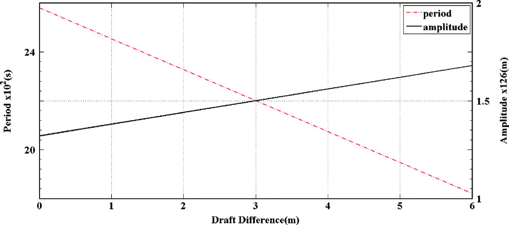
Figure 9. Period, amplitude and trim (draught difference).

Table 2. Computed and Measured Results.

(C – computed, M – measured).

5. VALIDATION OF THE SIMULATION RESULTS

In order to verify the validity of the numerical simulation models for the Capesize ships, a real time model test has been conducted for the 180,000 DWT Capesize ship with full load moored by means of a single hall anchor (port side) at a water depth of 35·6 m at Qingdao anchorage (mud bottom). The wind and current were generated by nature and recorded by electric instruments. The ship's positions, headings and time were recorded each second. The yaw motion was measured by virtue of a polarization filter. The chain tension was measured with a ring-shaped force transducer incorporated in the chain near the attachment point at the bow. This device is capable of sensing the changes of the force on the chain and transforms the signals into the actual force. The operation of this chain tension meter could have greatly contributed to the better understanding of how the chain force varied with time. Unfortunately, it failed in measuring the anchor holding force due to a technical fault. The results are given in Figures 2 to 9 and Table 2.

6. ANALYSIS OF SIMULATION AND MODEL TEST RESULTS

The comparison of the actual observations and the numerical simulations is shown in Figures 2 to 9 and Table 2. Figures 2 to 9 and Table 2 revealed that the results of simulation and practical testing at anchor are generally in agreement. The low frequency varying motions are dominant for horizontal plane modes (surge-sway-yaw), while wave frequency motions are pronounced for vertical plane modes (heave-roll-pitch). The simulation and observation results have also verified the reasonable nature of the assumptions that large size ships have negligible heave, roll and pitch motions compared with smaller size ships at anchor. However, large size ships have considerable added mass and inertia moments.

6.1. Trajectory of the motions

It is noted that the trajectory of the motions on horizontal plane appeared to be a ‘Figure 8’ shape of “∞”, but was not exactly the same each time. The noticeable shrinking on the left part of the measured trajectory is probably linked to the off-centre position of the chain (portside) compared to the previous assumption for the centreline. So a significant discrepancy can be seen between the computed and measured trajectories.

6.2. Wind Force

The period of the motions is significantly affected by the wind force. Stronger wind usually yields a shorter period but a bigger amplitude. The simulations have demonstrated that the peak period in wind force 9 m/s is about 10 minutes longer than that in wind force 17 m/s, but the maximum amplitude is about 70 m shorter.

6.3. Length of chain – length of ship ratio

The period of motions with L _c/L≈7(length of chain – length of ship ratio) is about 8 minutes longer than that of motions with L _c/L≈4 and, accordingly, the amplitude is 31 m larger. Clearly, a longer length of chain can significantly reduce the sway and produce much more holding power and lateral restoring force; however, excessive chain length would increase the swinging circle of the ship and could increase the possibility of collision with surrounding ships at anchor.

6.4. Chain Tension

The tension on the chain varies sinusoidally or, sinusoidally-like, in one cycle and reaches the maximum when the heading is in line with the chain and comes to its minimum when the transverse displacement arrives at the extremes. To prevent the ship from dragging its anchor, the anchor holding force should always be larger than the chain tension.

6.5. Current Velocity

The current can create small effects on the period and amplitude when it is in the same direction as the wind but, depending on the environmental and ship conditions, it may have a much larger influence when the directions are different.

6.6. Trim (Difference of draught forward/aft)

Trim (difference of draught forward/aft) has a significant influence on the period and amplitude of the motions (Wenxian Gu, Reference Wenxian1996). The simulations have indicated that the period will increase by about 7 minutes and the amplitude will shrink by about 46 m if a reduction of trim from 5 m to zero is made. Thus, keeping the ship's trim level or a slightly down by the head during high winds is an effective way to decrease the motions of ship at anchor.

7. CONCLUSIONS

In this paper, the motions of an anchored Capesize ship and the relationship between the period, amplitude and length of chain and environmental factors such as water depth, wind force, current, etc., are numerically simulated and the numerical results are compared with the actual observed results at Qingdao anchorage. The results have shown that:

• The numerical results are generally in conformity with the actual observed results.
• The motions of anchored vessels are highly nonlinear and need nonlinear methods for the solutions.
• The length of anchor chain is determined by the environmental conditions such as water depth, wind, current, waves, etc., and the state of the vessel as well.
• Trim has significant influence on the motions of an anchored ship; keeping the ship level or a slightly down by the head during high winds can increase the period and shorten the amplitude.
• For a given anchoring system, the limiting water depth and the environmental conditions in which a safe anchoring operation is required can be determined with the assistance of the computational results presented. The length of chain in this study is calculated on the basis of a sea bottom of mud, therefore more shackles of cable should be used if the sea bottom is composed of sand or mixed ground.

The simulated results can provide mariners with good guidance for anchoring operations, particularly for large vessels. Further research is also needed to conduct a series of scale model tests in different environmental conditions including strong wind and waves at an anchorage. A more advanced instrument to measure the anchor holding force will also be required. A future study of this nature will provide further datasets for validation of the numerical model and the level of agreement between the numerical and the observed results will determine the next step. If the level of agreement is good, the model could be extended to include motion coupling and shallow water effects, backed up by further model tests.

References

REFERENCES

Biguang, H. (1989). Analysis of ship oscillation in low frequency and prediction of ship dragging under the influence of wind and current. Journal of Dalian Maritime University, 15, 129–132.Google Scholar

Boyd, S. P., Ghaoui, L. E., Feron, E. and Balakrishnan, V. (1994). Linear Matrix Inequalities in Systems and Control Theory, Philadelphia, PA: SIAM.CrossRef Google Scholar

Chakrabarti, S. (2001). Empirical calculation of roll damping for ships and barges. Ocean Engineering, 28, 915–932.CrossRef Google Scholar

Fossen, T. I. (1994). Guidance and Control of Ocean Vehicles, Wiley, New York.Google Scholar

Fossen, T. I. and Grovlen, A. (1998). Nonlinear output feedback control of dynamically positioned ships using vectorial observer backstepping. IEEE Trans. on Control Systems Technology, 6–1, 121–128Google Scholar

Godhavn, J. M., Fossen, T. I. and Berge, S. P. (1998). Nonlinear and adaptive backstepping designs for tracking control of ships. Int. J. Adaptive Control and Signal Processing, 12-8, 649–670.Google Scholar

Heshu, L, Weiqing, J. and Baochun, Y. (1995). Mathematical model of predicting ship dragging. Navigation of China, 1, 128–130.Google Scholar

Jaroslaw, A. (2003). Anchor forces in ship manoeuvring mathematical model. Annual of Navigation, 6, 5–17.Google Scholar

Jiachang, Y., Zuochang, Y. and Yuyang, . (2005). Early warning system of anchor dragging. Journal of Dalian Maritime University, 31, 29–31.Google Scholar

Kim, M. H., Ran, Z. and Zheng, W. (2001). Hull/mooring coupled dynamic analysis of a truss spar in time domain. Int. Journal of Offshore and Polar Engineering, Vol. 11, No. 1, 42–54.Google Scholar

Klaka, K., Krokstad, J. and Renilson, M. R. (2003). Prediction and measurement of the roll motion of a sailing yacht at zero forward speed. Experimental Thermal and Fluid Science, 27, 611–617.Google Scholar

Nesterov, Y. and Nemirovski, A. (1994). Interior Point Polynomial Methods in Convex Programming: Theory and Application. Philadelphia. SIAM Books.Google Scholar

Sariöz, K. and Narli, E. (2003). Assessment of manoeuvring performance of large tankers in restricted waterways: a realtime simulation approach. Ocean Engineering, 30, 1535–1551.Google Scholar

Wenjerchang, Guojang Chen and Yilin, Yeh. (2002). Fuzzy control of dynamic positioning systems for ships. Journal of Marine Science and Technology, 10-1, 47–53.Google Scholar