


1. Introduction
The study of hydrodynamic behaviour allows us to deal with infinite-dimensional models that appear in statistical mechanics and engineering. It is an important tool in different areas of natural, social, and physical sciences (such as traffic flow, pedestrian flow, the components of a cell, expansion of epidemics or fire, etc.), where the techniques do not seek to measure the individual activity of the particle (a pedestrian, a neuron, a car, etc), but the effect resulting from the interaction of large sets of particles. Thus, mathematical modelling requires a macroscopic description (macroscopic equation of the system) derived from many particles interacting (microscopic systems), which is a typical setting of study on hydrodynamic limits of stochastic particle systems.
Mathematically, the components are modelled as particles confined in a discrete geometry. A major question is how to perform the limit from the discrete to the continuum in such a way that the discretization of the system gives the correct description of the continuum. The issue is to characterize the distribution in later times, given that we started with a measure of local equilibrium. That is, considering an initial density profile
 $\rho_0$
, is there a function that represents the density profile in future times? The answer is given by the temporal and spatial scales that are chosen for this problem. Through this re-escalation, it is possible to have a microscopic view of the position of the particles in the system, and the time is accelerated so that the movement in the system is observed. Kipnis and Landim [Reference Kipnis and Landim9] treated the limit of several particle systems and can be seen as the main reference on the subject.
$\rho_0$
, is there a function that represents the density profile in future times? The answer is given by the temporal and spatial scales that are chosen for this problem. Through this re-escalation, it is possible to have a microscopic view of the position of the particles in the system, and the time is accelerated so that the movement in the system is observed. Kipnis and Landim [Reference Kipnis and Landim9] treated the limit of several particle systems and can be seen as the main reference on the subject.
On the other hand, another important subject in statistical physics is the characterization of the hydrodynamic behaviour of interacting particle systems in random environments. In recent years several approaches have been developed in order to study this problem. We point out some results on the subject, most related to the symmetric simple exclusion process, as they have in common the relation between the exponential clock and the bonds, having the Bernoulli product measure as an invariant measure. Faggionato et al. [Reference Faggionato, Jara and Landim1] considered a system of particles performing nearest-neighbour random walks on the lattice
 $\mathbb{Z}$
under hard-core interaction. In this case, the hydrodynamic equation results in the weak heat equation. Jara [Reference Jara6] established general sufficient conditions for the hydrodynamic limit of the exclusion process in an inhomogeneous environment. These works inspired developments in the context of particle systems in [Reference Franco, Gonçalves and Neumann2] and [Reference Franco, Neumann and Valle3]. Franco et al. [Reference Franco, Neumann and Valle3] considered slow bonds with a smaller clock parameter, which makes the passage of particles across the corresponding bond more difficult. The authors obtained a d-dimensional result for a model in which the slow bonds are close to a smooth surface. Along the same lines, Franco et al. [Reference Franco, Gonçalves and Neumann2] considered k fixed slower clocks in a discrete torus with N sites. The slower clock has a parameter given by
$\mathbb{Z}$
under hard-core interaction. In this case, the hydrodynamic equation results in the weak heat equation. Jara [Reference Jara6] established general sufficient conditions for the hydrodynamic limit of the exclusion process in an inhomogeneous environment. These works inspired developments in the context of particle systems in [Reference Franco, Gonçalves and Neumann2] and [Reference Franco, Neumann and Valle3]. Franco et al. [Reference Franco, Neumann and Valle3] considered slow bonds with a smaller clock parameter, which makes the passage of particles across the corresponding bond more difficult. The authors obtained a d-dimensional result for a model in which the slow bonds are close to a smooth surface. Along the same lines, Franco et al. [Reference Franco, Gonçalves and Neumann2] considered k fixed slower clocks in a discrete torus with N sites. The slower clock has a parameter given by
 ${N}^{{-}\beta}$
, with
${N}^{{-}\beta}$
, with
 $\beta \in [0,\infty]$
. According to the value of
$\beta \in [0,\infty]$
. According to the value of
 $\beta$
, three different limits for the time trajectory of the spatial density of particles were obtained. If
$\beta$
, three different limits for the time trajectory of the spatial density of particles were obtained. If
 $\beta \in [0,1),$
the limit is given by the weak solution of the periodic heat equation, so the slow bond is not slow enough to originate any change in the continuum. If
$\beta \in [0,1),$
the limit is given by the weak solution of the periodic heat equation, so the slow bond is not slow enough to originate any change in the continuum. If
 $\beta=1$
, the limit is given by the weak solution of the heat equation with some Robin’s boundary condition, and Franco et al. [Reference Franco, Gonçalves and Neumann2] presented a quick proof of the particles’ density time evolution for this process. If
$\beta=1$
, the limit is given by the weak solution of the heat equation with some Robin’s boundary condition, and Franco et al. [Reference Franco, Gonçalves and Neumann2] presented a quick proof of the particles’ density time evolution for this process. If
 $\beta \in (1,\infty]$
, the limit is given by the weak solution of the heat equation with Neumann’s boundary condition. On the contrary, in [Reference Seppäläinen13] the totally asymmetric simple exclusion process is considered to have a single bond with a smaller clock parameter. In this case, the slow bond parameter does not need to be rescaled in order to have a macroscopic influence.
$\beta \in (1,\infty]$
, the limit is given by the weak solution of the heat equation with Neumann’s boundary condition. On the contrary, in [Reference Seppäläinen13] the totally asymmetric simple exclusion process is considered to have a single bond with a smaller clock parameter. In this case, the slow bond parameter does not need to be rescaled in order to have a macroscopic influence.
As described above, a relevant problem is to consider particle systems with slow bonds and to analyze the macroscopic effect on the hydrodynamic profiles. As a particular case of [Reference Faggionato, Jara and Landim1] and [Reference Franco, Gonçalves and Neumann2], in this paper we address the complete characterization of the hydrodynamic limit scenario for the exclusion process in a discrete torus, with N sites, and with random slow bonds
 $\lambda/N$
(
$\lambda/N$
(
 $ \lambda \in ( 0,1]) $
defined in terms of a random environment given by a homogeneous Poisson process on the real line. As [Reference Franco, Gonçalves and Neumann2] includes a simple quenched proof when the slower clock has a parameter given by
$ \lambda \in ( 0,1]) $
defined in terms of a random environment given by a homogeneous Poisson process on the real line. As [Reference Franco, Gonçalves and Neumann2] includes a simple quenched proof when the slower clock has a parameter given by
 $1/N$
, for the sake of completeness, we show here a detailed proof. For the other slow bonds of our problem, Franco [Reference Franco, Gonçalves and Neumann2] showed a complete proof of the hydrodynamic quenched limit, so we use those results directly.
$1/N$
, for the sake of completeness, we show here a detailed proof. For the other slow bonds of our problem, Franco [Reference Franco, Gonçalves and Neumann2] showed a complete proof of the hydrodynamic quenched limit, so we use those results directly.
We can think that the process describes the transport of particles in a one-dimensional medium with strong random barriers established in the marks of a homogeneous Poisson process on
 $\mathbb{R}$
with intensity
$\mathbb{R}$
with intensity
 $\lambda$
. Such slow bonds do not only slow down the passage of particles across it, but they also have a macroscopic impact since it disturbs the hydrodynamic profile. We study the hydrodynamic limit of the exclusion process under diffusive rescaling, both in an annealed form and in a quenched form.
$\lambda$
. Such slow bonds do not only slow down the passage of particles across it, but they also have a macroscopic impact since it disturbs the hydrodynamic profile. We study the hydrodynamic limit of the exclusion process under diffusive rescaling, both in an annealed form and in a quenched form.
In this sense, we consider the nearest-neighbour simple exclusion process on the one-dimensional discrete torus
 $\mathbb{T}_N=\mathbb{Z}/N\mathbb{Z}$
, with random rates
$\mathbb{T}_N=\mathbb{Z}/N\mathbb{Z}$
, with random rates
 $c_N=\{c_{x,N}\colon x \in \mathbb{T}_N\}$
defined in terms of a homogeneous Poisson process on
$c_N=\{c_{x,N}\colon x \in \mathbb{T}_N\}$
defined in terms of a homogeneous Poisson process on
 $\mathbb{R}$
with intensity
$\mathbb{R}$
with intensity
 $\lambda$
. Given a realization of the Poisson process, the jump rate along the edge
$\lambda$
. Given a realization of the Poisson process, the jump rate along the edge
 $\{x,x+1\}$
is 1 (
$\{x,x+1\}$
is 1 (
 $c_{x,N}=1$
) if there is not any Poisson mark in
$c_{x,N}=1$
) if there is not any Poisson mark in
 $ (x,x+1) $
; otherwise, it is
$ (x,x+1) $
; otherwise, it is
 $\lambda/N,\, \lambda \in ( 0,1 ]$
.
$\lambda/N,\, \lambda \in ( 0,1 ]$
.
Obtaining the density profile in future times, we study the behaviour of a tagged particle given an initial configuration based on clusters of size j. A configuration based on clusters of size j assigns very high probability to the interval
 $[ -j , j] $
, with j a positive integer, and a probability very close to 0 outside this interval. The tagged particle is the particle that is positioned in the center of the cluster. The stochastic clusters are defined in such a way the initial profile has a fourth bounded derivative. We focus on the ability of the tagged particle motion and, in particular, the first displacement time of the tagged particle.
$[ -j , j] $
, with j a positive integer, and a probability very close to 0 outside this interval. The tagged particle is the particle that is positioned in the center of the cluster. The stochastic clusters are defined in such a way the initial profile has a fourth bounded derivative. We focus on the ability of the tagged particle motion and, in particular, the first displacement time of the tagged particle.
The asymptotic behaviour of a tagged particle is one of the central problems in the theory of particle systems and there are still many unresolved issues. Kipnis and Varadhan [Reference Kipnis and Varadhan10] gave the first important result related to the position of the particle. The authors deduced an equilibrium central limit theorem for a symmetric simple exclusion process. The method relies on a central limit theorem for additive functionals of Markov processes and uses time reversibility and translation invariance. This result was extended in [Reference Varadhan16] for mean-zero asymmetric exclusion processes and in [Reference Sethuraman, Varadhan and Yau14] for dimension
 $d \geq 3$
. Rezakhanlou [Reference Rezakhanlou12] proved a propagation of the chaos result, which states that the average behaviour of tagged particles is described by a diffusion process. In the sequence, Jara and Landim [Reference Jara and Landim7] proved the first nonequilibrium central limit theorem for the position of a tagged particle in the one-dimensional nearest-neighbour symmetric simple exclusion process under diffusive scaling starting from a Bernoulli product measure associated to a smooth profile. These studies supported the results in [Reference Gonçalves4], where the authors proved a central limit theorem for the position of a tagged particle in the one-dimensional asymmetric simple exclusion process in the hyperbolic scaling. The authors also proved that the position of the tagged particle at time t depends on the initial configuration.
$d \geq 3$
. Rezakhanlou [Reference Rezakhanlou12] proved a propagation of the chaos result, which states that the average behaviour of tagged particles is described by a diffusion process. In the sequence, Jara and Landim [Reference Jara and Landim7] proved the first nonequilibrium central limit theorem for the position of a tagged particle in the one-dimensional nearest-neighbour symmetric simple exclusion process under diffusive scaling starting from a Bernoulli product measure associated to a smooth profile. These studies supported the results in [Reference Gonçalves4], where the authors proved a central limit theorem for the position of a tagged particle in the one-dimensional asymmetric simple exclusion process in the hyperbolic scaling. The authors also proved that the position of the tagged particle at time t depends on the initial configuration.
Jara and Landim [Reference Jara and Landim8] extended the approach of [Reference Kipnis and Varadhan10] to interacting particle systems whose generators satisfy a sector condition or, more generally, graded sector conditions. The authors studied a quenched nonequilibrium central limit theorem for the position of a tagged particle in the exclusion process, where the bonds disorder
 $\{\psi_x \colon x \in \mathbb{Z}\}$
are independent and identically distributed (i.i.d.) random variables bounded above and below by strictly positive finite constants. It was proved that the position of the tagged particle converges under diffusive scaling to a Gaussian process if the other particles are initially distributed according to a Bernoulli product measure associated to a smooth initial profile. The work of [Reference Jara5] extended [Reference Kipnis and Landim9] for the case of an exclusion process with long jumps. This is a simple exclusion process with transition rate
$\{\psi_x \colon x \in \mathbb{Z}\}$
are independent and identically distributed (i.i.d.) random variables bounded above and below by strictly positive finite constants. It was proved that the position of the tagged particle converges under diffusive scaling to a Gaussian process if the other particles are initially distributed according to a Bernoulli product measure associated to a smooth initial profile. The work of [Reference Jara5] extended [Reference Kipnis and Landim9] for the case of an exclusion process with long jumps. This is a simple exclusion process with transition rate
 $p(x, y) = \smash{|y - x|^{(-d-\alpha)},\, \alpha
\in (0, 2)}$
. The authors obtained a nonequilibrium invariance principle for the position of a tagged particle. The limiting process is a time-inhomogeneous process of independent increments, driven by a solution u(t, x) of the fractional heat equation
$p(x, y) = \smash{|y - x|^{(-d-\alpha)},\, \alpha
\in (0, 2)}$
. The authors obtained a nonequilibrium invariance principle for the position of a tagged particle. The limiting process is a time-inhomogeneous process of independent increments, driven by a solution u(t, x) of the fractional heat equation
 $\partial_tu =
\Lambda^{\alpha/2}$
, where
$\partial_tu =
\Lambda^{\alpha/2}$
, where
 $\Lambda^{\alpha/2}$
is the fractional Laplacian. In the equilibrium case, the limiting process is a symmetric,
$\Lambda^{\alpha/2}$
is the fractional Laplacian. In the equilibrium case, the limiting process is a symmetric,
 $\alpha$
-stable Lévy process.
$\alpha$
-stable Lévy process.
The main reference for the most advanced theories on the martingale approach to central limit theorems is [Reference Jara5]. In this reference the techniques that allow us to deal with the problem of the central limit theorem of interacting particle systems, homogenization in random environments, diffusion in turbulent flows, etc, are developed.
For
 $\lambda \in ( 0,1),$
by [Reference Franco, Gonçalves and Neumann2], the density profile of the process proposed in this work with the initial Bernoulli product measure associated to an initial profile
$\lambda \in ( 0,1),$
by [Reference Franco, Gonçalves and Neumann2], the density profile of the process proposed in this work with the initial Bernoulli product measure associated to an initial profile
 $\rho_0\colon \mathbb{R} \rightarrow
[0,1]$
, evolves as the solution of
$\rho_0\colon \mathbb{R} \rightarrow
[0,1]$
, evolves as the solution of
 \begin{gather}
\partial_t\rho = \Delta\rho \text{ in } (\gamma_j,\gamma_{j+1}),\tag{1.1a}\label{eqn1}\end{gather}
\begin{gather}
\partial_t\rho = \Delta\rho \text{ in } (\gamma_j,\gamma_{j+1}),\tag{1.1a}\label{eqn1}\end{gather}
 \begin{gather}
\partial_x\rho(t,\gamma_j {+}) = \partial_x\rho(t,\gamma_j {-})=0,\tag{1.1b}\label{eqn2}\end{gather}
\begin{gather}
\partial_x\rho(t,\gamma_j {+}) = \partial_x\rho(t,\gamma_j {-})=0,\tag{1.1b}\label{eqn2}\end{gather}
 \begin{gather}
\rho(0,\cdot) = \rho^{ j}_0({\cdot}),\tag{1.1c}
\label{eqn3}\end{gather}
\begin{gather}
\rho(0,\cdot) = \rho^{ j}_0({\cdot}),\tag{1.1c}
\label{eqn3}\end{gather}
where
 $\Delta \rho$
is the Laplacian of
$\Delta \rho$
is the Laplacian of
 $\rho$
and
$\rho$
and
 $\gamma_{k}$
represent the sequence of Poisson marks on
$\gamma_{k}$
represent the sequence of Poisson marks on
 $ \mathbb{R} $
. Here, the subindex k means that there is a Poisson mark in
$ \mathbb{R} $
. Here, the subindex k means that there is a Poisson mark in
 $ k \in \mathbb{R} $
and
$ k \in \mathbb{R} $
and
 $\gamma_{l}$
is the first Poisson mark after
$\gamma_{l}$
is the first Poisson mark after
 $\gamma_{k}$
.
$\gamma_{k}$
.
On the other hand, in some sense, the technical steps to describe the hydrodynamic behaviour of the process proposed when
 $\lambda=1$
follow the techniques developed in [Reference Faggionato, Jara and Landim1]. We prove that the density profile of this process evolves as the solution of the bounded diffusion random equation.
$\lambda=1$
follow the techniques developed in [Reference Faggionato, Jara and Landim1]. We prove that the density profile of this process evolves as the solution of the bounded diffusion random equation.
 \begin{equation}
\begin{gathered}
\partial_t\rho = \Delta\rho \text{ in } (\gamma_k,\gamma_{l}),
\\
\partial_x\rho(t,\gamma_k {+}) = \partial_x\rho(t,\gamma_k {-}),
\\
\partial_x\rho(t, \gamma_k{+}) = \lambda [\rho(t,\gamma_k {-}) -
\rho(t,\gamma_k {+}) ].
\end{gathered}
\end{equation}
\begin{equation}
\begin{gathered}
\partial_t\rho = \Delta\rho \text{ in } (\gamma_k,\gamma_{l}),
\\
\partial_x\rho(t,\gamma_k {+}) = \partial_x\rho(t,\gamma_k {-}),
\\
\partial_x\rho(t, \gamma_k{+}) = \lambda [\rho(t,\gamma_k {-}) -
\rho(t,\gamma_k {+}) ].
\end{gathered}
\end{equation}
Given the density profile for the process when
 $\lambda \in ( 0,1] $
and the initial configuration based on clusters of size
$\lambda \in ( 0,1] $
and the initial configuration based on clusters of size
 $j \in \mathbb{Z}$
, the characterization of the first displacement time of a tagged particle in a stochastic cluster (the core of the cluster) is stated. To the best of the authors’ knowledge, no similar phenomena has been exploited in the field of the hydrodynamic limit of interacting particle systems, so it is the main contribution of this article.
$j \in \mathbb{Z}$
, the characterization of the first displacement time of a tagged particle in a stochastic cluster (the core of the cluster) is stated. To the best of the authors’ knowledge, no similar phenomena has been exploited in the field of the hydrodynamic limit of interacting particle systems, so it is the main contribution of this article.
The strategy of the proof consists in considering an approximation in discrete time of the solution of the hydrodynamic bounded diffusion equation
 $\rho_J,$
which describes the process stated above. Using this approach and the Cauchy–Peano existence theorem of differential equations, we prove that the solution of the discrete linear equation approximates
$\rho_J,$
which describes the process stated above. Using this approach and the Cauchy–Peano existence theorem of differential equations, we prove that the solution of the discrete linear equation approximates
 $\rho_J$
by
$\rho_J$
by
 $N^{{-}2}$
.
$N^{{-}2}$
.
In order to achieve our goal, the main difficulties appear in establishing the number of times the origin became vacant in a fixed interval. We overcome this difficulty by defining a Poisson process
 $\smash{N_t^{\{x,y\}}}$
for
$\smash{N_t^{\{x,y\}}}$
for
 $x,y \in \mathbb{T}_N$
by
$x,y \in \mathbb{T}_N$
by
 \begin{equation}
N_t^{\{x,y\}}=\sum_{k\geq 1}\textbf{1}_{\{\tau_k^{(x,y)}\leq t\}}
\end{equation}
\begin{equation}
N_t^{\{x,y\}}=\sum_{k\geq 1}\textbf{1}_{\{\tau_k^{(x,y)}\leq t\}}
\end{equation}
for
 $t>0$
and
$t>0$
and
 $\smash{N_0^{\{x,y\}}=0}$
, where
$\smash{N_0^{\{x,y\}}=0}$
, where
 $\smash{\{\tau_k^{(x,y)}\colon k \geq\}}$
are independent Poisson processes at the edges (x,y). Here
$\smash{\{\tau_k^{(x,y)}\colon k \geq\}}$
are independent Poisson processes at the edges (x,y). Here
 $\smash{\{\tau_k^{(x,y)}\}}$
can be interpreted as random instants of times in which the particles try to move from x to y.
$\smash{\{\tau_k^{(x,y)}\}}$
can be interpreted as random instants of times in which the particles try to move from x to y.
We define the number of times the origin becomes vacant, in a fixed interval, as a function of the process
 $\smash{N_t^{\{x,y\}}}$
and obtain upper and lower bounds for the distribution of the escape time of the particle at the origin.
$\smash{N_t^{\{x,y\}}}$
and obtain upper and lower bounds for the distribution of the escape time of the particle at the origin.
The structure of the article is as follows. In Section 2 we introduce notation, give precise definitions of the simple exclusion process with slow random bonds and of the stochastic cluster objects of our study, and state the main results. In Section 3 we characterize the hydrodynamic behaviour of the process over large space and time scales, and we prove that the solution of the partial differential equation that describes the macroscopic evolution of the system is unique. In Section 4 we state an estimate on the difference of the solution of the hydrodynamic equation and the solution of a discretized version of the hydrodynamic equation. Finally, in Section 5 we characterize the time of first displacement of the stochastic cluster core in the simple exclusion process with random slow bonds.
2. Notation, definitions, and results
Henceforth we will use the following notation for a nonempty set A: let C(A) denote the space of continuous real functions on A,
 $C_b(A) $
denote the space of bounded continuous real functions on A,
$C_b(A) $
denote the space of bounded continuous real functions on A,
 $C_c(A) $
denote the space of continuous real functions with compact support, and
$C_c(A) $
denote the space of continuous real functions with compact support, and
 $C_0(A) $
denote the real bounded continuous functions such that, for any
$C_0(A) $
denote the real bounded continuous functions such that, for any
 $\epsilon >0,$
the function has modulus smaller than
$\epsilon >0,$
the function has modulus smaller than
 $\epsilon$
outside a suitable bounded subset
$\epsilon$
outside a suitable bounded subset
 $F \subset A$
(functions that vanish at
$F \subset A$
(functions that vanish at
 $\infty$
).
$\infty$
).
Consider the exclusion process on the state space
 $\{0,1\}^\mathbb{Z}$
with random rates
$\{0,1\}^\mathbb{Z}$
with random rates
 $c=\{c_x\colon x \in \mathbb{Z}\}$
defined in terms of a homogeneous Poisson process on
$c=\{c_x\colon x \in \mathbb{Z}\}$
defined in terms of a homogeneous Poisson process on
 $\mathbb{R}$
with intensity
$\mathbb{R}$
with intensity
 $\lambda$
. Here
$\lambda$
. Here
 $\{\gamma_{k}\colon k \in \mathbb{Z}\}$
are the successive marks of the Poisson process. Given a realization of the Poisson process,
$\{\gamma_{k}\colon k \in \mathbb{Z}\}$
are the successive marks of the Poisson process. Given a realization of the Poisson process,
 $c_x=\lambda$
if there is a Poisson mark in the interval
$c_x=\lambda$
if there is a Poisson mark in the interval
 $ (x,x+1) $
and
$ (x,x+1) $
and
 $c_x=1$
otherwise. Denote by
$c_x=1$
otherwise. Denote by
 $\dot{\eta}$
the configurations of
$\dot{\eta}$
the configurations of
 $\{0,1\}^{\mathbb{Z}}$
so that
$\{0,1\}^{\mathbb{Z}}$
so that
 $\dot{\eta}(x)=1$
if site x is not vacant and
$\dot{\eta}(x)=1$
if site x is not vacant and
 $\dot{\eta}(x)=0$
otherwise. At rate
$\dot{\eta}(x)=0$
otherwise. At rate
 $c_x$
the variables
$c_x$
the variables
 $\dot{\eta}(x) $
and
$\dot{\eta}(x) $
and
 $\dot{\eta}(x+1) $
are exchanged.
$\dot{\eta}(x+1) $
are exchanged.
The generator
 $\dot{L}$
of this Markov process can be written as
$\dot{L}$
of this Markov process can be written as
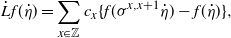 \begin{equation}
\dot{L}f(\dot{\eta})=\sum_{x \in \mathbb{Z}}c_x\{ f(\sigma^{x,x+1}
\dot{\eta})-f(\dot{\eta})\},
\label{eqn4}
\end{equation}
\begin{equation}
\dot{L}f(\dot{\eta})=\sum_{x \in \mathbb{Z}}c_x\{ f(\sigma^{x,x+1}
\dot{\eta})-f(\dot{\eta})\},
\label{eqn4}
\end{equation}
where f is a cylindrical function and
 $\sigma^{x,x+1}\dot{\eta}$
is the configuration obtained from
$\sigma^{x,x+1}\dot{\eta}$
is the configuration obtained from
 $\dot{\eta}$
by exchanging the variables
$\dot{\eta}$
by exchanging the variables
 $\dot{\eta}(x), \dot{\eta}(x+1) $
:
$\dot{\eta}(x), \dot{\eta}(x+1) $
:
 \begin{equation}
\sigma^{x,x+1}\dot{\eta}( y)=
\begin{cases}
\dot{\eta}(x+1) & \textrm{if} \; y=x,
\\
\dot{\eta}(x) & \textrm{if}\; y=x+1,
\\
\dot{\eta}( y) & \textrm{otherwise.}
\end{cases}
\end{equation}
\begin{equation}
\sigma^{x,x+1}\dot{\eta}( y)=
\begin{cases}
\dot{\eta}(x+1) & \textrm{if} \; y=x,
\\
\dot{\eta}(x) & \textrm{if}\; y=x+1,
\\
\dot{\eta}( y) & \textrm{otherwise.}
\end{cases}
\end{equation}
In order to obtain the annealed result of this exclusion process, we consider the nearest-neighbour simple exclusion process on the one-dimensional discrete torus
 $\mathbb{T}_N= \mathbb{Z}/N\mathbb{Z}, $
with N sites and with random rates
$\mathbb{T}_N= \mathbb{Z}/N\mathbb{Z}, $
with N sites and with random rates
 $c_N=\{c_{x,N}\colon x \in \mathbb{T}_N\}$
defined in terms of the Poisson process on
$c_N=\{c_{x,N}\colon x \in \mathbb{T}_N\}$
defined in terms of the Poisson process on
 $\mathbb{R}$
with intensity
$\mathbb{R}$
with intensity
 $\lambda$
. Given a realization of the Poisson process, the jump rate along the edge
$\lambda$
. Given a realization of the Poisson process, the jump rate along the edge
 $\{x,x+1\}$
is 1 (
$\{x,x+1\}$
is 1 (
 $c_{x,N}=1$
) if there is not a Poisson mark in the interval
$c_{x,N}=1$
) if there is not a Poisson mark in the interval
 $ (x,x+1) $
; otherwise, it is
$ (x,x+1) $
; otherwise, it is
 $\lambda/N, \lambda \in ( 0,1] $
.
$\lambda/N, \lambda \in ( 0,1] $
.
We consider a particular case of [Reference Faggionato, Jara and Landim1] to get a random number of slow bonds. Note that the rates
 $c_N=\{c_{x,N}\colon x \in
\mathbb{T}_N\}$
have the same distribution as
$c_N=\{c_{x,N}\colon x \in
\mathbb{T}_N\}$
have the same distribution as
 $\{c_x\colon x \in \mathbb{Z}\}$
for each
$\{c_x\colon x \in \mathbb{Z}\}$
for each
 $N \geq 1$
. Then we use the hydrodynamic profiles for this model to obtain the first displacement time of a tagged particle when
$N \geq 1$
. Then we use the hydrodynamic profiles for this model to obtain the first displacement time of a tagged particle when
 $\lambda \in
( 0,1] $
.
$\lambda \in
( 0,1] $
.
Denote by
 $\eta$
the configurations of
$\eta$
the configurations of
 $\smash{\{0,1\}^{\mathbb{T}_N}}$
, consisting of a vector with n components, each one taking the value 0 or 1, so that
$\smash{\{0,1\}^{\mathbb{T}_N}}$
, consisting of a vector with n components, each one taking the value 0 or 1, so that
 $\eta(x)=1$
if site x is not vacant and
$\eta(x)=1$
if site x is not vacant and
 $\eta(x)=0$
otherwise. At rate
$\eta(x)=0$
otherwise. At rate
 $c_{x,N}$
the variables
$c_{x,N}$
the variables
 $\eta(x) $
and
$\eta(x) $
and
 $\eta(x+1) $
are exchanged.
$\eta(x+1) $
are exchanged.
The generator L of this Markov process can be written as
 \begin{equation}
Lf(\eta)=\sum_{x \in \mathbb{T}_N}c_{x,N}\{ f(\sigma^{x,x+1}\eta)-f(\eta)\},
\end{equation}
\begin{equation}
Lf(\eta)=\sum_{x \in \mathbb{T}_N}c_{x,N}\{ f(\sigma^{x,x+1}\eta)-f(\eta)\},
\end{equation}
where f is a local function and
 $\sigma^{x,x+1}\eta$
is the configuration obtained from
$\sigma^{x,x+1}\eta$
is the configuration obtained from
 $\eta$
by exchanging the variables
$\eta$
by exchanging the variables
 $\eta(x) $
,
$\eta(x) $
,
 $\eta(x+1) $
:
$\eta(x+1) $
:
 \begin{equation}
\sigma^{x,x+1}\eta( y)=
\begin{cases}
\eta(x+1) & \textrm{if} \; y=x,
\\
\eta(x) & \textrm{if}\; y=x+1,
\\
\eta( y) & \textrm{otherwise.}
\end{cases}
\end{equation}
\begin{equation}
\sigma^{x,x+1}\eta( y)=
\begin{cases}
\eta(x+1) & \textrm{if} \; y=x,
\\
\eta(x) & \textrm{if}\; y=x+1,
\\
\eta( y) & \textrm{otherwise.}
\end{cases}
\end{equation}

Figure 1. Simulation of W for different values of
 $\lambda$
and fixed N (
$\lambda$
and fixed N (
 $N=10$
).
$N=10$
).
The array
 $\{c_{y,N}\colon y \in \mathbb{T}_N\}$
can be constructed as
$\{c_{y,N}\colon y \in \mathbb{T}_N\}$
can be constructed as
 \begin{equation}
c_{y,N}=\frac{1}{N\{W({( y+1)}/{N})-W({y}/{N})\}},
\label{eqn5}
\end{equation}
\begin{equation}
c_{y,N}=\frac{1}{N\{W({( y+1)}/{N})-W({y}/{N})\}},
\label{eqn5}
\end{equation}
where
 $W\colon \mathbb{R} \rightarrow \mathbb{R}$
is defined as
$W\colon \mathbb{R} \rightarrow \mathbb{R}$
is defined as
 \[
W(z)=z +\sigma(z) \bigg(\frac{1}{\lambda}-\frac{1}{N}\bigg)
\sum_{j=0}^{\infty}\textbf{1}_{\{\gamma_{j}\in [0,zN]\}},
\]
\[
W(z)=z +\sigma(z) \bigg(\frac{1}{\lambda}-\frac{1}{N}\bigg)
\sum_{j=0}^{\infty}\textbf{1}_{\{\gamma_{j}\in [0,zN]\}},
\]
where
 $\sigma(z)=1$
if
$\sigma(z)=1$
if
 $z \geq 0, \sigma(z)=-1$
if
$z \geq 0, \sigma(z)=-1$
if
 $z \lt 0$
, so that we consider a particular case of W to get a random number of slow bonds.
$z \lt 0$
, so that we consider a particular case of W to get a random number of slow bonds.
Moreover, fix
 $N \geq 1, x \in \mathbb{T}_N,$
and a realization of W. Consider the random walk
$N \geq 1, x \in \mathbb{T}_N,$
and a realization of W. Consider the random walk
 $X_N(t,x) $
defined in
$X_N(t,x) $
defined in
 $\mathbb{T}_N$
starting at x which goes from x to
$\mathbb{T}_N$
starting at x which goes from x to
 $x+1$
and from
$x+1$
and from
 $x+1$
to x with rate
$x+1$
to x with rate
 $N^2$
if there is no Poisson mark; otherwise, the rate is
$N^2$
if there is no Poisson mark; otherwise, the rate is
 $\lambda N$
. The generator for this process, considering f cylindrical, can be written as
$\lambda N$
. The generator for this process, considering f cylindrical, can be written as
 \begin{equation}
(\mathbb{L}_N f)\bigg(\frac{x}{N}\bigg)=N^2c_{x,N}\{ f(x+1)-f(x)\}+
N^2c_{x-1,N}\{ f(x-1)-f(x)\}.
\label{eqn6}
\end{equation}
\begin{equation}
(\mathbb{L}_N f)\bigg(\frac{x}{N}\bigg)=N^2c_{x,N}\{ f(x+1)-f(x)\}+
N^2c_{x-1,N}\{ f(x-1)-f(x)\}.
\label{eqn6}
\end{equation}
In Figure 1 we show the simulation of W for different values of
 $\lambda$
and fixed N (
$\lambda$
and fixed N (
 $N=10$
). The triangles represent the Poisson marks on
$N=10$
). The triangles represent the Poisson marks on
 $ \mathbb{R}$
. The utility of constructing the array
$ \mathbb{R}$
. The utility of constructing the array
 $c_{y,N}$
as a function of W will be clear in Subsection 2.2, where it is established that the asymptotic behaviour of the random walk
$c_{y,N}$
as a function of W will be clear in Subsection 2.2, where it is established that the asymptotic behaviour of the random walk
 $X_N(t,x) $
can be written as a function of the jump function W.
$X_N(t,x) $
can be written as a function of the jump function W.
2.1. Results
As outlined in the introduction, as a particular case, [Reference Franco, Gonçalves and Neumann2] presents a quick proof of the particles’ density time evolution in a predetermined environment when
 $\lambda=1$
, so, for the sake of completeness, we present here its complete characterization. In addition, the annealed hydrodynamic limit of the exclusion process when
$\lambda=1$
, so, for the sake of completeness, we present here its complete characterization. In addition, the annealed hydrodynamic limit of the exclusion process when
 $\lambda
\in (0,1]$
is obtained.
$\lambda
\in (0,1]$
is obtained.
2.1.1. Hydrodynamic limit
Proposition 2.1. (Quenched result.) For
 $\lambda=1$
and
$\lambda=1$
and
 $x \in \mathbb{Z} $
, let
$x \in \mathbb{Z} $
, let
 $\rho_0\colon \mathbb{R} \rightarrow
[0,1]$
be a continuous bounded profile that vanishes at
$\rho_0\colon \mathbb{R} \rightarrow
[0,1]$
be a continuous bounded profile that vanishes at
 $\infty$
and consider a sequence
$\infty$
and consider a sequence
 $\mu^N$
of Bernoulli measures such that
$\mu^N$
of Bernoulli measures such that
 \[
\mu^N\{\eta;\ \eta (x)=1\}=\rho_0\bigg(\frac{x}{N}\bigg).
\]
\[
\mu^N\{\eta;\ \eta (x)=1\}=\rho_0\bigg(\frac{x}{N}\bigg).
\]
Then, for all
 $t>0$
, the sequence of empirical measures
$t>0$
, the sequence of empirical measures
 \begin{equation}
\pi_t^N({\rm d} u)=\frac{1}{N}\sum_{x }\eta_t(x)\delta_{x/N}({\rm d} u)
\end{equation}
\begin{equation}
\pi_t^N({\rm d} u)=\frac{1}{N}\sum_{x }\eta_t(x)\delta_{x/N}({\rm d} u)
\end{equation}
converge in probability to the measure
 $\pi_t({\rm d} u)=\rho(t,u){\rm d} u$
whose density function
$\pi_t({\rm d} u)=\rho(t,u){\rm d} u$
whose density function
 $\rho$
is the solution of
$\rho$
is the solution of
 \begin{gather}
\partial_t\rho = \Delta\rho \textrm{ in the intervals } (\gamma_j,
\gamma_{j+1}),\label{eqn7}\end{gather}
\begin{gather}
\partial_t\rho = \Delta\rho \textrm{ in the intervals } (\gamma_j,
\gamma_{j+1}),\label{eqn7}\end{gather}
 \begin{gather}
\partial_x\rho(t,\gamma_j {+}) = \partial_x\rho(t,\gamma_j {-}),\label{eqn8}\end{gather}
\begin{gather}
\partial_x\rho(t,\gamma_j {+}) = \partial_x\rho(t,\gamma_j {-}),\label{eqn8}\end{gather}
 \begin{gather}
\partial_x\rho(t, \gamma_j{+}) = \lambda [\rho(t,\gamma_j {+}) -
\rho(t,\gamma_j {-}) ],
\label{eqn9}\end{gather}
\begin{gather}
\partial_x\rho(t, \gamma_j{+}) = \lambda [\rho(t,\gamma_j {+}) -
\rho(t,\gamma_j {-}) ],
\label{eqn9}\end{gather}
where
 $\rho(t,u)=T(t)\rho_0(u) $
and
$\rho(t,u)=T(t)\rho_0(u) $
and
 $\Delta \rho$
is the Laplacian of
$\Delta \rho$
is the Laplacian of
 $\rho$
.
$\rho$
.
Proposition 2.2. (Annealed result) Let
 $\rho_0\colon \mathbb{R} \rightarrow [0,1]$
be a uniformly bounded function, and let
$\rho_0\colon \mathbb{R} \rightarrow [0,1]$
be a uniformly bounded function, and let
 $\{\mu_N\colon N\geq 1\}$
be a family of probability measures in
$\{\mu_N\colon N\geq 1\}$
be a family of probability measures in
 $\{ 0,1\}^{\mathbb{Z}}$
associated to
$\{ 0,1\}^{\mathbb{Z}}$
associated to
 $\rho_0$
. Then
$\rho_0$
. Then
 \begin{equation}
\lim_{N \rightarrow \infty} \mu_N \bigg\{\bigg|\langle \pi_0^N,H\rangle
-\int_\mathbb{R} H(u)\rho_0(u){\rm d} u\bigg|>\delta\bigg\}=0
\end{equation}
\begin{equation}
\lim_{N \rightarrow \infty} \mu_N \bigg\{\bigg|\langle \pi_0^N,H\rangle
-\int_\mathbb{R} H(u)\rho_0(u){\rm d} u\bigg|>\delta\bigg\}=0
\end{equation}
for all
 $H \in C_c(\mathbb{R}) $
and all
$H \in C_c(\mathbb{R}) $
and all
 $\delta >0$
. Then, for all
$\delta >0$
. Then, for all
 $T >0$
,
$T >0$
,
 \begin{equation}
\lim_{N \rightarrow \infty}\int \mathbb{P}_\mu^{c,N}\bigg[ \sup_{0 \leq t \leq
T}\bigg|\langle \pi_t^N,H\rangle -\int_\mathbb{R}
H(u)(T^{c}_{N}(t)\rho_0)\bigg(\frac{\lceil uN \rceil}{N}\bigg){\rm d}
u\bigg|>\delta\bigg]\mathcal{D}({\rm d} c)=0,
\label{eqn10}
\end{equation}
\begin{equation}
\lim_{N \rightarrow \infty}\int \mathbb{P}_\mu^{c,N}\bigg[ \sup_{0 \leq t \leq
T}\bigg|\langle \pi_t^N,H\rangle -\int_\mathbb{R}
H(u)(T^{c}_{N}(t)\rho_0)\bigg(\frac{\lceil uN \rceil}{N}\bigg){\rm d}
u\bigg|>\delta\bigg]\mathcal{D}({\rm d} c)=0,
\label{eqn10}
\end{equation}
where
 $\smash{T^{c}_{N}(t)}$
is the Markov semigroup associated to the random walk
$\smash{T^{c}_{N}(t)}$
is the Markov semigroup associated to the random walk
 $\smash{X^{c}_N(t\mid \cdot)/N}, (\mathbb{R},\Delta,\mathcal{D}) $
is the probability space where the jump rates
$\smash{X^{c}_N(t\mid \cdot)/N}, (\mathbb{R},\Delta,\mathcal{D}) $
is the probability space where the jump rates
 $ c_x $
are defined,
$ c_x $
are defined,
 $\smash{\mathbb{P}_\mu^{c,N}}$
is the law of the exclusion process
$\smash{\mathbb{P}_\mu^{c,N}}$
is the law of the exclusion process
 $\{\dot{\eta}_t\colon t \geq 0\}$
in the space
$\{\dot{\eta}_t\colon t \geq 0\}$
in the space
 $D([0,T],\{0,1\}^{\mathbb{Z}}) $
with initial distribution
$D([0,T],\{0,1\}^{\mathbb{Z}}) $
with initial distribution
 $\mu,$
and generator
$\mu,$
and generator
 $\dot{L}$
as in (2.1) speeded up by
$\dot{L}$
as in (2.1) speeded up by
 $N^2$
.
$N^2$
.
2.1.2 Stochastic clusters and the behaviour of the tagged particle
The main contribution of this article is concerned with upper and lower quenched and annealed bounds of
 $T_j$
, where
$T_j$
, where
 $T_j$
is the first displacement time of a tagged particle in a stochastic cluster of size j, where the cluster is defined via specific macroscopic density profiles. More precisely, consider that the particles interact according to the exclusion process with random rates defined as in Section 2. Let an initial profile
$T_j$
is the first displacement time of a tagged particle in a stochastic cluster of size j, where the cluster is defined via specific macroscopic density profiles. More precisely, consider that the particles interact according to the exclusion process with random rates defined as in Section 2. Let an initial profile
 $\smash{\rho^{ j}_0}$
centered on the origin with a fourth-bounded derivative, which implies very high probabilities in the interval
$\smash{\rho^{ j}_0}$
centered on the origin with a fourth-bounded derivative, which implies very high probabilities in the interval
 $[ -j , j] $
( j a positive integer) and probabilities very close to 0 outside this interval. This initial configuration is what we call a stochastic cluster of size j and we describe the time in which the particle on the origin can move for the first time.
$[ -j , j] $
( j a positive integer) and probabilities very close to 0 outside this interval. This initial configuration is what we call a stochastic cluster of size j and we describe the time in which the particle on the origin can move for the first time.
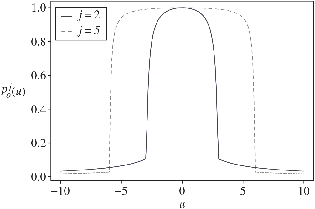
Figure 2. Initial profile
 $\rho^{ j}_0$
.
$\rho^{ j}_0$
.
For example, an initial profile with these attributes is
 $$\rho _0^j\left( {{u \over N}} \right) = \left\{ {\matrix{
{\exp \left\{ {{{ - 1} \over {(u + j + 1)(j + 1 - u)}}} \right\} + 1 - \exp \left\{ {{{ - 1} \over {{{(j + 1)}^2}}}} \right\}} \hfill & {{\rm{for }} - j - 1{\rm{ < }}u{\rm{ < }}j + 1,} \hfill \cr
{1 - \exp \left\{ {{{ - 1} \over {(j + 1)|u|}}} \right\}} \hfill & {{\rm{otherwise}},} \hfill \cr
} } \right.$$
$$\rho _0^j\left( {{u \over N}} \right) = \left\{ {\matrix{
{\exp \left\{ {{{ - 1} \over {(u + j + 1)(j + 1 - u)}}} \right\} + 1 - \exp \left\{ {{{ - 1} \over {{{(j + 1)}^2}}}} \right\}} \hfill & {{\rm{for }} - j - 1{\rm{ < }}u{\rm{ < }}j + 1,} \hfill \cr
{1 - \exp \left\{ {{{ - 1} \over {(j + 1)|u|}}} \right\}} \hfill & {{\rm{otherwise}},} \hfill \cr
} } \right.$$
for
 $j \geq 1$
a fixed integer. In Figure 2 we show this initial profile for
$j \geq 1$
a fixed integer. In Figure 2 we show this initial profile for
 $j=2$
and
$j=2$
and
 $j=5$
.
$j=5$
.
Let
 $\mu^N$
be a sequence of Bernoulli product measures such that:
$\mu^N$
be a sequence of Bernoulli product measures such that:
 \begin{equation}
\mu^N\{\eta;\ \eta(x)=1\}=\rho^{ j}_0\bigg(\frac{x}{N}\bigg).
\end{equation}
\begin{equation}
\mu^N\{\eta;\ \eta(x)=1\}=\rho^{ j}_0\bigg(\frac{x}{N}\bigg).
\end{equation}
By the above results, the hydrodynamic behaviour of this particle interaction process is described by (2.4) when
 $\lambda=1,$
and by (1.1) when
$\lambda=1,$
and by (1.1) when
 $\lambda \in ( 0,1) $
.
$\lambda \in ( 0,1) $
.
Observe that, when
 $\lambda \in ( 0,1),$
the partial derivatives in the second branch are actually 0, in contrast to Proposition 2.1. This means that, when
$\lambda \in ( 0,1),$
the partial derivatives in the second branch are actually 0, in contrast to Proposition 2.1. This means that, when
 $\lambda =1, \rho$
is discontinuous in each barrier (each macroscopic mark of the Poisson process), but there is passage of the particles in these points and this is governed by Fick’s law. That is, the mass flow in the barriers is proportional to the concentration gradient. On the other hand, if
$\lambda =1, \rho$
is discontinuous in each barrier (each macroscopic mark of the Poisson process), but there is passage of the particles in these points and this is governed by Fick’s law. That is, the mass flow in the barriers is proportional to the concentration gradient. On the other hand, if
 $\lambda \in ( 0,1) $
, a barrier is generated in the continuum, which prevents the passage of particles between the Poisson marks. The macroscopic evolution between the barriers is independent. The heat equation is then obtained with the Neumann boundary condition.
$\lambda \in ( 0,1) $
, a barrier is generated in the continuum, which prevents the passage of particles between the Poisson marks. The macroscopic evolution between the barriers is independent. The heat equation is then obtained with the Neumann boundary condition.
Conditioning on W, let
 $\smash{\rho_{t}^{N,W}(x)=
\mathbb{E}_{\mu^N}[\eta_t(x)]}$
. In order to simplify the notation, we omit the dependence on W of
$\smash{\rho_{t}^{N,W}(x)=
\mathbb{E}_{\mu^N}[\eta_t(x)]}$
. In order to simplify the notation, we omit the dependence on W of
 $\smash{\rho_{t}^{N,W}(x)}$
and we write
$\smash{\rho_{t}^{N,W}(x)}$
and we write
 $\smash{\rho_{t}^N(x)}$
. Then
$\smash{\rho_{t}^N(x)}$
. Then
 $\smash{\rho_{t}^N\colon \mathbb{Z} \rightarrow
[0,1]}$
is the solution of the linear discrete equation
$\smash{\rho_{t}^N\colon \mathbb{Z} \rightarrow
[0,1]}$
is the solution of the linear discrete equation
 \begin{gather}
\partial_t\rho_t^N(x) = N \{c_{x,N}\nabla_N \rho_t^N(x)-c_{x,N}
\nabla_N \rho_t^N(x-1)\},
\\
\rho_0^N(x) = \rho_0^{ j}\bigg(\frac{x}{N}\bigg),
\end{gather}
\begin{gather}
\partial_t\rho_t^N(x) = N \{c_{x,N}\nabla_N \rho_t^N(x)-c_{x,N}
\nabla_N \rho_t^N(x-1)\},
\\
\rho_0^N(x) = \rho_0^{ j}\bigg(\frac{x}{N}\bigg),
\end{gather}
where, for
 $h\colon \mathbb{R} \rightarrow \mathbb{R}, (\nabla_N\;
h)(x)=N[h(x+1)-h(x)]$
and
$h\colon \mathbb{R} \rightarrow \mathbb{R}, (\nabla_N\;
h)(x)=N[h(x+1)-h(x)]$
and
 $c_{x,N}$
is the function defined in (2.2).
$c_{x,N}$
is the function defined in (2.2).
Consider the following time discrete approximation of (2.4). For each
 $N \in \mathbb{N}, \delta >0$
, define
$N \in \mathbb{N}, \delta >0$
, define
 $\smash{\rho_l^{\delta,N}(k)},
\; k \in \mathbb{Z},\; l \geq 0,$
using the following recurrence formula:
$\smash{\rho_l^{\delta,N}(k)},
\; k \in \mathbb{Z},\; l \geq 0,$
using the following recurrence formula:
 \begin{gather}
\begin{aligned}
\rho_{l+1}^{\delta,N}(k) &= \rho_l^{\delta,N}(k)+\delta
N^2[c_{k,N}\rho_l^{\delta,N}(k+1)+c_{k-1,N}\rho_l^{\delta,N}(k-1)
\\
&-(c_{k,N}+c_{k-1,N})\rho_l^{\delta,N}(k)], \nonumber
\end{aligned}
\\
\rho_0^{\delta,N}(k) = \rho_0\bigg(\frac{k}{N}\bigg).
\label{eqn13}\end{gather}
\begin{gather}
\begin{aligned}
\rho_{l+1}^{\delta,N}(k) &= \rho_l^{\delta,N}(k)+\delta
N^2[c_{k,N}\rho_l^{\delta,N}(k+1)+c_{k-1,N}\rho_l^{\delta,N}(k-1)
\\
&-(c_{k,N}+c_{k-1,N})\rho_l^{\delta,N}(k)], \nonumber
\end{aligned}
\\
\rho_0^{\delta,N}(k) = \rho_0\bigg(\frac{k}{N}\bigg).
\label{eqn13}\end{gather}
Therefore, if there exists any Poisson mark between the sites k and
 $k+1$
, then
$k+1$
, then
 \begin{gather}
\rho_{l+1}^{\delta,N}(k)=\rho_l^{\delta,N}(k)+\delta N^2
\bigg[\frac{\lambda}{N}\rho_l^{\delta,N}(k+1)+\rho_l^{\delta,N}
(k-1)-\bigg(1+\frac{\lambda}{N}\bigg)\rho_l^{\delta,N}(k)\bigg],
\\
\rho_{l+1}^{\delta,N}(k+1)=\rho_l^{\delta,N}(k)+\delta N^2
\bigg[\rho_l^{\delta,N}(k+1)+\frac{\lambda}{N}\rho_l^{\delta,N}(k-1)
-\bigg(1+\frac{\lambda}{N}\bigg)\rho_l^{\delta,N}(k)\bigg];
\end{gather}
\begin{gather}
\rho_{l+1}^{\delta,N}(k)=\rho_l^{\delta,N}(k)+\delta N^2
\bigg[\frac{\lambda}{N}\rho_l^{\delta,N}(k+1)+\rho_l^{\delta,N}
(k-1)-\bigg(1+\frac{\lambda}{N}\bigg)\rho_l^{\delta,N}(k)\bigg],
\\
\rho_{l+1}^{\delta,N}(k+1)=\rho_l^{\delta,N}(k)+\delta N^2
\bigg[\rho_l^{\delta,N}(k+1)+\frac{\lambda}{N}\rho_l^{\delta,N}(k-1)
-\bigg(1+\frac{\lambda}{N}\bigg)\rho_l^{\delta,N}(k)\bigg];
\end{gather}
otherwise,
 $c_{k,N}=c_{k-1,N}=c_{k+1,N}=1$
in (2.1.2).
$c_{k,N}=c_{k-1,N}=c_{k+1,N}=1$
in (2.1.2).
On the other hand, by [Reference Jara and Landim7], we fix an initial profile
 $u_0\colon \mathbb{R} \rightarrow \mathbb{R}$
with the fourth derivative bounded and consider
$u_0\colon \mathbb{R} \rightarrow \mathbb{R}$
with the fourth derivative bounded and consider
 $u\colon \mathbb{R}_+ \times \mathbb{R} \rightarrow \mathbb{R}$
as the solution of the heat equation with initial profile
$u\colon \mathbb{R}_+ \times \mathbb{R} \rightarrow \mathbb{R}$
as the solution of the heat equation with initial profile
 $u_0$
, i.e.
$u_0$
, i.e.
 \begin{equation}
\partial_t u(t,x) = \partial^2_xu(t,x),
u(0,x) = u_0(x),
\end{equation}
\begin{equation}
\partial_t u(t,x) = \partial^2_xu(t,x),
u(0,x) = u_0(x),
\end{equation}
and, for each
 $N \in \mathbb{N}$
, we define
$N \in \mathbb{N}$
, we define
 $\smash{u_t^N(x)}$
as the solution of the system of ordinary differential equations
$\smash{u_t^N(x)}$
as the solution of the system of ordinary differential equations
 \begin{equation}
\bigg(\frac{{\rm d}}{{\rm d} t}\bigg)u_t^N(x) = (\Delta_N u_t^N)(x), u_0^N(x)
= u_0\bigg(\frac{x}{N}\bigg),
\end{equation}
\begin{equation}
\bigg(\frac{{\rm d}}{{\rm d} t}\bigg)u_t^N(x) = (\Delta_N u_t^N)(x), u_0^N(x)
= u_0\bigg(\frac{x}{N}\bigg),
\end{equation}
where
 $\Delta_N$
represents the discrete Laplacian. Then, there exists a finite constant
$\Delta_N$
represents the discrete Laplacian. Then, there exists a finite constant
 $C_0> 0$
such that
$C_0> 0$
such that
 \begin{equation}
\bigg|u_t^N(x)-u\bigg(t,\frac{x}{N}\bigg)\bigg| \leq \frac{C_0t}{N^2}
\label{eqn14}
\end{equation}
\begin{equation}
\bigg|u_t^N(x)-u\bigg(t,\frac{x}{N}\bigg)\bigg| \leq \frac{C_0t}{N^2}
\label{eqn14}
\end{equation}
for all
 $N \geq 1, t \geq 0, x \in \mathbb{Z}$
. That is, (2.8) is an approximation of the heat equation by solutions of the discrete heat equation. This approximation introduces our next result.
$N \geq 1, t \geq 0, x \in \mathbb{Z}$
. That is, (2.8) is an approximation of the heat equation by solutions of the discrete heat equation. This approximation introduces our next result.
Proposition 2.3. Let
 $\delta N^2 \lt \smash{\tfrac12}$
. Then there exists a finite constant
$\delta N^2 \lt \smash{\tfrac12}$
. Then there exists a finite constant
 $C(\rho_0) $
such that
$C(\rho_0) $
such that
 \begin{equation}
|\rho_l^{\delta,N}(k)-\rho\bigg(\delta l,\frac{k}{N}\bigg)| \leq
C(\rho_0)\delta l \bigg\{\delta + \frac{1}{N^2}\bigg\} \quad\text{for all
}l \geq 0,
\end{equation}
\begin{equation}
|\rho_l^{\delta,N}(k)-\rho\bigg(\delta l,\frac{k}{N}\bigg)| \leq
C(\rho_0)\delta l \bigg\{\delta + \frac{1}{N^2}\bigg\} \quad\text{for all
}l \geq 0,
\end{equation}
where
 $\rho(\cdot,\cdot) $
is the solution of the diffusion equation with boundaries (2.4) when
$\rho(\cdot,\cdot) $
is the solution of the diffusion equation with boundaries (2.4) when
 $\lambda=1$
.
$\lambda=1$
.
Observe that if
 $l=t/\delta$
and
$l=t/\delta$
and
 $\delta$
goes to 0 then the right-hand side of Proposition 2 is dominated by
$\delta$
goes to 0 then the right-hand side of Proposition 2 is dominated by
 ${C_0t}/{N^2}. $
.
${C_0t}/{N^2}. $
.
Due to the limit above and (2.8), it follows that, for
 $\lambda=1$
and
$\lambda=1$
and
 $\rho_0\colon \mathbb{R} \rightarrow [0,1],$
an initial profile with the fourth derivative limited, there exists a finite constant
$\rho_0\colon \mathbb{R} \rightarrow [0,1],$
an initial profile with the fourth derivative limited, there exists a finite constant
 $C_0>
0$
such that
$C_0>
0$
such that
 \begin{equation}
\bigg|\rho_t^N(x)-\rho\bigg(t,\frac{x}{N}\bigg)\bigg| \leq
\frac{C_0t}{N^2}
\label{eqn15}
\end{equation}
\begin{equation}
\bigg|\rho_t^N(x)-\rho\bigg(t,\frac{x}{N}\bigg)\bigg| \leq
\frac{C_0t}{N^2}
\label{eqn15}
\end{equation}
for all
 $N \geq 1, t \geq 0, x \in \mathbb{T}_N.$
On the other hand, when
 $\lambda \in ( 0,1) $
, then the approximation given in (2.8) is fulfilled since the macroscopic evolution between the barriers is independent and the hydrodynamic limit is given by the weak solution of the heat equation.
$\lambda \in ( 0,1) $
, then the approximation given in (2.8) is fulfilled since the macroscopic evolution between the barriers is independent and the hydrodynamic limit is given by the weak solution of the heat equation.
The following results show the upper and lower bonds of the first displacement time of the tagged particle in the simple exclusion process with random slow bonds given an initial configuration with fourth bounded derivative.
For
 $x,y \in \mathbb{T}_N$
and
$x,y \in \mathbb{T}_N$
and
 $t \geq 0,$
define
$t \geq 0,$
define
 $\smash{\alpha_t^{x,y}}=\lambda t/N$
if there exist a Poisson mark between (x,y) and
$\smash{\alpha_t^{x,y}}=\lambda t/N$
if there exist a Poisson mark between (x,y) and
 $\smash{\alpha_t^{x,y}= t}$
otherwise, and let
$\smash{\alpha_t^{x,y}= t}$
otherwise, and let
 $b(i,k,a,s)= \smash{\sum_{i=\{1,-1\}}\int_a^t\rho_j(s,i/N)}
{\rm d}\alpha_s^{k,0}$
.
$b(i,k,a,s)= \smash{\sum_{i=\{1,-1\}}\int_a^t\rho_j(s,i/N)}
{\rm d}\alpha_s^{k,0}$
.
Theorem 2.1. Fix
 $j \in \mathbb{N}$
and a realization of the process W. Consider an initial profile
$j \in \mathbb{N}$
and a realization of the process W. Consider an initial profile
 $\smash{\rho^{ j}_0}$
with fourth order Taylor’s expansion around the origin that rapidly decreases after
$\smash{\rho^{ j}_0}$
with fourth order Taylor’s expansion around the origin that rapidly decreases after
 $[-j,j]$
.
$[-j,j]$
.
Denote by
 $T_j$
the time when the zero site is empty for the first time. It follows that, for all
$T_j$
the time when the zero site is empty for the first time. It follows that, for all
 $ t\geq 0$
,
$ t\geq 0$
,
1. if there is a slow bond between 0 and 1 or between 0 and
 $-1,$
then
\[
\mathbb{P}_W\{T_j\geq t\}\geq \rho^{ j}_0(0) - t-\frac{\lambda t}{N}-
\frac{C_0t^2(N^2+\lambda^2)}{2N^4}+b(i,i,0,s);
\]
$-1,$
then
\[
\mathbb{P}_W\{T_j\geq t\}\geq \rho^{ j}_0(0) - t-\frac{\lambda t}{N}-
\frac{C_0t^2(N^2+\lambda^2)}{2N^4}+b(i,i,0,s);
\]
2. if there are no slow bonds between the neighbours of 0, then
\[
\mathbb{P}_W\{T_j\geq t\}\geq \rho^{ j}_0(0) - \frac{C_0t^2+2tN^2}{N^2}+
b(i,i,0,s);
\]
3. if there is a slow bond between each of the neighbours of 0, then
\[
\mathbb{P}_W\{T_j\geq t\}\geq \rho^{ j}_0(0) -\frac{\lambda t (C_0\lambda
t+2N^3)}{N^4}+b(i,i,0,s).
\]


Denote by
 ${\rm LB}_k$
the lower bounds stated above, where the subindex k indicates conditions 1, 2, or 3.
${\rm LB}_k$
the lower bounds stated above, where the subindex k indicates conditions 1, 2, or 3.
Theorem 2.2. Fix
 $j \in \mathbb{N}$
and a realization of the process W. Consider the initial profile
$j \in \mathbb{N}$
and a realization of the process W. Consider the initial profile
 $\smash{\rho^{ j}_0}$
. It follows that, for all
$\smash{\rho^{ j}_0}$
. It follows that, for all
 $t\geq 0,$
1. if there is a slow bond between 0 and 1 or between 0 and
$-1,$
then
\begin{align}
&\mathbb{P}_W\{T_j \geq t\}
\\
&{\begin{gathered}\leq 1- \frac{(1-{\rm LB}_1)^2}{1-{\rm
LB}_1+ {t^2} (N^2(3N^2+2C_0t) +\lambda(3N^3+2C_0\lambda t))/{3N^4} -2
\int_0^t\sum_{i\in\{1,-1\}}b(k,i,s,u){\rm d}\alpha_s^k};\end{gathered}}
\end{align}
2. if there are no slow bonds between the neighbours of 0, then
\begin{align}
&\mathbb{P}_W\{T_j \geq t\}
\\
&\leq 1- \frac{(1-{\rm LB}_2)^2}{1-{\rm LB}_2+ {2} (3N^2t^2+2C_0t^3)/
{3N^2} -2 \int_0^t\sum_{i\in\{1,-1\}}b(k,i,s,u){\rm d}\alpha_s^k};
\end{align}
3. if there is a slow bond between each of the neighbours of 0, then
\begin{align}
&\mathbb{P}_W\{T_j \geq t\}
\\
&\leq 1- \frac{(1-{\rm LB}_3)^2}{1-{\rm LB}_3+ {2} (3N^3\lambda
t^2+2C_0\lambda^2t^3)/{3N^4} -2
\int_0^t\sum_{i\in\{1,-1\}}b(k,i,s,u){\rm d}\alpha_s^k}.
\end{align}


Denote by
 ${\rm UB}_k$
the upper bounds stated above, where the subindex k indicates conditions 1, 2, or 3.
${\rm UB}_k$
the upper bounds stated above, where the subindex k indicates conditions 1, 2, or 3.
With these bounds, it is possible to observe that keeping j fixed, if N grows then
 $T_j$
, the time when the zero site is empty for the first time, grows too, i.e. the decreasing rate of
$T_j$
, the time when the zero site is empty for the first time, grows too, i.e. the decreasing rate of
 $\mathbb{P}_W\{T_j \geq t\}$
is smaller. Furthermore, when t grows, then
$\mathbb{P}_W\{T_j \geq t\}$
is smaller. Furthermore, when t grows, then
 $\mathbb{P}_W\{T_j \geq t\}$
decays quadratically in both the upper and lower bounds. Finally, if we fix t and N and compare cases 1, 2, and 3, it follows that
$\mathbb{P}_W\{T_j \geq t\}$
decays quadratically in both the upper and lower bounds. Finally, if we fix t and N and compare cases 1, 2, and 3, it follows that
 $\mathbb{P}_W\{T_j \geq
t\}$
decreases slower for case 3 and fastest for case 2, as expected.
$\mathbb{P}_W\{T_j \geq
t\}$
decreases slower for case 3 and fastest for case 2, as expected.
Theorem 2.3. (Annealed result) Fix
 $j \in \mathbb{N}$
and consider the initial profile
$j \in \mathbb{N}$
and consider the initial profile
 $\smash{\rho^{ j}_0}$
. Integrating out the environment, it follows that, for all
$\smash{\rho^{ j}_0}$
. Integrating out the environment, it follows that, for all
 $t\geq 0,$
 \begin{equation}
\mathbb{P}\{T_j\geq t\}\geq \rho^{ j}_0(0)+b(i,i,0,s) -{\rm e}^{-\lambda}\bigg(2t+
\frac{C_0t^2}{N^2}\bigg) +({\rm e}^{-\lambda}-1)\bigg(\frac{2\lambda
t}{N}+\frac{C_0\lambda^2 t^2}{N^4}\bigg)
\end{equation}
\begin{equation}
\mathbb{P}\{T_j\geq t\}\geq \rho^{ j}_0(0)+b(i,i,0,s) -{\rm e}^{-\lambda}\bigg(2t+
\frac{C_0t^2}{N^2}\bigg) +({\rm e}^{-\lambda}-1)\bigg(\frac{2\lambda
t}{N}+\frac{C_0\lambda^2 t^2}{N^4}\bigg)
\end{equation}
and
 \begin{equation}
\mathbb{P}\{T_j \geq t\} \leq 2e^{-\lambda}(1-e^{-\lambda}){\rm UB}_1+
{\rm e}^{-2\lambda}{\rm UB}_2+(1-{\rm e}^{-\lambda})^2{\rm UB}_3.
\end{equation}
\begin{equation}
\mathbb{P}\{T_j \geq t\} \leq 2e^{-\lambda}(1-e^{-\lambda}){\rm UB}_1+
{\rm e}^{-2\lambda}{\rm UB}_2+(1-{\rm e}^{-\lambda})^2{\rm UB}_3.
\end{equation}
2.2. The asymptotic behaviour of the random walk
$X_N(t,x) $

Definition 2.1. Let
 $B(t,\omega) $
be a standard Brownian motion defined in some probability space
$B(t,\omega) $
be a standard Brownian motion defined in some probability space
 $ (\mathcal{X}, \mathcal{B}, \mathbb{P}) $
. We define the local time
$ (\mathcal{X}, \mathcal{B}, \mathbb{P}) $
. We define the local time
 $L\colon \mathbb{R}^+ \times \mathbb{R} \rightarrow \mathbb{R}^+$
by
$L\colon \mathbb{R}^+ \times \mathbb{R} \rightarrow \mathbb{R}^+$
by
 \begin{equation}
\int_0^ t\textbf{1}_{\{B(s,\cdot ) \in A\}}{\rm d} s=\int_A L(t,x){\rm d} x
\end{equation}
\begin{equation}
\int_0^ t\textbf{1}_{\{B(s,\cdot ) \in A\}}{\rm d} s=\int_A L(t,x){\rm d} x
\end{equation}
for all Borel sets
 $A \subset (-\infty, \infty) $
and all
$A \subset (-\infty, \infty) $
and all
 $t \geq 0.$
For simplicity, we denote
 $B(t,\omega) $
by B(t) in the sequence.
$B(t,\omega) $
by B(t) in the sequence.
Definition 2.2. Consider the measure
 $\upsilon_E$
such that the support of
$\upsilon_E$
such that the support of
 $\upsilon_E$
, denoted by
$\upsilon_E$
, denoted by
 $ (\upsilon_E) $
, is the set
$ (\upsilon_E) $
, is the set
 $\{W(x),W(x{-})\colon x \in
\mathbb{R}\},$
where
$\{W(x),W(x{-})\colon x \in
\mathbb{R}\},$
where
 $W(x{-})=\lim_{y \rightarrow x-}W( y) $
and so that
$W(x{-})=\lim_{y \rightarrow x-}W( y) $
and so that
 $\smash{\int f(u)\upsilon({\rm d} u)} = \smash{\int f(W(u)){\rm d} u}$
for all
$\smash{\int f(u)\upsilon({\rm d} u)} = \smash{\int f(W(u)){\rm d} u}$
for all
 $f
\in Cc(R) $
.
$f
\in Cc(R) $
.
For each
 $u \in (\upsilon_E) $
and
$u \in (\upsilon_E) $
and
 $t \geq 0,$
set
$t \geq 0,$
set
 \begin{equation}
\varphi(t\mid u,\upsilon_E)=\int_\mathbb{R} L(t,y-u)\upsilon_E({\rm d} y),
\varphi^{-1}(t\mid u,\upsilon_E)=\sup\{s \geq 0\colon \varphi(s\mid
u,\upsilon_E) \leq t\},
\end{equation}
\begin{equation}
\varphi(t\mid u,\upsilon_E)=\int_\mathbb{R} L(t,y-u)\upsilon_E({\rm d} y),
\varphi^{-1}(t\mid u,\upsilon_E)=\sup\{s \geq 0\colon \varphi(s\mid
u,\upsilon_E) \leq t\},
\end{equation}
and
 \begin{equation}
Z(t\mid u,\upsilon_E)=B (\varphi^{-1}(t\mid u,\upsilon_E)) + u.
\end{equation}
\begin{equation}
Z(t\mid u,\upsilon_E)=B (\varphi^{-1}(t\mid u,\upsilon_E)) + u.
\end{equation}
For each
 $u \in (\upsilon_E), \varphi(t\mid u,\upsilon_E) $
is a nondecreasing continuous function on t, strictly positive for
$u \in (\upsilon_E), \varphi(t\mid u,\upsilon_E) $
is a nondecreasing continuous function on t, strictly positive for
 $t>0$
.
$t>0$
.
 $\varphi^{-1}$
is a nondecreasing càdlàg function and
$\varphi^{-1}$
is a nondecreasing càdlàg function and
 $\varphi^{-1}(0,u)=0$
. As a function of time t, the process
$\varphi^{-1}(0,u)=0$
. As a function of time t, the process
 $Z=\{Z(t\mid u,\upsilon_E)\colon t\geq 0\}$
is càdlàg, and it is defined on the same probability space as the Brownian motion B(t), the space
$Z=\{Z(t\mid u,\upsilon_E)\colon t\geq 0\}$
is càdlàg, and it is defined on the same probability space as the Brownian motion B(t), the space
 $ ( (\upsilon_E), \mathcal{B},\mathbb{P}) $
. Also, Z is a strong Markov process with state space
$ ( (\upsilon_E), \mathcal{B},\mathbb{P}) $
. Also, Z is a strong Markov process with state space
 $ (\upsilon_E) $
and initial state u. Furthermore, Z is a birth and death process. See [Reference Stone15] for more details.
$ (\upsilon_E) $
and initial state u. Furthermore, Z is a birth and death process. See [Reference Stone15] for more details.
For
 $N \geq 1$
, let
$N \geq 1$
, let
 $\upsilon_N= ({1}/{N}) \smash{\sum_{x \in
\mathbb{Z}}\delta_{W(x/N)}}$
, and note that
$\upsilon_N= ({1}/{N}) \smash{\sum_{x \in
\mathbb{Z}}\delta_{W(x/N)}}$
, and note that
 $\upsilon_N$
converges vaguely to
$\upsilon_N$
converges vaguely to
 $\upsilon_E$
.
$\upsilon_E$
.
It follows from [Reference Stone15] that, if
 $\{u_i\}_{i \in \mathbb{Z}}$
is a strictly increasing sequence of real numbers such that
$\{u_i\}_{i \in \mathbb{Z}}$
is a strictly increasing sequence of real numbers such that
 $\lim_{i
\rightarrow \pm \infty}u_i=\pm \infty$
and we define
$\lim_{i
\rightarrow \pm \infty}u_i=\pm \infty$
and we define
 $\upsilon=
\smash{\sum_{i \in \mathbb{Z}}w_i\delta_{u_i}},$
where
$\upsilon=
\smash{\sum_{i \in \mathbb{Z}}w_i\delta_{u_i}},$
where
 $\{w_i\}_{i \in \mathbb{Z}}$
are fixed, then
$\{w_i\}_{i \in \mathbb{Z}}$
are fixed, then
 $Z(\cdot \mid u_j,\upsilon) $
is a continuous-time random walk in
$Z(\cdot \mid u_j,\upsilon) $
is a continuous-time random walk in
 $\{u_i\}_{i \in \mathbb{Z}}$
starting at
$\{u_i\}_{i \in \mathbb{Z}}$
starting at
 $u_j$
such that, after reaching site
$u_j$
such that, after reaching site
 $u_i$
, it jumps to
$u_i$
, it jumps to
 $u_{i-1}$
and
$u_{i-1}$
and
 $u_{i+1}$
with respective rates
$u_{i+1}$
with respective rates
 \[
\frac{1}{w_i(u_i-u_{i-1})} \quad\text{and}\quad
\frac{1}{w_i(u_{i+1}-u_i)}.
\]
\[
\frac{1}{w_i(u_i-u_{i-1})} \quad\text{and}\quad
\frac{1}{w_i(u_{i+1}-u_i)}.
\]
Because of the definition of
 $\upsilon_N$
and the last result, the random walk
$\upsilon_N$
and the last result, the random walk
 $X_N(\cdot ,x)/N$
has the same law as the process
$X_N(\cdot ,x)/N$
has the same law as the process
 $W^{-1}(Z(\cdot\mid W(x/N),\upsilon_N)) $
. So, for all
$W^{-1}(Z(\cdot\mid W(x/N),\upsilon_N)) $
. So, for all
 $x \in \mathbb{R}$
, let
$x \in \mathbb{R}$
, let
 \[
Y_N(t,x)=W^ {-1}\bigg(Z\bigg(t\biggm| W\bigg(\frac{\lceil xN\rceil
}{N}\bigg),\upsilon_N\bigg)\bigg),
\]
\[
Y_N(t,x)=W^ {-1}\bigg(Z\bigg(t\biggm| W\bigg(\frac{\lceil xN\rceil
}{N}\bigg),\upsilon_N\bigg)\bigg),
\]
where
 $\lceil xN\rceil $
is the greatest integer less than or equal to xN. It follows that
$\lceil xN\rceil $
is the greatest integer less than or equal to xN. It follows that
 \[
\frac{X_N(\cdot,\lceil xN\rceil)}{N } \quad\text{has the same law as }
Y_N(\cdot,x) \text{ for all $N\geq 1$.}
\]
\[
\frac{X_N(\cdot,\lceil xN\rceil)}{N } \quad\text{has the same law as }
Y_N(\cdot,x) \text{ for all $N\geq 1$.}
\]
On the other hand, note that
 $ (\upsilon_N) $
consists of values of
$ (\upsilon_N) $
consists of values of
 $W(x/N) $
. Let
$W(x/N) $
. Let
 $y_N =W(\lceil uN\rceil/N) $
and
$y_N =W(\lceil uN\rceil/N) $
and
 $d_S$
be the Skorokhod ’s metric in the Skorokhod space
$d_S$
be the Skorokhod ’s metric in the Skorokhod space
 $D(I\subset \mathbb{R},\mathbb{R}) $
. Let
$D(I\subset \mathbb{R},\mathbb{R}) $
. Let
 $W(\lceil
uN\rceil/N)\rightarrow W(u) $
on the metric
$W(\lceil
uN\rceil/N)\rightarrow W(u) $
on the metric
 $d_S$
as
$d_S$
as
 $N \rightarrow
\infty$
. Then, there exists a sequence of continuous functions
$N \rightarrow
\infty$
. Then, there exists a sequence of continuous functions
 $h_N\colon
\mathbb{R} \rightarrow \mathbb{R}$
such that, for all compact sets
$h_N\colon
\mathbb{R} \rightarrow \mathbb{R}$
such that, for all compact sets
 $K \subset \mathbb{R}$
,
$K \subset \mathbb{R}$
,
 \[
\lim_{N \rightarrow \infty}\sup_{u \in K}|u-h_N(u)|=0
\]
\[
\lim_{N \rightarrow \infty}\sup_{u \in K}|u-h_N(u)|=0
\]
and
 \[
\lim_{N \rightarrow \infty}\sup_{u \in K}\bigg|W\bigg(\frac{\lceil
uN\rceil}{N}\bigg)-W(h_N(u))\bigg|=0.
\]
\[
\lim_{N \rightarrow \infty}\sup_{u \in K}\bigg|W\bigg(\frac{\lceil
uN\rceil}{N}\bigg)-W(h_N(u))\bigg|=0.
\]
This implies that
 $y_N \rightarrow y,$
where
$y_N \rightarrow y,$
where
 $y= W(u) $
or
$y= W(u) $
or
 $W(u{-}),$
and, therefore,
$W(u{-}),$
and, therefore,
 $y \in (\upsilon _E) $
.
$y \in (\upsilon _E) $
.
Since
 $\lim_{N \uparrow \infty}W(\lceil xN\rceil/N) =W(x) $
and
$\lim_{N \uparrow \infty}W(\lceil xN\rceil/N) =W(x) $
and
 $\upsilon_N$
converges vaguely to
$\upsilon_N$
converges vaguely to
 $\upsilon _E$
, then
$\upsilon _E$
, then
 \begin{equation}
\lim_{N \uparrow \infty}d_S\bigg(Z\bigg(\cdot\biggm| W\bigg(\frac{\lceil
xN\rceil}{N}\bigg),\upsilon_N\bigg),Z(\cdot\mid W(x),\upsilon
\textbf{1}_{\{E\}})\bigg)=0 \quad\text{almost surely (a.s.)}.
\end{equation}
\begin{equation}
\lim_{N \uparrow \infty}d_S\bigg(Z\bigg(\cdot\biggm| W\bigg(\frac{\lceil
xN\rceil}{N}\bigg),\upsilon_N\bigg),Z(\cdot\mid W(x),\upsilon
\textbf{1}_{\{E\}})\bigg)=0 \quad\text{almost surely (a.s.)}.
\end{equation}
Note that two trajectories in the Skorokhod topology are close if in any limited time interval these trajectories are uniformly close after a small distortion on the time axis. In the subspace of continuous functions, convergence in the metric
 $ d_S $
is the same as uniform convergence on compact intervals.
$ d_S $
is the same as uniform convergence on compact intervals.
2.3. The jump function W and the operator
$ ({{\rm d}}/{{\rm d} x}) ({{\rm d}}/{{\rm d} W}) $

Consider the process Y(t,x) with
 $t\geq 0$
and
$t\geq 0$
and
 $x \in \mathbb{R}$
defined by
$x \in \mathbb{R}$
defined by
 \begin{equation}
Y(t,x)=W^{-1}(Z(t\mid W(x),\upsilon \textbf{1}_{\{E\}})).
\end{equation}
\begin{equation}
Y(t,x)=W^{-1}(Z(t\mid W(x),\upsilon \textbf{1}_{\{E\}})).
\end{equation}
We find that, for all
 $x \in \mathbb{R}$
,
$x \in \mathbb{R}$
,
 \begin{equation}
\lim_{N\rightarrow \infty}d_S(Y_N(\cdot ,x)-Y(\cdot ,x))=0
\quad\text{a.s.}
\end{equation}
\begin{equation}
\lim_{N\rightarrow \infty}d_S(Y_N(\cdot ,x)-Y(\cdot ,x))=0
\quad\text{a.s.}
\end{equation}
Moreover,
 $Y(\cdot ,x) $
has continuous paths a.s., and, for all
$Y(\cdot ,x) $
has continuous paths a.s., and, for all
 $x \in
\mathbb{R}$
and
$x \in
\mathbb{R}$
and
 $T>0$
,
$T>0$
,
 \begin{equation}
\lim_{N \rightarrow \infty}\sup_{0 \leq t \leq T}|Y_N(t,x)-Y(t,x)|=0
\quad\text{a.s.}
\label{eqn16}
\end{equation}
\begin{equation}
\lim_{N \rightarrow \infty}\sup_{0 \leq t \leq T}|Y_N(t,x)-Y(t,x)|=0
\quad\text{a.s.}
\label{eqn16}
\end{equation}
Our objective now is to study the Markov process
 $Z(t\mid u,\upsilon_E) $
. Note that
$Z(t\mid u,\upsilon_E) $
. Note that
 \begin{equation}
Z(t\mid u,\upsilon _E)=B(\varphi^{-1}(t,u,\upsilon _E)) + u
\end{equation}
\begin{equation}
Z(t\mid u,\upsilon _E)=B(\varphi^{-1}(t,u,\upsilon _E)) + u
\end{equation}
is a process with space states
 $ (\upsilon_E)=\{W(x),W(x{-})\colon x \in
\mathbb{R}\}$
. We study the functions that belong to the domain
$ (\upsilon_E)=\{W(x),W(x{-})\colon x \in
\mathbb{R}\}$
. We study the functions that belong to the domain
 $\smash{\mathcal{D}_{W}^Z}$
of the Z process generator and denote by
$\smash{\mathcal{D}_{W}^Z}$
of the Z process generator and denote by
 $\smash{\mathcal{L}_{W}^Z}$
its generator.
$\smash{\mathcal{L}_{W}^Z}$
its generator.
Denote by
 $\{S(t)\colon t \geq 0\}$
the Markov semigroup associated to
$\{S(t)\colon t \geq 0\}$
the Markov semigroup associated to
 $Z(t\mid u,\upsilon_E) $
, i.e.
$Z(t\mid u,\upsilon_E) $
, i.e.
 \begin{equation}
S(t) f(u)=\mathbb{E}[\,f(Z(t\mid u,\upsilon_E))]
\end{equation}
\begin{equation}
S(t) f(u)=\mathbb{E}[\,f(Z(t\mid u,\upsilon_E))]
\end{equation}
for all
 $f \in C_0(\{W(x),W(x{-})\colon x \in \mathbb{R}\}) $
. Consider the transition density function p of the Markov process
$f \in C_0(\{W(x),W(x{-})\colon x \in \mathbb{R}\}) $
. Consider the transition density function p of the Markov process
 $Z(t\mid
u,\upsilon_E) $
defined on
$Z(t\mid
u,\upsilon_E) $
defined on
 $ (0,\infty) \times (\upsilon_E) $
.
$ (0,\infty) \times (\upsilon_E) $
.
It is known that, for
 $u \in (\upsilon_E) $
and
$u \in (\upsilon_E) $
and
 $\delta > 0$
,
$\delta > 0$
,
1.
$\smash{\lim_{t \rightarrow 0}t^{-1}[1-\int_{|u-w|\lt\delta}p(t,u,w)
\upsilon _E({\rm d} w)]}=0;$
2.
$\smash{\lim_{t \rightarrow 0}t^{-1}\int_{|u-w|\lt\delta}(w-u)p(t,u,w)
\upsilon _E({\rm d} w)}= b(u);$
3.
$\smash{\lim_{t \rightarrow 0}t^{-1}\int_{|u-w|\lt\delta}(u-w)^2p(t,u,w)
\upsilon _E({\rm d} w)}=2a(u);$
4.for all
$f \in C_0( (\upsilon_E)) $
with second continuous derivative,


 \begin{equation}
\lim_{t \rightarrow 0}t^{-1}\bigg[\int f(w)p(t,u,w)\upsilon
\textbf{1}_{\{E\}}({\rm d} w)-f(u)\bigg]=a(u) f''(u)+b(u) f'(u),
\end{equation}
\begin{equation}
\lim_{t \rightarrow 0}t^{-1}\bigg[\int f(w)p(t,u,w)\upsilon
\textbf{1}_{\{E\}}({\rm d} w)-f(u)\bigg]=a(u) f''(u)+b(u) f'(u),
\end{equation}
where a and b are the diffusion and drift coefficients, respectively [Reference Mandl11].
Because of the latter conditions, we observe that there exists a close relationship between the generator
 $\mathcal{L}_{W}^Z$
and the differential operator
$\mathcal{L}_{W}^Z$
and the differential operator
 $a(u)({{\rm d}^2}/{{\rm d} u^2})+b(u)({{\rm d}}/{{\rm d} u}) $
. Formally we can write
$a(u)({{\rm d}^2}/{{\rm d} u^2})+b(u)({{\rm d}}/{{\rm d} u}) $
. Formally we can write
 \begin{equation}
a(u)\frac{{\rm d}^2}{{\rm d} u^2}+b(u)\frac{{\rm d}}{{\rm d} u}=\frac{{\rm d}}{{\rm d}\upsilon
_E} \frac{{\rm d}}{{\rm d} u},
\end{equation}
\begin{equation}
a(u)\frac{{\rm d}^2}{{\rm d} u^2}+b(u)\frac{{\rm d}}{{\rm d} u}=\frac{{\rm d}}{{\rm d}\upsilon
_E} \frac{{\rm d}}{{\rm d} u},
\end{equation}
where the generalized derivative of a real function f with respect to
 $\upsilon _E$
is
$\upsilon _E$
is
 \begin{equation}
\frac{{\rm d}\ f}{{\rm d}\upsilon _E}(x)=\lim_{y \rightarrow x}\frac{f( y)-f(x)}
{\upsilon _E( y)-\upsilon _E(x)},
\end{equation}
\begin{equation}
\frac{{\rm d}\ f}{{\rm d}\upsilon _E}(x)=\lim_{y \rightarrow x}\frac{f( y)-f(x)}
{\upsilon _E( y)-\upsilon _E(x)},
\end{equation}
provided the limit exists.
Let
 $f,g \in C_0( (\upsilon_E)) $
such that
$f,g \in C_0( (\upsilon_E)) $
such that
 \begin{equation}
g(u)=\frac{{\rm d}}{{\rm d}\upsilon _E}\frac{{\rm d}}{{\rm d}
u}\,f(u)=\mathcal{L}_{W}^Z\,f(u).
\end{equation}
\begin{equation}
g(u)=\frac{{\rm d}}{{\rm d}\upsilon _E}\frac{{\rm d}}{{\rm d}
u}\,f(u)=\mathcal{L}_{W}^Z\,f(u).
\end{equation}
Therefore,
 \begin{equation}
f(u)=\int_0^u\int_0^wg(a)\upsilon_E({\rm d} a){\rm d} w + f(0)+uf'(0).
\label{eqn17}
\end{equation}
\begin{equation}
f(u)=\int_0^u\int_0^wg(a)\upsilon_E({\rm d} a){\rm d} w + f(0)+uf'(0).
\label{eqn17}
\end{equation}
In view of this,
 $\smash{\mathcal{D}_{W}^Z}$
is the set of functions
$\smash{\mathcal{D}_{W}^Z}$
is the set of functions
 $f
\in C_0( (\upsilon_E)) $
such that f’(u) are differentiable on
$f
\in C_0( (\upsilon_E)) $
such that f’(u) are differentiable on
 $\upsilon_E$
, for which there is
$\upsilon_E$
, for which there is
 $g \in C_0( (\upsilon_E)) $
that satisfies (2.11). Therefore,
$g \in C_0( (\upsilon_E)) $
that satisfies (2.11). Therefore,
 $\smash{\mathcal{L}_{W}^Z\colon
\mathcal{D}_{W}^Z} \rightarrow C_0( (\upsilon_E)) $
is the generator of the semigroup
$\smash{\mathcal{L}_{W}^Z\colon
\mathcal{D}_{W}^Z} \rightarrow C_0( (\upsilon_E)) $
is the generator of the semigroup
 $\{S(t)\colon t \geq 0\}$
and
$\{S(t)\colon t \geq 0\}$
and
 \begin{equation}
\mathcal{L}_{W}^Z=\frac{{\rm d}}{{\rm d} \upsilon_E}\frac{{\rm d}}{{\rm d} u}.
\end{equation}
\begin{equation}
\mathcal{L}_{W}^Z=\frac{{\rm d}}{{\rm d} \upsilon_E}\frac{{\rm d}}{{\rm d} u}.
\end{equation}
As discussed in [Reference Faggionato, Jara and Landim1], the process
 $Y(t,u)=Y_t$
is not strongly Markov with respect to the filtration
$Y(t,u)=Y_t$
is not strongly Markov with respect to the filtration
 $
\mathcal{F}_t^Y=\sigma(Y_s\colon s \leq t) $
and, in particular, it is not a Feller Markov process.
$
\mathcal{F}_t^Y=\sigma(Y_s\colon s \leq t) $
and, in particular, it is not a Feller Markov process.
Let
 $\{\gamma_j\colon j\in \mathbb{R}\}$
be the sequence of Poisson marks on
$\{\gamma_j\colon j\in \mathbb{R}\}$
be the sequence of Poisson marks on
 $\mathbb{R},$
i.e. the jump points of W. We have that
$\mathbb{R},$
i.e. the jump points of W. We have that
 \begin{equation}
W^{-1}(W(\gamma_j))=W^{-1}(W(\gamma_j{-})).
\end{equation}
\begin{equation}
W^{-1}(W(\gamma_j))=W^{-1}(W(\gamma_j{-})).
\end{equation}
To obtain the generator of the process
 $Y_t$
, we divide each jump point of W in two, i.e. we consider the sets
$Y_t$
, we divide each jump point of W in two, i.e. we consider the sets
 $\{\gamma_j\colon j\in \mathbb{R}\}$
and
$\{\gamma_j\colon j\in \mathbb{R}\}$
and
 $\smash{\{\gamma_j^-\colon j\in \mathbb{R}\}},$
and the bijective function
$\smash{\{\gamma_j^-\colon j\in \mathbb{R}\}},$
and the bijective function
 $W_b\colon \mathbb{R} \smash{\cup \{\gamma_j^-}\,{\colon} j\in \mathbb{R}\} \rightarrow
(\upsilon_E) $
such that
$W_b\colon \mathbb{R} \smash{\cup \{\gamma_j^-}\,{\colon} j\in \mathbb{R}\} \rightarrow
(\upsilon_E) $
such that
 $W_b(x)=W(x) $
for
$W_b(x)=W(x) $
for
 $x \in \mathbb{R}$
, and
$x \in \mathbb{R}$
, and
 $W_b(\gamma_j^{-})=W(\gamma_j{-}) $
for
$W_b(\gamma_j^{-})=W(\gamma_j{-}) $
for
 $j \in \mathbb{R}$
. The inverse function
$j \in \mathbb{R}$
. The inverse function
 $\smash{W_b^{-1}\colon (\upsilon_E)} \rightarrow \mathbb{R} \smash{\cup
\{\gamma_j^-}\colon j\in \mathbb{R}\}$
is given by
$\smash{W_b^{-1}\colon (\upsilon_E)} \rightarrow \mathbb{R} \smash{\cup
\{\gamma_j^-}\colon j\in \mathbb{R}\}$
is given by
 $\smash{W_b^{-1}(W(x))}=x,\smash{W_b^{-1}(W(\gamma_j{-}))=\gamma_j^-}$
.
$\smash{W_b^{-1}(W(x))}=x,\smash{W_b^{-1}(W(\gamma_j{-}))=\gamma_j^-}$
.
Consider the spaces
 $ (\mathbb{R} \smash{\cup \{\gamma_j^-}\colon j\in \mathbb{R}\},
d_{W_B}) $
and
$ (\mathbb{R} \smash{\cup \{\gamma_j^-}\colon j\in \mathbb{R}\},
d_{W_B}) $
and
 $ ( (\upsilon_E),d) $
, where
$ ( (\upsilon_E),d) $
, where
 $d_{W_B}$
is defined by
$d_{W_B}$
is defined by
 \begin{equation}
d_{W_B}(\gamma_j^-,\gamma_k^{-})=|W(\gamma_j{-})-W(\gamma_k{-})|, \qquad
d_{W_B}(\gamma_j^-,y)=|W(\gamma_j{-})-W( y)|,
\end{equation}
\begin{equation}
d_{W_B}(\gamma_j^-,\gamma_k^{-})=|W(\gamma_j{-})-W(\gamma_k{-})|, \qquad
d_{W_B}(\gamma_j^-,y)=|W(\gamma_j{-})-W( y)|,
\end{equation}
and d is the Euclidean distance. Then
 $W_b$
is an isometry between the two spaces defined above. Hence, all the results concerning the process Z can be restated in terms of the process
$W_b$
is an isometry between the two spaces defined above. Hence, all the results concerning the process Z can be restated in terms of the process
 $U_t=\smash{W_b^{-1}(Z_t)}$
with space state
$U_t=\smash{W_b^{-1}(Z_t)}$
with space state
 $\mathbb{R} \smash{\cup} \{\gamma_j^-\colon j\in \mathbb{R}\} $
. The domain of the
$\mathbb{R} \smash{\cup} \{\gamma_j^-\colon j\in \mathbb{R}\} $
. The domain of the
 $U_t$
generator,
$U_t$
generator,
 $\smash{\mathcal{L}_{W}^U}$
, denoted by
$\smash{\mathcal{L}_{W}^U}$
, denoted by
 $\smash{\mathcal{D}_{W}^U}$
is given by
$\smash{\mathcal{D}_{W}^U}$
is given by
 \begin{equation}
\mathcal{D}_{W}^U=\{ f\circ W_b\colon f \in \mathcal{D}_{W}^Z\},
\end{equation}
\begin{equation}
\mathcal{D}_{W}^U=\{ f\circ W_b\colon f \in \mathcal{D}_{W}^Z\},
\end{equation}
where, as usual,
 $f\circ W_b$
denotes the composition of f with
$f\circ W_b$
denotes the composition of f with
 $W_b$
.
$W_b$
.
Let
 $f,g \in C_0( (\upsilon_E)) $
with
$f,g \in C_0( (\upsilon_E)) $
with
 $c=f(0) $
and
$c=f(0) $
and
 $e=f'(0) $
such that
$e=f'(0) $
such that
 \begin{equation}
f(u)=\int_0^u\int_0^wg(a)\upsilon_E({\rm d} a){\rm d} w + c+ ue.
\end{equation}
\begin{equation}
f(u)=\int_0^u\int_0^wg(a)\upsilon_E({\rm d} a){\rm d} w + c+ ue.
\end{equation}
By a change of variables, we have
 \[
f(W_b(x))=\int_0^{W_b(x)}\int_0^{W_b( y)}g(W_b(z)){\rm d} W^{-1}(W_b(z)) {\rm d}
W_b( y)+ c+W_b(x)\,e.
\]
\[
f(W_b(x))=\int_0^{W_b(x)}\int_0^{W_b( y)}g(W_b(z)){\rm d} W^{-1}(W_b(z)) {\rm d}
W_b( y)+ c+W_b(x)\,e.
\]
So, for
 $x \in \mathbb{R}$
, we have
$x \in \mathbb{R}$
, we have
 \[
f\circ W_b (x)=\int_0^{x}\int_0^{y}g\circ W_b(z){\rm d}(z) {\rm d} W( y)+
c+W(x)\,e,
\]
\[
f\circ W_b (x)=\int_0^{x}\int_0^{y}g\circ W_b(z){\rm d}(z) {\rm d} W( y)+
c+W(x)\,e,
\]
and, writing
 $F= f\circ W_b$
and
$F= f\circ W_b$
and
 $G= g\circ W_b$
, we obtain
$G= g\circ W_b$
, we obtain
 \begin{equation}
F (x)=\int_0^{x}\int_0^{y}G(z){\rm d}(z) {\rm d} W( y)+ c+eW(x).
\label{eqn18}
\end{equation}
\begin{equation}
F (x)=\int_0^{x}\int_0^{y}G(z){\rm d}(z) {\rm d} W( y)+ c+eW(x).
\label{eqn18}
\end{equation}
By continuity in
 $\mathbb{R}$
,
$\mathbb{R}$
,
 \begin{equation}
F(\gamma_j^{-})=F(\gamma_j{-}) \quad\text{for all } j \in \mathbb{R}.
\end{equation}
\begin{equation}
F(\gamma_j^{-})=F(\gamma_j{-}) \quad\text{for all } j \in \mathbb{R}.
\end{equation}
It follows that
 $\smash{\mathcal{D}_{W}^U}$
is the set of functions
$\smash{\mathcal{D}_{W}^U}$
is the set of functions
 $F
\in C_0(\mathbb{R} \cup \{\gamma_j^-\colon j\in \mathbb{R}\}) $
for which there exists
$F
\in C_0(\mathbb{R} \cup \{\gamma_j^-\colon j\in \mathbb{R}\}) $
for which there exists
 $G \in C_0(\mathbb{R} \cup \{\gamma_j^-\colon j\in \mathbb{R}\}) $
and where (2.12) is satisfied. Therefore,
$G \in C_0(\mathbb{R} \cup \{\gamma_j^-\colon j\in \mathbb{R}\}) $
and where (2.12) is satisfied. Therefore,
 \begin{equation}
\mathcal{L}_{W}^U=\frac{{\rm d}}{{\rm d} x}\frac{{\rm d}}{{\rm d} W}
\quad\textrm{and}\quad \mathcal{L}_{W}^U\,F=G.
\end{equation}
\begin{equation}
\mathcal{L}_{W}^U=\frac{{\rm d}}{{\rm d} x}\frac{{\rm d}}{{\rm d} W}
\quad\textrm{and}\quad \mathcal{L}_{W}^U\,F=G.
\end{equation}
We now turn to the process
 $Y_t=Y(t,x) $
. Denote by
$Y_t=Y(t,x) $
. Denote by
 $\{T(t)\colon t \geq
0\}$
the semigroup of the Markov process
$\{T(t)\colon t \geq
0\}$
the semigroup of the Markov process
 $Y_t$
. Let
$Y_t$
. Let
 $C_{W,0}(\mathbb{R}) $
be the set of bounded càdlàg functions which vanish at
$C_{W,0}(\mathbb{R}) $
be the set of bounded càdlàg functions which vanish at
 $\pm \infty$
, whose discontinuities form a subset of the set of jump points of W. Let
$\pm \infty$
, whose discontinuities form a subset of the set of jump points of W. Let
 $\varphi\colon \mathbb{R} \cup \{\smash{\gamma_j^-}\colon j\in \mathbb{R}\}
\rightarrow \mathbb{R}$
be such that
$\varphi\colon \mathbb{R} \cup \{\smash{\gamma_j^-}\colon j\in \mathbb{R}\}
\rightarrow \mathbb{R}$
be such that
 $\varphi(x)=x$
for all
$\varphi(x)=x$
for all
 $x \in \mathbb{R}$
and
$x \in \mathbb{R}$
and
 $\varphi(\gamma_j^{-})=\gamma_j$
for all
$\varphi(\gamma_j^{-})=\gamma_j$
for all
 $j \in \mathbb{R}$
. We have
$j \in \mathbb{R}$
. We have
 $Y_t=\varphi(U_t) $
.
$Y_t=\varphi(U_t) $
.
Given a function
 $H\colon \mathbb{R} \rightarrow \mathbb{R}$
, we define the function
$H\colon \mathbb{R} \rightarrow \mathbb{R}$
, we define the function
 \begin{equation}
H \circ \varphi\colon \mathbb{R} \cup \{\gamma_j^-\colon j\in \mathbb{R}\}
\rightarrow \mathbb{R}
\end{equation}
\begin{equation}
H \circ \varphi\colon \mathbb{R} \cup \{\gamma_j^-\colon j\in \mathbb{R}\}
\rightarrow \mathbb{R}
\end{equation}
to obtain
 \begin{equation}
\mathcal{L}_{W}^Y H=\mathcal{L}_{W}^UH \circ \varphi, \qquad H \in
\mathcal{D}_{W}^Y,
\end{equation}
\begin{equation}
\mathcal{L}_{W}^Y H=\mathcal{L}_{W}^UH \circ \varphi, \qquad H \in
\mathcal{D}_{W}^Y,
\end{equation}
where
 $\smash{\mathcal{D}_{W}^Y}$
is the set of functions
$\smash{\mathcal{D}_{W}^Y}$
is the set of functions
 $H \in
C_{W,0}(\mathbb{R}) $
for which there exists
$H \in
C_{W,0}(\mathbb{R}) $
for which there exists
 $G \in C_{W,0}(\mathbb{R}) $
and constants
$G \in C_{W,0}(\mathbb{R}) $
and constants
 $c,e \in \mathbb{R}$
satisfying the equation
$c,e \in \mathbb{R}$
satisfying the equation
 \begin{equation}
H (x)=\int_0^{x}\int_0^{y}G(z){\rm d}(z) {\rm d} W( y)+ c+eW(x), \qquad x \in
\mathbb{R}.
\label{eqn19}
\end{equation}
\begin{equation}
H (x)=\int_0^{x}\int_0^{y}G(z){\rm d}(z) {\rm d} W( y)+ c+eW(x), \qquad x \in
\mathbb{R}.
\label{eqn19}
\end{equation}
Hence, considering the linear operator
 $\mathcal{L}_{W}^Y\colon
\mathcal{D}_{W}^Y \rightarrow C_{W,0}(\mathbb{R}) $
given by
$\mathcal{L}_{W}^Y\colon
\mathcal{D}_{W}^Y \rightarrow C_{W,0}(\mathbb{R}) $
given by
 \begin{equation}
\mathcal{L}_{W}^YH=\frac{{\rm d}}{{\rm d} x}\frac{{\rm d}}{{\rm d} W}H=G,
\end{equation}
\begin{equation}
\mathcal{L}_{W}^YH=\frac{{\rm d}}{{\rm d} x}\frac{{\rm d}}{{\rm d} W}H=G,
\end{equation}
and using (2.13), we find that H satisfies
 \begin{equation}
\frac{\partial H}{\partial x}(\gamma_j{+})=\frac{\partial H} {\partial
x}(\gamma_j{-})
\end{equation}
\begin{equation}
\frac{\partial H}{\partial x}(\gamma_j{+})=\frac{\partial H} {\partial
x}(\gamma_j{-})
\end{equation}
and
 \begin{equation}
\frac{\partial H}{\partial x}(\gamma_j{+})=\lambda [H(\gamma_j{+})
-H(\gamma_j{-})].
\end{equation}
\begin{equation}
\frac{\partial H}{\partial x}(\gamma_j{+})=\lambda [H(\gamma_j{+})
-H(\gamma_j{-})].
\end{equation}
See [Reference Mandl11] for more details.
3. Proof of the hydrodynamic limit
Proof of Proposition 2.1. For a positive measure
 $\pi$
with finite total mass and for functions
$\pi$
with finite total mass and for functions
 $G
\in C_c(\mathbb{R}) $
, consider the notation
$G
\in C_c(\mathbb{R}) $
, consider the notation
 \begin{equation}
\langle\pi,G\rangle=\int G(u)\pi({\rm d} u).
\end{equation}
\begin{equation}
\langle\pi,G\rangle=\int G(u)\pi({\rm d} u).
\end{equation}
We prove that the empirical measure satisfies (2.4), i.e.
 \begin{equation}
\pi_t^N \rightarrow \pi_t \quad\textrm{when } N\rightarrow \infty
\textrm{ in probability.}
\end{equation}
\begin{equation}
\pi_t^N \rightarrow \pi_t \quad\textrm{when } N\rightarrow \infty
\textrm{ in probability.}
\end{equation}
Let
 $T>0$
, and fix a realization of W and the continuous profile
$T>0$
, and fix a realization of W and the continuous profile
 $\rho_0\colon \mathbb{R} \rightarrow \mathbb{Z}$
. Consider a sequence of probability measures
$\rho_0\colon \mathbb{R} \rightarrow \mathbb{Z}$
. Consider a sequence of probability measures
 $\smash{\mathbb{Q}_{\mu^N}^{W}}$
on the path space
$\smash{\mathbb{Q}_{\mu^N}^{W}}$
on the path space
 $D([0,T],\mathcal{M_+}) $
, beginning in
$D([0,T],\mathcal{M_+}) $
, beginning in
 $\mu^N$
and induced by the process
$\mu^N$
and induced by the process
 $\smash{\pi_t^N }$
, evolving according to the generator
$\smash{\pi_t^N }$
, evolving according to the generator
 \begin{align}
(\mathcal{L_N}f)(\eta)(x)&=
c_x\eta(x)(1-\eta(x+1))\{ f(\sigma^{x,x+1}\eta)-f(\eta)\}\nonumber
\\
& + c_{x-1}\eta(x)(1-\eta(x-1))\{ f(\sigma^{x,x-1}\eta)-f(\eta)\}
\label{eqn20}\end{align}
\begin{align}
(\mathcal{L_N}f)(\eta)(x)&=
c_x\eta(x)(1-\eta(x+1))\{ f(\sigma^{x,x+1}\eta)-f(\eta)\}\nonumber
\\
& + c_{x-1}\eta(x)(1-\eta(x-1))\{ f(\sigma^{x,x-1}\eta)-f(\eta)\}
\label{eqn20}\end{align}
speeded up by
 $N^2$
. Denote by
$N^2$
. Denote by
 $\mathcal{M_+}$
the space of finite positive measures in
$\mathcal{M_+}$
the space of finite positive measures in
 $\mathbb{T}=[0,1) $
and by
$\mathbb{T}=[0,1) $
and by
 $D([0,T],\mathcal{M_+}) $
the space provided with the Skorokhod metric of right-continuous functions with left limits
$D([0,T],\mathcal{M_+}) $
the space provided with the Skorokhod metric of right-continuous functions with left limits
 $f\colon [0,T] \rightarrow \mathbb{R}$
.
$f\colon [0,T] \rightarrow \mathbb{R}$
.
Let
 $\mathbb{Q}^W$
be a probability measure on
$\mathbb{Q}^W$
be a probability measure on
 $D([0,T],\mathcal{M_+}) $
concentrated on the deterministic path
$D([0,T],\mathcal{M_+}) $
concentrated on the deterministic path
 $\pi_t({\rm d} u)=\rho(t,u){\rm d} u$
, where
$\pi_t({\rm d} u)=\rho(t,u){\rm d} u$
, where
 $\rho(t,u)=T(t)\rho_0(u) $
. We prove that
$\rho(t,u)=T(t)\rho_0(u) $
. We prove that
 $\pi_t^N$
converge in distribution to the probability measure
$\pi_t^N$
converge in distribution to the probability measure
 $\mathbb{Q} ^W$
concentrated on the deterministic path
$\mathbb{Q} ^W$
concentrated on the deterministic path
 $\{\rho(t,u){\rm d} u, 0 \leq t \leq T\}$
. Convergence in distribution to a continuous deterministic trajectory implies convergence in probability. So, first we prove that
$\{\rho(t,u){\rm d} u, 0 \leq t \leq T\}$
. Convergence in distribution to a continuous deterministic trajectory implies convergence in probability. So, first we prove that
 $\mathbb{Q}_{\mu^N}^{W}$
is relatively compact and then we characterize the limit points of
$\mathbb{Q}_{\mu^N}^{W}$
is relatively compact and then we characterize the limit points of
 $\mathbb{Q}_{\mu^N}^{W}$
.
$\mathbb{Q}_{\mu^N}^{W}$
.
In order to prove that
 $\smash{\mathbb{Q}_{\mu^N}^{W}}$
is relatively compact, it is enough to show that
$\smash{\mathbb{Q}_{\mu^N}^{W}}$
is relatively compact, it is enough to show that
 $\langle\smash{\pi_t^N},g_k\rangle$
, is relatively compact, where
$\langle\smash{\pi_t^N},g_k\rangle$
, is relatively compact, where
 $\{g_k, k \geq 1\}$
is a dense enumerable subfamily of
$\{g_k, k \geq 1\}$
is a dense enumerable subfamily of
 $C(\mathbb{R}) $
. We introduce the linear bounded operator in
$C(\mathbb{R}) $
. We introduce the linear bounded operator in
 $C_c(\mathbb{R}) $
,
$C_c(\mathbb{R}) $
,
 $\smash{R^N_\alpha=(\alpha-\mathcal{L}_{W}^{Y_N})^{-1}}$
, where
$\smash{R^N_\alpha=(\alpha-\mathcal{L}_{W}^{Y_N})^{-1}}$
, where
 $\smash{R^N_\alpha}$
is the resolvent associated to
$\smash{R^N_\alpha}$
is the resolvent associated to
 $\smash{\mathcal{L}_{W}^{Y_N}}$
, recalling that
$\smash{\mathcal{L}_{W}^{Y_N}}$
, recalling that
 $\smash{
\mathcal{L}_{W}^{Y_N}}$
is the generator associated to the process
$\smash{
\mathcal{L}_{W}^{Y_N}}$
is the generator associated to the process
 $\{Y_N(t)\colon t\geq 0\}$
.
$\{Y_N(t)\colon t\geq 0\}$
.
For all
 $F \in C_c(\mathbb{R}) $
and
$F \in C_c(\mathbb{R}) $
and
 $\alpha >0,$
we have
$\alpha >0,$
we have
 \begin{equation}
R^N_\alpha F=\int_0^\infty {\rm e}^{-\alpha t}T_N(t)F{\rm d} t,
\end{equation}
\begin{equation}
R^N_\alpha F=\int_0^\infty {\rm e}^{-\alpha t}T_N(t)F{\rm d} t,
\end{equation}
where
 $ T_N(t) $
is the semigroup associated to the process
$ T_N(t) $
is the semigroup associated to the process
 $\{Y_N(t)\colon t\geq 0\}$
.
$\{Y_N(t)\colon t\geq 0\}$
.
So, it is enough to show that the sequences of measures corresponding to the process
 $\smash{\langle \pi_t^N,R^N_\alpha F\rangle}$
is relatively compact in
$\smash{\langle \pi_t^N,R^N_\alpha F\rangle}$
is relatively compact in
 $D([0,T],\mathcal{M}_{+}) $
for all
$D([0,T],\mathcal{M}_{+}) $
for all
 $F \in C_c(\mathbb{R}).$
Fix
$F \in C_c(\mathbb{R}).$
Fix
 $F \in
C_c(\mathbb{R}) $
and consider
$F \in
C_c(\mathbb{R}) $
and consider
 $f_{\alpha,N}=\smash{R^N_\alpha F}.$
Denote by
$f_{\alpha,N}=\smash{R^N_\alpha F}.$
Denote by
 $\smash{\mathbb{Q}_{\mu^N}^{W} f_{\alpha,N} ^{-1}}$
the probability measure in
$\smash{\mathbb{Q}_{\mu^N}^{W} f_{\alpha,N} ^{-1}}$
the probability measure in
 $D([0,T],\mathbb{R}).$
Consider
 $\mathcal{L_N}$
, the operator defined in (3.1), and
$\mathcal{L_N}$
, the operator defined in (3.1), and
 $\mathbb{L}_N$
, the operator defined in (2.3). Let
$\mathbb{L}_N$
, the operator defined in (2.3). Let
 $f(\eta_t)=\smash{({1}/{N})\sum_{x \in\mathbb{Z}}F({x}/{N})\eta_t(x)}$
. We obtain
$f(\eta_t)=\smash{({1}/{N})\sum_{x \in\mathbb{Z}}F({x}/{N})\eta_t(x)}$
. We obtain
 \begin{align}
&f(\sigma^{x,x+1}\eta_t)-f(\eta_t)
\\
&= \frac{1}{N}
\bigg[F\bigg(\frac{x+1}{N}\bigg)-F\bigg(\frac{x}{N}\bigg)\bigg] \eta_t(x)
+ \frac{1}{N}\bigg[F\bigg(\frac{x}{N}\bigg)-F\bigg(\frac{x+1}{N}\bigg)
\bigg]\eta_t(x+1).
\end{align}
\begin{align}
&f(\sigma^{x,x+1}\eta_t)-f(\eta_t)
\\
&= \frac{1}{N}
\bigg[F\bigg(\frac{x+1}{N}\bigg)-F\bigg(\frac{x}{N}\bigg)\bigg] \eta_t(x)
+ \frac{1}{N}\bigg[F\bigg(\frac{x}{N}\bigg)-F\bigg(\frac{x+1}{N}\bigg)
\bigg]\eta_t(x+1).
\end{align}
Therefore,
 \begin{align}
\mathcal{L_N}\langle \pi_t^N,F\rangle &= \frac{1}{N}\sum_{x
\in\mathbb{Z}}c_x\bigg\{F\bigg(\frac{x+1}{N}\bigg)-F\bigg(\frac{x}{N}\bigg)
\bigg\}\eta_t(x)
\\
& + \frac{1}{N}\sum_{x
\in\mathbb{Z}}c_{x-1}\bigg\{F\bigg(\frac{x-1}{N}\bigg)-F\bigg(\frac{x}{N}\bigg)
\bigg\}\eta_t(x)
\\
&= N^{-2}\langle \pi_t^N,\mathbb{L}_N F\rangle.
\end{align}
\begin{align}
\mathcal{L_N}\langle \pi_t^N,F\rangle &= \frac{1}{N}\sum_{x
\in\mathbb{Z}}c_x\bigg\{F\bigg(\frac{x+1}{N}\bigg)-F\bigg(\frac{x}{N}\bigg)
\bigg\}\eta_t(x)
\\
& + \frac{1}{N}\sum_{x
\in\mathbb{Z}}c_{x-1}\bigg\{F\bigg(\frac{x-1}{N}\bigg)-F\bigg(\frac{x}{N}\bigg)
\bigg\}\eta_t(x)
\\
&= N^{-2}\langle \pi_t^N,\mathbb{L}_N F\rangle.
\end{align}
Under
 $\smash{\mathbb{Q}_{\mu^N}^{W},}$
the identity
$\smash{\mathbb{Q}_{\mu^N}^{W},}$
the identity
 \begin{equation}
\langle \pi_t^N, f_{\alpha,N}\rangle=\langle \pi_0^N,
f_{\alpha,N}\rangle+\int_0^tN^2\; \mathcal{L_N}\langle \pi_s^N,
f_{\alpha,N}\rangle {\rm d} s +M_t^{\alpha,N}
\end{equation}
\begin{equation}
\langle \pi_t^N, f_{\alpha,N}\rangle=\langle \pi_0^N,
f_{\alpha,N}\rangle+\int_0^tN^2\; \mathcal{L_N}\langle \pi_s^N,
f_{\alpha,N}\rangle {\rm d} s +M_t^{\alpha,N}
\end{equation}
is satisfied, where
 $\smash{M_t^{\alpha,N}}$
is a martingale with respect to the filtration
$\smash{M_t^{\alpha,N}}$
is a martingale with respect to the filtration
 $\mathcal{F}_t=\sigma(\eta_s,s \leq t) $
. It follows that
$\mathcal{F}_t=\sigma(\eta_s,s \leq t) $
. It follows that
 \begin{align}
\langle \pi_t^N, f_{\alpha,N}\rangle & = \langle \pi_0^N,
f_{\alpha,N}\rangle+\int_0^t\langle \pi_s^N,\mathbb{L}_N f_{\alpha,N}\rangle
{\rm d} s +M_t^{\alpha,N} \nonumber
\\
&= \langle \pi_0^N, f_{\alpha,N}\rangle+\int_0^t\{\alpha\langle \pi_s^N,
f_{\alpha,N}\rangle-\langle \pi_s^N, F\rangle\}{\rm d} s +M_t^{\alpha,N}.
\label{eqn21}\end{align}
\begin{align}
\langle \pi_t^N, f_{\alpha,N}\rangle & = \langle \pi_0^N,
f_{\alpha,N}\rangle+\int_0^t\langle \pi_s^N,\mathbb{L}_N f_{\alpha,N}\rangle
{\rm d} s +M_t^{\alpha,N} \nonumber
\\
&= \langle \pi_0^N, f_{\alpha,N}\rangle+\int_0^t\{\alpha\langle \pi_s^N,
f_{\alpha,N}\rangle-\langle \pi_s^N, F\rangle\}{\rm d} s +M_t^{\alpha,N}.
\label{eqn21}\end{align}
In order to prove that
 \begin{equation}
\lim_{\gamma \rightarrow 0}\limsup _{N \rightarrow \infty}\sup_{\tau \in
\mathcal{T}_T, \theta \leq \gamma}\mathbb{Q}_{\mu^N}^W [|\langle
\pi_t^N,R^N_\alpha F\rangle,\langle \pi_{t+\theta}^N,R^N_\alpha
F\rangle|> \epsilon]=0,
\label{eqn22}
\end{equation}
\begin{equation}
\lim_{\gamma \rightarrow 0}\limsup _{N \rightarrow \infty}\sup_{\tau \in
\mathcal{T}_T, \theta \leq \gamma}\mathbb{Q}_{\mu^N}^W [|\langle
\pi_t^N,R^N_\alpha F\rangle,\langle \pi_{t+\theta}^N,R^N_\alpha
F\rangle|> \epsilon]=0,
\label{eqn22}
\end{equation}
where
 $\mathcal{T}_T$
is a family of stopping times bounded by T, and
$\mathcal{T}_T$
is a family of stopping times bounded by T, and
 $0 \leq \theta \leq \gamma$
, the second and third terms of the right-side of (3.2) were analyzed. See [Reference Kipnis and Landim9] for more details.
$0 \leq \theta \leq \gamma$
, the second and third terms of the right-side of (3.2) were analyzed. See [Reference Kipnis and Landim9] for more details.
Define
 $\smash{N_t^{\alpha,N}=(M_t^{\alpha,N})^2-\int_0^tA_s^{\alpha,N}}
{\rm d} s,$
where
$\smash{N_t^{\alpha,N}=(M_t^{\alpha,N})^2-\int_0^tA_s^{\alpha,N}}
{\rm d} s,$
where
 \begin{equation}
A_t^{\alpha,N}=N^2\mathcal{L_N}\langle \pi_t^N,
f_{\alpha,N}\rangle^2-2N^2\langle \pi_t^N,
f_{\alpha,N}\rangle\mathcal{L_N}\langle \pi_t^N, f_{\alpha,N}\rangle.
\end{equation}
\begin{equation}
A_t^{\alpha,N}=N^2\mathcal{L_N}\langle \pi_t^N,
f_{\alpha,N}\rangle^2-2N^2\langle \pi_t^N,
f_{\alpha,N}\rangle\mathcal{L_N}\langle \pi_t^N, f_{\alpha,N}\rangle.
\end{equation}
In this way, we find that
 $\smash{N_t^{\alpha,N}}$
is a martingale. Note that
$\smash{N_t^{\alpha,N}}$
is a martingale. Note that
 $\smash{A_s^{\alpha,N}}$
can be written as
$\smash{A_s^{\alpha,N}}$
can be written as
 \begin{equation}
- \langle \pi_s^N, f_{\alpha,N}\rangle \langle \pi_s^N,\mathbb{L}_N
f_{\alpha,N}\rangle.
\end{equation}
\begin{equation}
- \langle \pi_s^N, f_{\alpha,N}\rangle \langle \pi_s^N,\mathbb{L}_N
f_{\alpha,N}\rangle.
\end{equation}
Hence,
 \begin{align}
A_s^{\alpha,N} &= \bigg[ \sum_{x \in
\mathbb{Z}}c_x\bigg\{ f_{\alpha,N}\bigg(x+\frac{1}{N}\bigg)-\!
f_{\alpha,N}\bigg(\frac{x}{N}\bigg)\bigg\}\{\eta_s(x)-\!\eta_s(x+1)\}
\bigg] \bigg[\sum_{x \in \mathbb{Z}}
f_{\alpha,N}\bigg(\frac{x}{N}\bigg)\eta_s(x)\bigg]\nonumber
\\
&= \frac{1}{N^2}\sum_{x \in \mathbb{Z}}c_x(\nabla_Nf_{\alpha,N})
\bigg(\frac{x}{N}\bigg)^2\{\eta_s(x+1) -\eta_s(x)\}^2,
\label{eqn23}\end{align}
\begin{align}
A_s^{\alpha,N} &= \bigg[ \sum_{x \in
\mathbb{Z}}c_x\bigg\{ f_{\alpha,N}\bigg(x+\frac{1}{N}\bigg)-\!
f_{\alpha,N}\bigg(\frac{x}{N}\bigg)\bigg\}\{\eta_s(x)-\!\eta_s(x+1)\}
\bigg] \bigg[\sum_{x \in \mathbb{Z}}
f_{\alpha,N}\bigg(\frac{x}{N}\bigg)\eta_s(x)\bigg]\nonumber
\\
&= \frac{1}{N^2}\sum_{x \in \mathbb{Z}}c_x(\nabla_Nf_{\alpha,N})
\bigg(\frac{x}{N}\bigg)^2\{\eta_s(x+1) -\eta_s(x)\}^2,
\label{eqn23}\end{align}
where
 $\nabla_N$
is the discrete gradient defined by
$\nabla_N$
is the discrete gradient defined by
 \begin{equation}
(\nabla_Ng)\bigg(\frac{x}{N}\bigg)=N\bigg\{g\bigg(x+\frac{1}{N}\bigg)-
g\bigg(\frac{x}{N}\bigg)\bigg\}.
\end{equation}
\begin{equation}
(\nabla_Ng)\bigg(\frac{x}{N}\bigg)=N\bigg\{g\bigg(x+\frac{1}{N}\bigg)-
g\bigg(\frac{x}{N}\bigg)\bigg\}.
\end{equation}
For
 $\tau \in \mathcal{T}_T$
and
$\tau \in \mathcal{T}_T$
and
 $\theta \leq \gamma,$
as in (3.3), we have
$\theta \leq \gamma,$
as in (3.3), we have
 \begin{equation}
\mathbb{E}_{\mathbb{Q}_{\mu_N}^{W,N}}[(M_{\tau+ \theta}^{\alpha,N}-
M_{\tau}^{\alpha,N})^2] =\mathbb{E}_{\mathbb{Q}_{\mu_N}^{W,N}}\bigg[\int_\tau^{\tau+
\theta}A_s^{\alpha,N} {\rm d} s\bigg].
\label{eqn24}
\end{equation}
\begin{equation}
\mathbb{E}_{\mathbb{Q}_{\mu_N}^{W,N}}[(M_{\tau+ \theta}^{\alpha,N}-
M_{\tau}^{\alpha,N})^2] =\mathbb{E}_{\mathbb{Q}_{\mu_N}^{W,N}}\bigg[\int_\tau^{\tau+
\theta}A_s^{\alpha,N} {\rm d} s\bigg].
\label{eqn24}
\end{equation}
Note that
 $f_{\alpha,N}$
is the solution of
$f_{\alpha,N}$
is the solution of
 \begin{equation}
\alpha f_{\alpha,N}-\mathbb{L}_N^{X'} f_{\alpha,N}=F,
\end{equation}
\begin{equation}
\alpha f_{\alpha,N}-\mathbb{L}_N^{X'} f_{\alpha,N}=F,
\end{equation}
where
 $\smash{\mathbb{L}_N^{X'}}$
is the generator of the process
$\smash{\mathbb{L}_N^{X'}}$
is the generator of the process
 $N^{-1}X_N(t) $
. Multiplying the identity above by
$N^{-1}X_N(t) $
. Multiplying the identity above by
 $N^{-1}f_{\alpha,N}$
and adding over x, we obtain
$N^{-1}f_{\alpha,N}$
and adding over x, we obtain
 \begin{align}
\frac{\alpha}{N}\sum_{x \in \mathbb{Z}}f_{\alpha,N}\bigg(\frac{x}{N}\bigg)^2
-\frac{1}{N}\sum_{x \in \mathbb{Z}}f_{\alpha,N}\bigg(\frac{x}{N}\bigg)
\mathbb{L}_N^{X'} f_{\alpha,N}\bigg(\frac{x}{N}\bigg) =\frac{1}{N}\sum_{x \in
\mathbb{Z}}f_{\alpha,N}\bigg(\frac{x}{N}\bigg) F\bigg(\frac{x}{N}\bigg).
\label{eqn25}
\end{align}
\begin{align}
\frac{\alpha}{N}\sum_{x \in \mathbb{Z}}f_{\alpha,N}\bigg(\frac{x}{N}\bigg)^2
-\frac{1}{N}\sum_{x \in \mathbb{Z}}f_{\alpha,N}\bigg(\frac{x}{N}\bigg)
\mathbb{L}_N^{X'} f_{\alpha,N}\bigg(\frac{x}{N}\bigg) =\frac{1}{N}\sum_{x \in
\mathbb{Z}}f_{\alpha,N}\bigg(\frac{x}{N}\bigg) F\bigg(\frac{x}{N}\bigg).
\label{eqn25}
\end{align}
Moreover,
 \begin{equation}
\frac{1}{N}\sum_{x \in \mathbb{Z}}f_{\alpha,N}\bigg(\frac{x}{N}\bigg)
\mathbb{L}_N^{X'} f_{\alpha,N(x/N)}
\end{equation}
\begin{equation}
\frac{1}{N}\sum_{x \in \mathbb{Z}}f_{\alpha,N}\bigg(\frac{x}{N}\bigg)
\mathbb{L}_N^{X'} f_{\alpha,N(x/N)}
\end{equation}
is equal to
 $$\eqalign{
& N\sum\limits_{x \in {\mathbb{Z}}} {{c_x}{f_{\alpha ,N}}} \left( {{x \over N}} \right)\left\{ {{f_{\alpha ,N}}\left( {{{x + 1} \over N}} \right) - {f_{\alpha ,1}}\left( {{x \over N}} \right)} \right\} \cr
& + {c_{x - 1}}{f_{\alpha ,N}}\left( {{x \over N}} \right)\left\{ {{f_{\alpha ,N}}\left( {{{x - 1} \over N}} \right) - {f_{\alpha ,N}}\left( {{x \over N}} \right)} \right\} \cr
& = - {1 \over N}\sum\limits_{x \in {\mathbb{Z}}} {{c_x}\left( {{\nabla _N}{f_{\alpha ,N}}} \right)} {\left( {{x \over N}} \right)^2}. \cr} $$
$$\eqalign{
& N\sum\limits_{x \in {\mathbb{Z}}} {{c_x}{f_{\alpha ,N}}} \left( {{x \over N}} \right)\left\{ {{f_{\alpha ,N}}\left( {{{x + 1} \over N}} \right) - {f_{\alpha ,1}}\left( {{x \over N}} \right)} \right\} \cr
& + {c_{x - 1}}{f_{\alpha ,N}}\left( {{x \over N}} \right)\left\{ {{f_{\alpha ,N}}\left( {{{x - 1} \over N}} \right) - {f_{\alpha ,N}}\left( {{x \over N}} \right)} \right\} \cr
& = - {1 \over N}\sum\limits_{x \in {\mathbb{Z}}} {{c_x}\left( {{\nabla _N}{f_{\alpha ,N}}} \right)} {\left( {{x \over N}} \right)^2}. \cr} $$
Substituting (3.7) into (3.6), we obtain
 \[
\frac{\alpha}{N}\sum_{x \in \mathbb{Z}}f_{\alpha,N}\bigg(\frac{x}{N}\bigg)^2+
\frac{1}{N}\sum_{x \in
\mathbb{Z}}c_x(\nabla_N\,f_{\alpha,N})\bigg(\frac{x}{N}\bigg)^2=
\frac{1}{N}\sum_{x \in
\mathbb{Z}}f_{\alpha,N}\bigg(\frac{x}{N}\bigg)F\bigg(\frac{x}{N}\bigg).
\]
\[
\frac{\alpha}{N}\sum_{x \in \mathbb{Z}}f_{\alpha,N}\bigg(\frac{x}{N}\bigg)^2+
\frac{1}{N}\sum_{x \in
\mathbb{Z}}c_x(\nabla_N\,f_{\alpha,N})\bigg(\frac{x}{N}\bigg)^2=
\frac{1}{N}\sum_{x \in
\mathbb{Z}}f_{\alpha,N}\bigg(\frac{x}{N}\bigg)F\bigg(\frac{x}{N}\bigg).
\]
Likewise, as was proven in [Reference Faggionato, Jara and Landim1] and applying the Cauchy–Schwarz inequality, we have
 \[
\frac{\alpha}{N}\sum_{x \in
\mathbb{Z}}f_{\alpha,N}\bigg(\frac{x}{N}\bigg)^2+\frac{1}{N} \sum_{x \in
\mathbb{Z}}c_x(\nabla_N\,f_{\alpha,N})\bigg(\frac{x}{N}\bigg)^2 \leq
\frac{1}{\alpha N}\sum_{x \in \mathbb{Z}}F\bigg(\frac{x}{N}\bigg)^2.
\]
\[
\frac{\alpha}{N}\sum_{x \in
\mathbb{Z}}f_{\alpha,N}\bigg(\frac{x}{N}\bigg)^2+\frac{1}{N} \sum_{x \in
\mathbb{Z}}c_x(\nabla_N\,f_{\alpha,N})\bigg(\frac{x}{N}\bigg)^2 \leq
\frac{1}{\alpha N}\sum_{x \in \mathbb{Z}}F\bigg(\frac{x}{N}\bigg)^2.
\]
As
 $F \in C_c(\mathbb{R}) $
,
$F \in C_c(\mathbb{R}) $
,
 $\smash{({1}/{N})\sum_{x \in \mathbb{Z}}F(x/N)^2}$
is uniformly bounded in N. So,
$\smash{({1}/{N})\sum_{x \in \mathbb{Z}}F(x/N)^2}$
is uniformly bounded in N. So,
 \begin{equation}
\sup_N\frac{1}{N}\sum_{x \in
\mathbb{Z}}c_x(\nabla_N\,f_{\alpha,N})\bigg(\frac{x}{N}\bigg)^2 \leq
\frac{C(\,f)}{\alpha},
\label{eqn29}
\end{equation}
\begin{equation}
\sup_N\frac{1}{N}\sum_{x \in
\mathbb{Z}}c_x(\nabla_N\,f_{\alpha,N})\bigg(\frac{x}{N}\bigg)^2 \leq
\frac{C(\,f)}{\alpha},
\label{eqn29}
\end{equation}
where
 $C( f)>0$
is a finite constant that depends on the function f.
$C( f)>0$
is a finite constant that depends on the function f.
Substituting (3.4) into (3.5), and using inequality (3.8), it follows that (3.5) is bounded above by
 \begin{equation}
\mathbb{E}_{\mathbb{Q}_{\mu_N}^{W,N}}\bigg[\int_\tau^{\tau+ \theta}A_s^{\alpha,N} {\rm d}
s\bigg]\leq \frac{C(\,f)\theta}{\alpha N}.
\label{eqn30}
\end{equation}
\begin{equation}
\mathbb{E}_{\mathbb{Q}_{\mu_N}^{W,N}}\bigg[\int_\tau^{\tau+ \theta}A_s^{\alpha,N} {\rm d}
s\bigg]\leq \frac{C(\,f)\theta}{\alpha N}.
\label{eqn30}
\end{equation}
On the other hand, summarizing the second term on the right-side of (3.2), we can state that
 \begin{equation}
\bigg|\int_\tau^{\tau+\theta}\{\alpha\langle \pi_s^N,
f_{\alpha,N}\rangle-\langle \pi_s^N, F\rangle\}{\rm d} s\bigg| \leq
C(\,f)\theta.
\label{eqn31}
\end{equation}
\begin{equation}
\bigg|\int_\tau^{\tau+\theta}\{\alpha\langle \pi_s^N,
f_{\alpha,N}\rangle-\langle \pi_s^N, F\rangle\}{\rm d} s\bigg| \leq
C(\,f)\theta.
\label{eqn31}
\end{equation}
Hence, using Doob’s inequality and the estimates (3.9) and (3.10), we prove (3.3). It follows that
 \begin{equation}
\lim_{\gamma \rightarrow 0}\,\limsup _{N \rightarrow \infty}\sup_{\tau
\in \mathcal{T}_T, \theta \leq \gamma}\mathbb{Q}_{\mu^N}^W [|\langle
\pi_t^N,R^N_\alpha F\rangle,\langle \pi_{t+\theta}^N,R^N_\alpha
F\rangle|> \epsilon]=0.
\label{eqn32}
\end{equation}
\begin{equation}
\lim_{\gamma \rightarrow 0}\,\limsup _{N \rightarrow \infty}\sup_{\tau
\in \mathcal{T}_T, \theta \leq \gamma}\mathbb{Q}_{\mu^N}^W [|\langle
\pi_t^N,R^N_\alpha F\rangle,\langle \pi_{t+\theta}^N,R^N_\alpha
F\rangle|> \epsilon]=0.
\label{eqn32}
\end{equation}
Moreover, as
 $\sup_{N}({\alpha}/{N})\smash{\sum_{x \in
\mathbb{Z}}|\,f_{\alpha,N}(x/N)|\leq C(F),}$
we obtain
$\sup_{N}({\alpha}/{N})\smash{\sum_{x \in
\mathbb{Z}}|\,f_{\alpha,N}(x/N)|\leq C(F),}$
we obtain
 \[
\sup_{t\geq 0}\,\sup_{N\geq 1}|\langle \pi_t^N,R^N_\alpha F\rangle|
\leq\frac{C(F)}{\alpha}.
\]
\[
\sup_{t\geq 0}\,\sup_{N\geq 1}|\langle \pi_t^N,R^N_\alpha F\rangle|
\leq\frac{C(F)}{\alpha}.
\]
Hence, due the above inequality and (3.11), Prokhorov’s theorem permits us to state that
 $\smash{\langle \pi_t^N,R^N_\alpha F\rangle}$
is tight. Th probability measure
$\smash{\langle \pi_t^N,R^N_\alpha F\rangle}$
is tight. Th probability measure
 $\smash{\mathbb{Q}_{\mu_N}^{W}}$
is relatively compact, because, for all
$\smash{\mathbb{Q}_{\mu_N}^{W}}$
is relatively compact, because, for all
 $f \in C_c(\mathbb{R}),$
we have
$f \in C_c(\mathbb{R}),$
we have
 \[
|\langle \pi_t^N,R_\alpha^N(\alpha f)\rangle-\langle \pi_t^N, f\rangle|
\leq \frac{1}{N}\sum_{x \in \mathbb{Z}}\bigg|\alpha
f_{\alpha,N}\bigg(\frac{x}{N}\bigg)-f\bigg(\frac{x}{N}\bigg)\bigg|.
\]
\[
|\langle \pi_t^N,R_\alpha^N(\alpha f)\rangle-\langle \pi_t^N, f\rangle|
\leq \frac{1}{N}\sum_{x \in \mathbb{Z}}\bigg|\alpha
f_{\alpha,N}\bigg(\frac{x}{N}\bigg)-f\bigg(\frac{x}{N}\bigg)\bigg|.
\]
By the convergence results obtained in [Reference Faggionato, Jara and Landim1],
 \[
\lim_{N \rightarrow \infty}\mathbb{P}_{\mu_N}^{W,N} \Big[\sup_{0 \leq t \leq
T}|\langle \pi_t^N, R_\alpha^N(\alpha f)\rangle-\langle \pi_t^N, f
\rangle| > \epsilon \Big]=0.
\]
\[
\lim_{N \rightarrow \infty}\mathbb{P}_{\mu_N}^{W,N} \Big[\sup_{0 \leq t \leq
T}|\langle \pi_t^N, R_\alpha^N(\alpha f)\rangle-\langle \pi_t^N, f
\rangle| > \epsilon \Big]=0.
\]
In order to characterize the limit points of
 $\smash{\mathbb{Q}_{\mu_N}^{W}},$
we demonstrate that, for
$\smash{\mathbb{Q}_{\mu_N}^{W}},$
we demonstrate that, for
 $F \in C_c(\mathbb{R}) $
,
$F \in C_c(\mathbb{R}) $
,
 \begin{equation}
\lim_{N \rightarrow \infty}\mathbb{P}_{\mu_N}^{W,N}\bigg[\bigg|\langle
\pi_t^N,F\rangle-\int_\mathbb{R} F(x)\rho(t,x){\rm d} x\bigg| > \epsilon \bigg]=0
\label{eqn33}
\end{equation}
\begin{equation}
\lim_{N \rightarrow \infty}\mathbb{P}_{\mu_N}^{W,N}\bigg[\bigg|\langle
\pi_t^N,F\rangle-\int_\mathbb{R} F(x)\rho(t,x){\rm d} x\bigg| > \epsilon \bigg]=0
\label{eqn33}
\end{equation}
for all
 $ 0 \leq t \leq T$
,
$ 0 \leq t \leq T$
,
 $\epsilon >0$
, where
$\epsilon >0$
, where
 $\rho(t,x)=T(t)\rho_0(x) $
is a solution of (2.4).
$\rho(t,x)=T(t)\rho_0(x) $
is a solution of (2.4).
Lemma 3.1. Fix a realization of the process W. For
 $F \in C_c(\mathbb{R}) $
and
$F \in C_c(\mathbb{R}) $
and
 $t \geq
0$
,
$t \geq
0$
,
 \begin{equation}
\lim_{N\rightarrow \infty}\mathbb{E}_{\mu_N}^{W,N}\bigg[\frac{1}{N} \sum_{x \in
\mathbb{Z}}F\bigg(\frac{x}{N}\bigg)\eta_t(x)-\frac{1}{N}\sum_{x \in
\mathbb{Z}}T_N(t)F\bigg(\frac{x}{N}\bigg)\eta_0(x) \bigg]^2=0.
\end{equation}
\begin{equation}
\lim_{N\rightarrow \infty}\mathbb{E}_{\mu_N}^{W,N}\bigg[\frac{1}{N} \sum_{x \in
\mathbb{Z}}F\bigg(\frac{x}{N}\bigg)\eta_t(x)-\frac{1}{N}\sum_{x \in
\mathbb{Z}}T_N(t)F\bigg(\frac{x}{N}\bigg)\eta_0(x) \bigg]^2=0.
\end{equation}
Proof. Consider a set of independent Poisson processes
 $ (N_x(t)\colon x \in
\mathbb{T}_N) $
with parameter
$ (N_x(t)\colon x \in
\mathbb{T}_N) $
with parameter
 $c_{x,N}$
.
$c_{x,N}$
.
The process
 $\eta_t$
can be written as
$\eta_t$
can be written as
 \begin{equation}
{\rm d}\eta_t(x)=(\eta_{t^-}(x+1)-\eta_{t^-}(x)){\rm d} N_x(t)+
(\eta_{t^-}(x-1)-\eta_{t^-}(x)){\rm d} N_{x-1}(t).
\label{eqn34}
\end{equation}
\begin{equation}
{\rm d}\eta_t(x)=(\eta_{t^-}(x+1)-\eta_{t^-}(x)){\rm d} N_x(t)+
(\eta_{t^-}(x-1)-\eta_{t^-}(x)){\rm d} N_{x-1}(t).
\label{eqn34}
\end{equation}
Let
 $M_t^x=M_t^{x-1,x}-M_t^{x,x+1}$
, with
$M_t^x=M_t^{x-1,x}-M_t^{x,x+1}$
, with
 $M_0^{x,x+1}=0$
and
$M_0^{x,x+1}=0$
and
 \begin{equation}
{\rm d} M_t^{x-1,x}=(\eta_{t^-}(x)-\eta_{t^-}(x-1)){\rm d}(N_x(t)-c_{x,N}t).
\end{equation}
\begin{equation}
{\rm d} M_t^{x-1,x}=(\eta_{t^-}(x)-\eta_{t^-}(x-1)){\rm d}(N_x(t)-c_{x,N}t).
\end{equation}
Equation (3.13) can be written as
 \begin{equation}
\eta_t(x)=\sum_{y \in \mathbb{Z}}p_t^N(x,y)\eta_0( y) + \sum_{y \in
\mathbb{Z}}\int_0^t p_{t-s}^N(x,y){\rm d} M_s^y,
\end{equation}
\begin{equation}
\eta_t(x)=\sum_{y \in \mathbb{Z}}p_t^N(x,y)\eta_0( y) + \sum_{y \in
\mathbb{Z}}\int_0^t p_{t-s}^N(x,y){\rm d} M_s^y,
\end{equation}
where, for
 $x,y \in \mathbb{T}_N, \smash{p_t^N(x,y)}=\mathbb{P}[X_N(t,x)=y]$
are the transition probabilities of the random walk
$x,y \in \mathbb{T}_N, \smash{p_t^N(x,y)}=\mathbb{P}[X_N(t,x)=y]$
are the transition probabilities of the random walk
 $X_N$
. Because
$X_N$
. Because
 $\smash{p_t^N}$
is symmetric, we obtain
$\smash{p_t^N}$
is symmetric, we obtain
 \begin{equation}
\frac{1}{N}\sum_{x \in \mathbb{Z}}F\bigg(\frac{x}{N}\bigg)\eta_t(x) =
\frac{1}{N}\sum_{x \in \mathbb{Z}}(T_N(t) F)\bigg(\frac{x}{N}\bigg)\eta_0(x)+
\frac{1}{N}\sum_{y \in \mathbb{Z}}\int_0^t(T_N(t-s)
F)\bigg(\frac{y}{N}\bigg){\rm d} M_s^y.
\end{equation}
\begin{equation}
\frac{1}{N}\sum_{x \in \mathbb{Z}}F\bigg(\frac{x}{N}\bigg)\eta_t(x) =
\frac{1}{N}\sum_{x \in \mathbb{Z}}(T_N(t) F)\bigg(\frac{x}{N}\bigg)\eta_0(x)+
\frac{1}{N}\sum_{y \in \mathbb{Z}}\int_0^t(T_N(t-s)
F)\bigg(\frac{y}{N}\bigg){\rm d} M_s^y.
\end{equation}
In order to prove the lemma, it is sufficient to demonstrate that
 \[
\lim_{N \rightarrow \infty}\mathbb{E}_{\mu^N}^{W,N}\bigg[\frac{1}{N}\sum_{y \in
\mathbb{Z}}\int_0^t(T_N(t-s) F)\bigg(\frac{y}{N}\bigg){\rm d} M_s^y\bigg]^2=0.
\]
\[
\lim_{N \rightarrow \infty}\mathbb{E}_{\mu^N}^{W,N}\bigg[\frac{1}{N}\sum_{y \in
\mathbb{Z}}\int_0^t(T_N(t-s) F)\bigg(\frac{y}{N}\bigg){\rm d} M_s^y\bigg]^2=0.
\]
We have
 \begin{align}
&\frac{1}{N}\sum_{y \in \mathbb{Z}}\int_0^t (T_N(t-s) F)
\bigg(\frac{y}{N}\bigg){\rm d}(M_s^{y-1,y}-M_s^{y,y+1})
\\
&=\frac{1}{N}\sum_{y \in \mathbb{Z}}\int_0^t\bigg[(T_N(t-s)
F)\bigg(\frac{y}{N}\bigg)-(T_N(t-s) F)\bigg(\frac{y-1}{N}\bigg) \bigg]{\rm d}
M_s^{y-1,y}.
\end{align}
\begin{align}
&\frac{1}{N}\sum_{y \in \mathbb{Z}}\int_0^t (T_N(t-s) F)
\bigg(\frac{y}{N}\bigg){\rm d}(M_s^{y-1,y}-M_s^{y,y+1})
\\
&=\frac{1}{N}\sum_{y \in \mathbb{Z}}\int_0^t\bigg[(T_N(t-s)
F)\bigg(\frac{y}{N}\bigg)-(T_N(t-s) F)\bigg(\frac{y-1}{N}\bigg) \bigg]{\rm d}
M_s^{y-1,y}.
\end{align}
Moreover,
 $N_x(t) $
is a Poisson process with parameter
$N_x(t) $
is a Poisson process with parameter
 $c_{x,N}$
; then
$c_{x,N}$
; then
 $N_x(t)-c_{x,N}t$
is a martingale for all
$N_x(t)-c_{x,N}t$
is a martingale for all
 $x \in \mathbb{T}_N$
. Because
$x \in \mathbb{T}_N$
. Because
 $ (\eta_{t^-}(x+1)-\eta_{t^-}(x)) $
is predictable with respect to
$ (\eta_{t^-}(x+1)-\eta_{t^-}(x)) $
is predictable with respect to
 $\mathcal{F}_t=\sigma\{N_x(s)-c_{x,N}s,s \leq t\}$
, then
$\mathcal{F}_t=\sigma\{N_x(s)-c_{x,N}s,s \leq t\}$
, then
 $\smash{M_s^{x-1,x}}$
is a martingale and hence
$\smash{M_s^{x-1,x}}$
is a martingale and hence
 $M_s^x$
too. Observe that
$M_s^x$
too. Observe that
 $N_x(t)-c_{x,N}t$
are
$N_x(t)-c_{x,N}t$
are
 $\mathcal{F}_t$
-independent martingales, with independent increments , and with quadratic variation equal to
$\mathcal{F}_t$
-independent martingales, with independent increments , and with quadratic variation equal to
 $c_{x,N}t$
. We obtain
$c_{x,N}t$
. We obtain
 \begin{align}
&\mathbb{E}_{\mu^N}^{W,N}\bigg\{\frac{1}{N}\sum_{y \in \mathbb{Z}}\int
_0^t\bigg[T_N(t-s) F\bigg(\frac{y}{N}\bigg)-T_N(t-s)
F\bigg(\frac{y-1}{N}\bigg) \bigg]
\\
&\times(\eta( y)-\eta( y-1))_{s^-}{\rm d}
(N_y(s)-c_{y,N}s)\bigg\}^2
\\
&=\frac{N^2}{N^2}\sum_{y \in
\mathbb{Z}}c_{y,N}\mathbb{E}_{\mu^N}^{W,N}\int_0^t\bigg[(T_N(t-s)
F)\bigg(\frac{y}{N}\bigg)-(T_N(t-s) F)\bigg(\frac{y-1}{N}\bigg) \bigg]^2
\\
&\times (\eta_{s^-}( y)-\eta_{s^-}( y-1))^2 {\rm d} s
\\
&\leq \sum_{y \in \mathbb{Z}}c_{y,N}\int_0^t\bigg[(T_N(t-s) F)
\bigg(\frac{y}{N}\bigg)-T_N(t-s)
F)\bigg(\frac{y-1}{N}\bigg) \bigg]^2 {\rm d} s.
\end{align}
\begin{align}
&\mathbb{E}_{\mu^N}^{W,N}\bigg\{\frac{1}{N}\sum_{y \in \mathbb{Z}}\int
_0^t\bigg[T_N(t-s) F\bigg(\frac{y}{N}\bigg)-T_N(t-s)
F\bigg(\frac{y-1}{N}\bigg) \bigg]
\\
&\times(\eta( y)-\eta( y-1))_{s^-}{\rm d}
(N_y(s)-c_{y,N}s)\bigg\}^2
\\
&=\frac{N^2}{N^2}\sum_{y \in
\mathbb{Z}}c_{y,N}\mathbb{E}_{\mu^N}^{W,N}\int_0^t\bigg[(T_N(t-s)
F)\bigg(\frac{y}{N}\bigg)-(T_N(t-s) F)\bigg(\frac{y-1}{N}\bigg) \bigg]^2
\\
&\times (\eta_{s^-}( y)-\eta_{s^-}( y-1))^2 {\rm d} s
\\
&\leq \sum_{y \in \mathbb{Z}}c_{y,N}\int_0^t\bigg[(T_N(t-s) F)
\bigg(\frac{y}{N}\bigg)-T_N(t-s)
F)\bigg(\frac{y-1}{N}\bigg) \bigg]^2 {\rm d} s.
\end{align}
Due to the Kolmogorov equation for
 $T_N(t)F,$
we can write
$T_N(t)F,$
we can write
 \begin{align}
\partial_tT_N(t)F\bigg(\frac{x}{N}\bigg) &= N^2c_{x,N}\bigg( T_N(t)F
\bigg((x+1) x+\frac{1}{N}\bigg)-T_N(t)F\bigg(\frac{x}{N}\bigg)\bigg)
\\
& +N^2c_{x-1,N}\bigg(
T_N(t)F\bigg(\frac{x-1}{N}\bigg)-T_N(t)F\bigg(\frac{x}{N}\bigg) \bigg).
\end{align}
\begin{align}
\partial_tT_N(t)F\bigg(\frac{x}{N}\bigg) &= N^2c_{x,N}\bigg( T_N(t)F
\bigg((x+1) x+\frac{1}{N}\bigg)-T_N(t)F\bigg(\frac{x}{N}\bigg)\bigg)
\\
& +N^2c_{x-1,N}\bigg(
T_N(t)F\bigg(\frac{x-1}{N}\bigg)-T_N(t)F\bigg(\frac{x}{N}\bigg) \bigg).
\end{align}
Hence,
 \begin{align}\\[-24pt]
&\partial_t\sum_{x \in Z}\bigg(T_N(t)F\bigg(\frac{x}{N}\bigg)\bigg)^2
\\
&= 2 \sum_{y \in Z}T_N(t)F\bigg(\frac{x}{N}\bigg)\partial_tT_N(t)
F\bigg(\frac{x}{N}\bigg)
\\
&= 2N^2 \sum_{x \in Z}c_{x,N} \bigg[T_N(t)F\bigg(\frac{x}{N}\bigg)
\bigg(T_N(t)F\bigg(\frac{x+1}{N}\bigg)-T_N(t)F\bigg(\frac{x}{N}\bigg)
\bigg)
\\
& + \bigg(T_N(t)F\bigg(\frac{x}{N}\bigg)
-T_N(t)F\bigg(\frac{x+1}{N}\bigg)\bigg) \bigg]
\\
& = -2N^2\sum_{x \in Z}c_{x,N}\bigg(T_N(t)F\bigg(\frac{x}{N}\bigg)
-T_N(t)F\bigg(\frac{x+1}{N}\bigg) \bigg)^2
\end{align}
\begin{align}\\[-24pt]
&\partial_t\sum_{x \in Z}\bigg(T_N(t)F\bigg(\frac{x}{N}\bigg)\bigg)^2
\\
&= 2 \sum_{y \in Z}T_N(t)F\bigg(\frac{x}{N}\bigg)\partial_tT_N(t)
F\bigg(\frac{x}{N}\bigg)
\\
&= 2N^2 \sum_{x \in Z}c_{x,N} \bigg[T_N(t)F\bigg(\frac{x}{N}\bigg)
\bigg(T_N(t)F\bigg(\frac{x+1}{N}\bigg)-T_N(t)F\bigg(\frac{x}{N}\bigg)
\bigg)
\\
& + \bigg(T_N(t)F\bigg(\frac{x}{N}\bigg)
-T_N(t)F\bigg(\frac{x+1}{N}\bigg)\bigg) \bigg]
\\
& = -2N^2\sum_{x \in Z}c_{x,N}\bigg(T_N(t)F\bigg(\frac{x}{N}\bigg)
-T_N(t)F\bigg(\frac{x+1}{N}\bigg) \bigg)^2
\end{align}
and it follows that
 \begin{align}
&\int_0^t\sum_{y \in \mathbb{Z}}c_{y,N}\bigg[(T_N(t-s)
F)\bigg(\frac{y}{N}\bigg)-(T_N(t-s) F)\bigg(\frac{y-1}{N}\bigg) \bigg]^2
{\rm d} s
\\
& =\frac{1}{N^2}\sum_{y \in
\mathbb{Z}}\bigg[\bigg(T_N(0)F\bigg(\frac{y}{N}\bigg)\bigg)^2
-\bigg(T_N(t)F\bigg(\frac{y}{N}\bigg)\bigg)^2\bigg]
\\
& \leq \frac{1}{N^2}\sum_{y \in \mathbb{Z}}\bigg(T_N(0)F
\bigg(\frac{y}{N}\bigg)\bigg)^2
\\
& = \frac{1}{N^2}\sum_{y \in \mathbb{Z}}F^2\bigg(\frac{y}{N}\bigg).
\end{align}
\begin{align}
&\int_0^t\sum_{y \in \mathbb{Z}}c_{y,N}\bigg[(T_N(t-s)
F)\bigg(\frac{y}{N}\bigg)-(T_N(t-s) F)\bigg(\frac{y-1}{N}\bigg) \bigg]^2
{\rm d} s
\\
& =\frac{1}{N^2}\sum_{y \in
\mathbb{Z}}\bigg[\bigg(T_N(0)F\bigg(\frac{y}{N}\bigg)\bigg)^2
-\bigg(T_N(t)F\bigg(\frac{y}{N}\bigg)\bigg)^2\bigg]
\\
& \leq \frac{1}{N^2}\sum_{y \in \mathbb{Z}}\bigg(T_N(0)F
\bigg(\frac{y}{N}\bigg)\bigg)^2
\\
& = \frac{1}{N^2}\sum_{y \in \mathbb{Z}}F^2\bigg(\frac{y}{N}\bigg).
\end{align}
As
 $F \in C_c(\mathbb{R}), \lim_{N \rightarrow \infty}({1}/{N^2})\smash{\sum_{y
\in \mathbb{Z}}F^2(x/N)}=0$
. This completes the proof.
$F \in C_c(\mathbb{R}), \lim_{N \rightarrow \infty}({1}/{N^2})\smash{\sum_{y
\in \mathbb{Z}}F^2(x/N)}=0$
. This completes the proof.
We return to (3.12). Fix a function
 $F \in C_c(\mathbb{R}) $
. We claim that
$F \in C_c(\mathbb{R}) $
. We claim that
 \begin{equation}
\lim_{N \rightarrow \infty}\mathbb{P}_{\mu_N}^{W,N}\bigg[\bigg|\langle
\pi_t^N,F\rangle-\int_\mathbb{R} F(u)\rho(t,u){\rm d} u\bigg| > \epsilon \bigg]=0
\end{equation}
\begin{equation}
\lim_{N \rightarrow \infty}\mathbb{P}_{\mu_N}^{W,N}\bigg[\bigg|\langle
\pi_t^N,F\rangle-\int_\mathbb{R} F(u)\rho(t,u){\rm d} u\bigg| > \epsilon \bigg]=0
\end{equation}
for all
 $0 \leq t \leq T, \epsilon >0$
. By Lemma 3.1, we need to prove that
$0 \leq t \leq T, \epsilon >0$
. By Lemma 3.1, we need to prove that
 \begin{equation}
\lim_{N \rightarrow \infty}\mu_N\bigg[\bigg| \frac{1}{N}\sum_{x \in
\mathbb{Z}}T_N(t)F\bigg(\frac{x}{N}\bigg)\eta(x)-\int_\mathbb{R} F(u)\rho(t,u){\rm d}
u\bigg| > \epsilon \bigg]=0.
\label{eqn35}
\end{equation}
\begin{equation}
\lim_{N \rightarrow \infty}\mu_N\bigg[\bigg| \frac{1}{N}\sum_{x \in
\mathbb{Z}}T_N(t)F\bigg(\frac{x}{N}\bigg)\eta(x)-\int_\mathbb{R} F(u)\rho(t,u){\rm d}
u\bigg| > \epsilon \bigg]=0.
\label{eqn35}
\end{equation}
Without loss of generality, assume that
 $F \geq 0$
. Note that
$F \geq 0$
. Note that
 \[
\int F(u)\rho(t,u){\rm d} u=\int T(t)F(u)\rho_0(u){\rm d} u.
\]
\[
\int F(u)\rho(t,u){\rm d} u=\int T(t)F(u)\rho_0(u){\rm d} u.
\]
Because the initial configuration of the exclusion process satisfies
 \[
\lim_{N \rightarrow \infty}\frac{1}{N}\sum_{x \in \mathbb{Z}}
F\bigg(\frac{x}{N}\bigg) \eta_0(x)=\int F(u)\rho_0(u){\rm d} u
\]
\[
\lim_{N \rightarrow \infty}\frac{1}{N}\sum_{x \in \mathbb{Z}}
F\bigg(\frac{x}{N}\bigg) \eta_0(x)=\int F(u)\rho_0(u){\rm d} u
\]
in probability, for all
 $F \in C_c(\mathbb{R}) $
, and an initial profile
$F \in C_c(\mathbb{R}) $
, and an initial profile
 $\rho_0$
, we need to prove that
$\rho_0$
, we need to prove that
 \begin{equation}
\lim_{N \rightarrow \infty}\mathbb{E}_{\mu^N}\frac{1}{N}\sum_{x \in \mathbb{Z}}
\bigg| T_N(t)F\bigg(\frac{x}{N}\bigg)-T(t)F\bigg(\frac{x}{N}\bigg)
\bigg|\eta_0(x) =0.
\label{eqn36}
\end{equation}
\begin{equation}
\lim_{N \rightarrow \infty}\mathbb{E}_{\mu^N}\frac{1}{N}\sum_{x \in \mathbb{Z}}
\bigg| T_N(t)F\bigg(\frac{x}{N}\bigg)-T(t)F\bigg(\frac{x}{N}\bigg)
\bigg|\eta_0(x) =0.
\label{eqn36}
\end{equation}
Since there is at the most one particle per site, then
 \begin{align}
\mathbb{E}_{\mu^N}\frac{1}{N}\sum_{x \in \mathbb{T}_N}\bigg|
T_N(t)F\bigg(\frac{x}{N}\bigg)-T(t)F\bigg(\frac{x}{N}\bigg)
\bigg|\eta_0(x) \leq \frac{1}{N}\sum_{x \in \mathbb{T}_N}\bigg|
T_N(t)F\bigg(\frac{x}{N}\bigg)-T(t)F\bigg(\frac{x}{N}\bigg) \bigg|.
\end{align}
\begin{align}
\mathbb{E}_{\mu^N}\frac{1}{N}\sum_{x \in \mathbb{T}_N}\bigg|
T_N(t)F\bigg(\frac{x}{N}\bigg)-T(t)F\bigg(\frac{x}{N}\bigg)
\bigg|\eta_0(x) \leq \frac{1}{N}\sum_{x \in \mathbb{T}_N}\bigg|
T_N(t)F\bigg(\frac{x}{N}\bigg)-T(t)F\bigg(\frac{x}{N}\bigg) \bigg|.
\end{align}
However,
 $T(t)F(x)=\smash{\int p_t(x,y)F( y){\rm d} y}$
where
$T(t)F(x)=\smash{\int p_t(x,y)F( y){\rm d} y}$
where
 $p_t(x,y) $
is the transition function of
$p_t(x,y) $
is the transition function of
 $Y_t$
. Then
$Y_t$
. Then
 $\smash{\int_{\mathbb{R}}T(t)F(u){\rm d}
u=\int_{\mathbb{R}}F(u)}{\rm d} u$
. Furthermore, note that,
$\smash{\int_{\mathbb{R}}T(t)F(u){\rm d}
u=\int_{\mathbb{R}}F(u)}{\rm d} u$
. Furthermore, note that,
 \begin{align}
\int_{\mathbb{R}}T_N(t)F(u){\rm d} u &= \frac{1}{N}\sum_{x \in \mathbb{T}_N} \sum_{y \in
\mathbb{T}_N}F\bigg(\frac{x}{N}\bigg)p_t^N(x,y)F\bigg(\frac{x}{N}\bigg)
\nonumber
\\
& = \frac{1}{N}\sum_{y \in \mathbb{T}_N}F\bigg(\frac{y}{N}\bigg)\sum_{x \in
\mathbb{T}_N}p_t^N( y,x)\nonumber
\\
& = \frac{1}{N}\sum_{y \in \mathbb{T}_N}F\bigg(\frac{y}{N}\bigg),
\label{eqn37}\end{align}
\begin{align}
\int_{\mathbb{R}}T_N(t)F(u){\rm d} u &= \frac{1}{N}\sum_{x \in \mathbb{T}_N} \sum_{y \in
\mathbb{T}_N}F\bigg(\frac{x}{N}\bigg)p_t^N(x,y)F\bigg(\frac{x}{N}\bigg)
\nonumber
\\
& = \frac{1}{N}\sum_{y \in \mathbb{T}_N}F\bigg(\frac{y}{N}\bigg)\sum_{x \in
\mathbb{T}_N}p_t^N( y,x)\nonumber
\\
& = \frac{1}{N}\sum_{y \in \mathbb{T}_N}F\bigg(\frac{y}{N}\bigg),
\label{eqn37}\end{align}
so, by (3.16),
 \[
{\int_{\mathbb{R}}T_N(t)F(u){\rm d} u\rightarrow \int_{\mathbb{R}}T(t)F(u)}{\rm d} u
\quad\text{as } N \to\infty.
\]
\[
{\int_{\mathbb{R}}T_N(t)F(u){\rm d} u\rightarrow \int_{\mathbb{R}}T(t)F(u)}{\rm d} u
\quad\text{as } N \to\infty.
\]
Moreover,
 $T_N(t)F(\lceil xN\rceil/N) $
converge almost surely to T(t)F(x), and, hence, by Scheffe’s theorem, we obtain
$T_N(t)F(\lceil xN\rceil/N) $
converge almost surely to T(t)F(x), and, hence, by Scheffe’s theorem, we obtain
 \[
\lim_{N \rightarrow \infty}\frac{1}{N}\sum_{x \in \mathbb{T}_N} \bigg|
T_N(t)F\bigg(\frac{x}{N}\bigg)-T(t)F\bigg(\frac{x}{N}\bigg) \bigg|=0.
\]
\[
\lim_{N \rightarrow \infty}\frac{1}{N}\sum_{x \in \mathbb{T}_N} \bigg|
T_N(t)F\bigg(\frac{x}{N}\bigg)-T(t)F\bigg(\frac{x}{N}\bigg) \bigg|=0.
\]
This proves (3.15), (3.14), and (3.12).
Due to the proof of the tightness of
 $\smash{\mathbb{Q}_{\mu^N}^{W}}$
and the characterization of the limit points of this sequence,
$\smash{\mathbb{Q}_{\mu^N}^{W}}$
and the characterization of the limit points of this sequence,
 $\smash{Q_{\mu^N}^{W}}$
converges to
$\smash{Q_{\mu^N}^{W}}$
converges to
 $\mathbb{Q}^W$
when
$\mathbb{Q}^W$
when
 $N\uparrow \infty$
.
$N\uparrow \infty$
.
Now, we prove that the solution of the partial differential equation that describes the macroscopic evolution of the system is unique. For this, consider the space
 $L^2$
and the initial profile
$L^2$
and the initial profile
 $\rho_0 \in L^2$
. Let
$\rho_0 \in L^2$
. Let
 $R_\alpha=\smash{(\alpha-\mathcal{L}_W^Y)^{-1}}$
be the resolvent of
$R_\alpha=\smash{(\alpha-\mathcal{L}_W^Y)^{-1}}$
be the resolvent of
 $\smash{\mathcal{L}_W^Y}$
, where
$\smash{\mathcal{L}_W^Y}$
, where
 $\smash{\mathcal{L}_W^Y}$
is the generator associated to the process
$\smash{\mathcal{L}_W^Y}$
is the generator associated to the process
 $\{Y(t)\colon t \geq 0\}$
.
$\{Y(t)\colon t \geq 0\}$
.
Let
 $\rho^1$
and
$\rho^1$
and
 $\rho^2$
be two solutions of (2.4). Let
$\rho^2$
be two solutions of (2.4). Let
 $\bar{\rho_t}=\smash{\rho^1_t-\rho^2_t}$
. We obtain
$\bar{\rho_t}=\smash{\rho^1_t-\rho^2_t}$
. We obtain
 \begin{equation}
\partial_t\langle \bar{\rho_t},R_\alpha\bar{\rho_t}\rangle =
2\langle \bar{\rho_t},\mathcal{L}_W^YR_\alpha\bar{\rho_t} \rangle =
\langle \bar{\rho_t}^2\rangle +\alpha\langle
\bar{\rho_t},R_\alpha\bar{\rho_t}\rangle,
\end{equation}
\begin{equation}
\partial_t\langle \bar{\rho_t},R_\alpha\bar{\rho_t}\rangle =
2\langle \bar{\rho_t},\mathcal{L}_W^YR_\alpha\bar{\rho_t} \rangle =
\langle \bar{\rho_t}^2\rangle +\alpha\langle
\bar{\rho_t},R_\alpha\bar{\rho_t}\rangle,
\end{equation}
that is,
 \begin{equation}
\partial_t\langle \bar{\rho_t},R_\alpha\bar{\rho_t}\rangle \leq
\alpha\langle \bar{\rho_t},R_\alpha\bar{\rho_t}\rangle.
\end{equation}
\begin{equation}
\partial_t\langle \bar{\rho_t},R_\alpha\bar{\rho_t}\rangle \leq
\alpha\langle \bar{\rho_t},R_\alpha\bar{\rho_t}\rangle.
\end{equation}
Hence,
 \begin{equation}
\langle \bar{\rho_t},\bar{\rho_t}\rangle \leq \langle
\bar{\rho_0},\bar{\rho_0}\rangle {\rm e}^{\alpha t}=0,
\end{equation}
\begin{equation}
\langle \bar{\rho_t},\bar{\rho_t}\rangle \leq \langle
\bar{\rho_0},\bar{\rho_0}\rangle {\rm e}^{\alpha t}=0,
\end{equation}
and we conclude that
 $\rho^1=\rho^2$
.
$\rho^1=\rho^2$
.
Proof of Proposition 2.2. For every function
 $H \in C_c(\mathbb{R}) $
, fix
$H \in C_c(\mathbb{R}) $
, fix
 $\epsilon>0$
. If K stands for a compact subset of
$\epsilon>0$
. If K stands for a compact subset of
 $\mathbb{R}$
which contains the support of H then
$\mathbb{R}$
which contains the support of H then
 \begin{align}
&\sup_{0 \leq t \leq T} \bigg| \int_\mathbb{R} H(u)\{T(t)\rho_0(u)-T_N(t)
\rho_0(u)\}{\rm d} u\bigg|
\\
&\leq C_0(H) \sup_{0 \leq t \leq T}\int_K\mathbb{E}[|
\rho_0(Y(t,u))-\rho_0(Y_N(t,u))|]{\rm d} u.
\end{align}
\begin{align}
&\sup_{0 \leq t \leq T} \bigg| \int_\mathbb{R} H(u)\{T(t)\rho_0(u)-T_N(t)
\rho_0(u)\}{\rm d} u\bigg|
\\
&\leq C_0(H) \sup_{0 \leq t \leq T}\int_K\mathbb{E}[|
\rho_0(Y(t,u))-\rho_0(Y_N(t,u))|]{\rm d} u.
\end{align}
Since
 $\rho_0$
is uniformly continuous, there exists
$\rho_0$
is uniformly continuous, there exists
 $\delta >0$
for which the equation above is less than or equal to
$\delta >0$
for which the equation above is less than or equal to
 \[
C_0(H)\epsilon + C_0(H,\rho_0)\int_K \mathbb{P}\Big[\sup_{0 \leq t \leq T}|
Y(t,u)-Y_N(t,u)|> \delta \Big]{\rm d} u.
\]
\[
C_0(H)\epsilon + C_0(H,\rho_0)\int_K \mathbb{P}\Big[\sup_{0 \leq t \leq T}|
Y(t,u)-Y_N(t,u)|> \delta \Big]{\rm d} u.
\]
From (2.10) and the dominated convergence theorem, we have
 \begin{equation}
\lim_{N \rightarrow \infty}C(H,\rho_0)\int_K \mathbb{P}\Big[\sup_{0 \leq t \leq
T}| Y(t,u)-Y_N(t,u)|> \delta \Big]{\rm d} u=0
\end{equation}
\begin{equation}
\lim_{N \rightarrow \infty}C(H,\rho_0)\int_K \mathbb{P}\Big[\sup_{0 \leq t \leq
T}| Y(t,u)-Y_N(t,u)|> \delta \Big]{\rm d} u=0
\end{equation}
for all
 $\delta >0$
. Hence,
$\delta >0$
. Hence,
 \begin{equation}
\lim_{N \rightarrow \infty}\sup_{0 \leq t \leq T} \bigg| \int_\mathbb{R}
H(u)\{T(t)\rho_0(u)-T_N(t)\rho_0(u)\}{\rm d} u\bigg| =0.
\label{eqn38}
\end{equation}
\begin{equation}
\lim_{N \rightarrow \infty}\sup_{0 \leq t \leq T} \bigg| \int_\mathbb{R}
H(u)\{T(t)\rho_0(u)-T_N(t)\rho_0(u)\}{\rm d} u\bigg| =0.
\label{eqn38}
\end{equation}
It follows from (3.17) and Proposition 2.1 that
 \[
\lim_{N \rightarrow \infty} \mathbb{P}_{\mu_N}^{c_N,N}\bigg[ \sup_{0 \leq t
\leq T}\bigg|\langle \pi_t^N,H\rangle -\int_\mathbb{R}
H(u)(T_{N}(t)\rho_0)(u){\rm d} u\bigg|
>\delta\bigg]=0.
\]
\[
\lim_{N \rightarrow \infty} \mathbb{P}_{\mu_N}^{c_N,N}\bigg[ \sup_{0 \leq t
\leq T}\bigg|\langle \pi_t^N,H\rangle -\int_\mathbb{R}
H(u)(T_{N}(t)\rho_0)(u){\rm d} u\bigg|
>\delta\bigg]=0.
\]
Since, for each
 $N \geq 1, \{c_{x,N}\colon x \in \mathbb{Z} \}$
has the same distribution as
$N \geq 1, \{c_{x,N}\colon x \in \mathbb{Z} \}$
has the same distribution as
 $\{c_x\colon x \in \mathbb{Z} \},$
then
$\{c_x\colon x \in \mathbb{Z} \},$
then
 \begin{align}
&\mathbb{P}_{\mu_N}^{c_N,N}\bigg[ \sup_{0 \leq t \leq T}\bigg|\langle
\pi_t^N,H\rangle -\int_\mathbb{R} H(u)(T_{N}(t)\rho_0)(u){\rm d}
u\bigg|>\delta\bigg]
\\
&=\mathbb{P}_{\mu_N}^{c,N}\bigg[ \sup_{0 \leq t \leq T}\bigg|\langle
\pi_t^N,H\rangle -\int_\mathbb{R} H(u)(T_{N}^c(t)\rho_0)(u){\rm d} u\bigg|>
\delta\bigg]
\end{align}
\begin{align}
&\mathbb{P}_{\mu_N}^{c_N,N}\bigg[ \sup_{0 \leq t \leq T}\bigg|\langle
\pi_t^N,H\rangle -\int_\mathbb{R} H(u)(T_{N}(t)\rho_0)(u){\rm d}
u\bigg|>\delta\bigg]
\\
&=\mathbb{P}_{\mu_N}^{c,N}\bigg[ \sup_{0 \leq t \leq T}\bigg|\langle
\pi_t^N,H\rangle -\int_\mathbb{R} H(u)(T_{N}^c(t)\rho_0)(u){\rm d} u\bigg|>
\delta\bigg]
\end{align}
in distribution.
4. Approximation of the hydrodynamic equation solution describing the exclusion process with random slow bonds with respect to its discrete solution version
In this section we prove Proposition 2.3. For this, denote by
 $k_{i^{-}}$
and
$k_{i^{-}}$
and
 $k_{i^{+}}$
the sites between which the Poisson mark
$k_{i^{+}}$
the sites between which the Poisson mark
 $\gamma_i$
is located. If we consider the intervals where there is no Poisson mark, by (2.8), it is possible to assert that in these intervals the following inequality is satisfied:
$\gamma_i$
is located. If we consider the intervals where there is no Poisson mark, by (2.8), it is possible to assert that in these intervals the following inequality is satisfied:
 \[
\bigg|\rho_l^{\delta,N}(k)-\rho\bigg(\delta l,\frac{k}{N}\bigg)\bigg|
\leq C_1(\rho_0)\delta l \bigg\{\delta + \frac{1}{N^2}\bigg\}
\quad\text{for all }l \geq 0.
\]
\[
\bigg|\rho_l^{\delta,N}(k)-\rho\bigg(\delta l,\frac{k}{N}\bigg)\bigg|
\leq C_1(\rho_0)\delta l \bigg\{\delta + \frac{1}{N^2}\bigg\}
\quad\text{for all }l \geq 0.
\]
On the other hand, for the other intervals, we define the backward and forward quotients of differences for all
 $x \in \mathbb{Z}$
as
$x \in \mathbb{Z}$
as
 \[
\partial_xV_t^N(x)= N(V_t^N(x+1)-V_t^N(x)),
\bar\partial_xV_t^N(x)= N(V_t^N(x)-V_t^N(x-1)).
\]
\[
\partial_xV_t^N(x)= N(V_t^N(x+1)-V_t^N(x)),
\bar\partial_xV_t^N(x)= N(V_t^N(x)-V_t^N(x-1)).
\]
Hence, we can write the following difference equation:
 \begin{equation}
\partial_x[\bar\partial_xV_t^N(x)] = N^2[V_t^N(x+1)+V_t^N(x-1)
-2V_t^N(x)].
\end{equation}
\begin{equation}
\partial_x[\bar\partial_xV_t^N(x)] = N^2[V_t^N(x+1)+V_t^N(x-1)
-2V_t^N(x)].
\end{equation}
It follows that
 \begin{align}
\partial_t\rho_l^{\delta,N}(k_{i^{-}})&=
N^2\bigg[ \frac{\lambda}{N}\rho_l^{\delta,N}(k_{i^{+}})+\rho_l^{\delta,N}
(k_{i^{-}}-1)-\bigg(1+\frac{\lambda}{N}\bigg)\rho_l^{\delta,N}(k_{i^{-}})
\bigg]
\\
&=
\partial_x[\bar\partial_x\rho_l^{\delta,N}(k_{i^{-}}) ]+
N^2\bigg(\frac{\lambda}{N}-1\bigg)[\rho_l^{\delta,N}(k_{i^{+}})-
\rho_l^{\delta,N}(k_{i^{-}})].
\end{align}
\begin{align}
\partial_t\rho_l^{\delta,N}(k_{i^{-}})&=
N^2\bigg[ \frac{\lambda}{N}\rho_l^{\delta,N}(k_{i^{+}})+\rho_l^{\delta,N}
(k_{i^{-}}-1)-\bigg(1+\frac{\lambda}{N}\bigg)\rho_l^{\delta,N}(k_{i^{-}})
\bigg]
\\
&=
\partial_x[\bar\partial_x\rho_l^{\delta,N}(k_{i^{-}}) ]+
N^2\bigg(\frac{\lambda}{N}-1\bigg)[\rho_l^{\delta,N}(k_{i^{+}})-
\rho_l^{\delta,N}(k_{i^{-}})].
\end{align}
Let the operator
 $\textbf{E}_{\delta N^2}$
be such that, for all
$\textbf{E}_{\delta N^2}$
be such that, for all
 $x \in
\mathbb{Z}$
,
$x \in
\mathbb{Z}$
,
 \[
\textbf{E}_{\delta N^2}\rho_l^{\delta,N}(x)=\rho_l^{\delta,N}(x) +\delta
N^2[\rho_l^{\delta,N}(x+1)+\rho_l^{\delta,N}(x-1)
-2\rho_l^{\delta,N}(x)],
\]
\[
\textbf{E}_{\delta N^2}\rho_l^{\delta,N}(x)=\rho_l^{\delta,N}(x) +\delta
N^2[\rho_l^{\delta,N}(x+1)+\rho_l^{\delta,N}(x-1)
-2\rho_l^{\delta,N}(x)],
\]
when
 $\delta N^2 \lt \smash{\tfrac12}$
. The sum of the operator coefficients is equal to 1. So, the following equalities are fulfilled:
$\delta N^2 \lt \smash{\tfrac12}$
. The sum of the operator coefficients is equal to 1. So, the following equalities are fulfilled:
 \begin{gather}
\rho_{l+1}^{\delta,N}(k_{i^{-}})=\textbf{E}_{\delta
N^2}\rho_l^{\delta,N}(k_{i^{-}})+\delta
N^2\bigg(\frac{\lambda}{N}-1\bigg)[\rho_l^{\delta,N}((k_{i^{+}})-
\rho_l^{\delta,N}(k_{i^{-}})],\label{eqn39}\end{gather}
\begin{gather}
\rho_{l+1}^{\delta,N}(k_{i^{-}})=\textbf{E}_{\delta
N^2}\rho_l^{\delta,N}(k_{i^{-}})+\delta
N^2\bigg(\frac{\lambda}{N}-1\bigg)[\rho_l^{\delta,N}((k_{i^{+}})-
\rho_l^{\delta,N}(k_{i^{-}})],\label{eqn39}\end{gather}
 \begin{gather}
\rho_{l+1}^{\delta,N}(k_{i^{+}})=\textbf{E}_{\delta
N^2}\rho_l^{\delta,N}(k_{i^{+}})+\delta
N^2\bigg(\frac{\lambda}{N}-1\bigg)[\rho_l^{\delta,N}(k_{i^{-}})-
\rho_l^{\delta,N}(k_{i^{+}})].
\label{eqn40}\end{gather}
\begin{gather}
\rho_{l+1}^{\delta,N}(k_{i^{+}})=\textbf{E}_{\delta
N^2}\rho_l^{\delta,N}(k_{i^{+}})+\delta
N^2\bigg(\frac{\lambda}{N}-1\bigg)[\rho_l^{\delta,N}(k_{i^{-}})-
\rho_l^{\delta,N}(k_{i^{+}})].
\label{eqn40}\end{gather}
On the other hand, for all x in the intervals there is no Poisson mark,
 $\rho(t,x) $
satisfies the heat equation
$\rho(t,x) $
satisfies the heat equation
 \begin{equation}
\partial_t \rho(t,x) = \partial^2_x\rho(t,x),
\rho(0,x) = \rho_0(x).
\end{equation}
\begin{equation}
\partial_t \rho(t,x) = \partial^2_x\rho(t,x),
\rho(0,x) = \rho_0(x).
\end{equation}
Hence, for
 $y \in \{k_{i^{-}},k_{i^{+}}\}$
, by Taylor’s expansion,
$y \in \{k_{i^{-}},k_{i^{+}}\}$
, by Taylor’s expansion,
 \begin{align}
\rho\bigg(\delta(t+1),\frac{y}{N}\bigg)&=\rho\bigg(\delta
t,\frac{y}{N}\bigg)+\delta \bigg(\frac{\partial}{\partial
t}\rho\bigg(\delta t,\frac{y}{N}\bigg)\bigg)+O(\delta^2)
\\
&= \rho\bigg(\delta t,\frac{y}{N}\bigg)+
\delta\bigg(\frac{\partial^2}{\partial x^2}\rho\bigg(\delta
t,\frac{y}{N}\bigg)\bigg)+O(\delta^2)
\\
&= \rho\bigg(\delta t,\frac{y}{N}\bigg)+\delta\bigg(\partial_x \bar
\partial_x\rho\bigg(\delta t,\frac{y}{N}\bigg)+O(N^{-2})\bigg)+O(\delta^2).
\end{align}
\begin{align}
\rho\bigg(\delta(t+1),\frac{y}{N}\bigg)&=\rho\bigg(\delta
t,\frac{y}{N}\bigg)+\delta \bigg(\frac{\partial}{\partial
t}\rho\bigg(\delta t,\frac{y}{N}\bigg)\bigg)+O(\delta^2)
\\
&= \rho\bigg(\delta t,\frac{y}{N}\bigg)+
\delta\bigg(\frac{\partial^2}{\partial x^2}\rho\bigg(\delta
t,\frac{y}{N}\bigg)\bigg)+O(\delta^2)
\\
&= \rho\bigg(\delta t,\frac{y}{N}\bigg)+\delta\bigg(\partial_x \bar
\partial_x\rho\bigg(\delta t,\frac{y}{N}\bigg)+O(N^{-2})\bigg)+O(\delta^2).
\end{align}
It follows that
 \begin{equation}
\partial_t \rho\bigg(\delta t,\frac{y}{N}\bigg)-\partial_x \bar
\partial_x\rho\bigg(\delta t,\frac{y}{N}\bigg)=O(N^{-2}+\delta).
\label{eqn41}
\end{equation}
\begin{equation}
\partial_t \rho\bigg(\delta t,\frac{y}{N}\bigg)-\partial_x \bar
\partial_x\rho\bigg(\delta t,\frac{y}{N}\bigg)=O(N^{-2}+\delta).
\label{eqn41}
\end{equation}
Let
 $z(\delta l, y/N)=\smash{\rho_l^{\delta,N}( y)}-\rho(\delta l,y/N) $
. Then, by (4.1), (4.2), and (4.3), it follows that
$z(\delta l, y/N)=\smash{\rho_l^{\delta,N}( y)}-\rho(\delta l,y/N) $
. Then, by (4.1), (4.2), and (4.3), it follows that
 \begin{equation}
\partial_tz\bigg(\delta l, \frac{k_{i^{-}}}{N}\bigg)
-\partial_x \bar \partial_xz\bigg(\delta l,
\frac{k_{i^{-}}}{N}\bigg)=N^2\bigg(\frac{\lambda}{N}-1\bigg)
[\rho_l^{\delta,N}(k_{i^{+}})
-\rho_l^{\delta,N}(k_{i^{-}})]-O(N^{-2}+\delta)
\end{equation}
\begin{equation}
\partial_tz\bigg(\delta l, \frac{k_{i^{-}}}{N}\bigg)
-\partial_x \bar \partial_xz\bigg(\delta l,
\frac{k_{i^{-}}}{N}\bigg)=N^2\bigg(\frac{\lambda}{N}-1\bigg)
[\rho_l^{\delta,N}(k_{i^{+}})
-\rho_l^{\delta,N}(k_{i^{-}})]-O(N^{-2}+\delta)
\end{equation}
and
 \begin{align}
&z\bigg(\delta (l+1), \frac{k_{i^{-}}}{N}\bigg)
\\
& =\textbf{E}_{\delta N^2}z\bigg(\delta (l+1),
\frac{k_{i^{-}}}{N}\bigg)+\delta
N^2\bigg(\frac{\lambda}{N}-1\bigg)[\rho_l^{\delta,N}(k_{i^{+}})
-\rho_l^{\delta,N}(k_{i^{-}})] -\delta O(N^{-2}+\delta).
\end{align}
\begin{align}
&z\bigg(\delta (l+1), \frac{k_{i^{-}}}{N}\bigg)
\\
& =\textbf{E}_{\delta N^2}z\bigg(\delta (l+1),
\frac{k_{i^{-}}}{N}\bigg)+\delta
N^2\bigg(\frac{\lambda}{N}-1\bigg)[\rho_l^{\delta,N}(k_{i^{+}})
-\rho_l^{\delta,N}(k_{i^{-}})] -\delta O(N^{-2}+\delta).
\end{align}
By repeated application, iterating the operator, we obtain
 \begin{align}
z\bigg(\delta (l+1), \frac{k_{i^{-}}}{N}\bigg) &= \textbf{E}_{\delta
N^2}^{l+1} z\bigg(0, \frac{k_{i^{-}}}{N}\bigg)-
\delta\sum_{j=0}^{l}\textbf{E}_{\delta N^2}^{l-j}O(N^{-2}+\delta)
\\
& +\delta
N^2\bigg(\frac{\lambda}{N}-1\bigg)\sum_{j=0}^{l}\textbf{E}_{\delta
N^2}^{l-j}[\rho_j^{\delta,N}(k_{i^{+}})-\rho_j^{\delta,N} (k_{i^{-}})].
\end{align}
\begin{align}
z\bigg(\delta (l+1), \frac{k_{i^{-}}}{N}\bigg) &= \textbf{E}_{\delta
N^2}^{l+1} z\bigg(0, \frac{k_{i^{-}}}{N}\bigg)-
\delta\sum_{j=0}^{l}\textbf{E}_{\delta N^2}^{l-j}O(N^{-2}+\delta)
\\
& +\delta
N^2\bigg(\frac{\lambda}{N}-1\bigg)\sum_{j=0}^{l}\textbf{E}_{\delta
N^2}^{l-j}[\rho_j^{\delta,N}(k_{i^{+}})-\rho_j^{\delta,N} (k_{i^{-}})].
\end{align}
Thus,
 \begin{align}
&\bigg|z\bigg(\delta (l), \frac{k_{i^{-}}}{N}\bigg)\bigg|
\\
&\leq \delta\sum_{j=0}^{l-1}|O(N^{-2}+\delta)|+\delta
N^2\bigg(\frac{\lambda}{N}-1\bigg)
\bigg|\sum_{j=0}^{l-1}\textbf{E}_{\delta
N^2}^{l-j-1}[\rho_j^{\delta,N}(k_{i^{+}})-\rho_j^{\delta,N}(k_{i^{-}})
]\bigg|
\\
&\leq C_2(\rho_0)\delta l \bigg(\delta+\frac{1}{N^2}\bigg)+ \delta
N^2\bigg(\frac{\lambda}{N}-1\bigg)
\bigg|\sum_{j=0}^{l-1}\textbf{E}_{\delta
N^2}^{l-j-1}[\rho_j^{\delta,N}(k_{i^{+}})-
\rho_j^{\delta,N}(k_{i^{-}})]\bigg|,
\end{align}
\begin{align}
&\bigg|z\bigg(\delta (l), \frac{k_{i^{-}}}{N}\bigg)\bigg|
\\
&\leq \delta\sum_{j=0}^{l-1}|O(N^{-2}+\delta)|+\delta
N^2\bigg(\frac{\lambda}{N}-1\bigg)
\bigg|\sum_{j=0}^{l-1}\textbf{E}_{\delta
N^2}^{l-j-1}[\rho_j^{\delta,N}(k_{i^{+}})-\rho_j^{\delta,N}(k_{i^{-}})
]\bigg|
\\
&\leq C_2(\rho_0)\delta l \bigg(\delta+\frac{1}{N^2}\bigg)+ \delta
N^2\bigg(\frac{\lambda}{N}-1\bigg)
\bigg|\sum_{j=0}^{l-1}\textbf{E}_{\delta
N^2}^{l-j-1}[\rho_j^{\delta,N}(k_{i^{+}})-
\rho_j^{\delta,N}(k_{i^{-}})]\bigg|,
\end{align}
and using the same argument for
 $y=k_{i^{+}}$
, it follows that
$y=k_{i^{+}}$
, it follows that
 \begin{align}
&\bigg|z\bigg(\delta (l), \frac{k_{i^{+}}}{N}\bigg)\bigg|
\\[-2pt]
&\leq C_2(\rho_0)\delta l \bigg(\delta+\frac{1}{N^2}\bigg)+ \delta
N^2\bigg(\frac{\lambda}{N}-1\bigg)
\bigg|\sum_{j=0}^{l-1}\textbf{E}_{\delta N^2}^{l-j-1}
[\rho_j^{\delta,N}(k_{i^{-}})-\rho_j^{\delta,N}(k_{i^{+}})]\bigg|.
\end{align}
\begin{align}
&\bigg|z\bigg(\delta (l), \frac{k_{i^{+}}}{N}\bigg)\bigg|
\\[-2pt]
&\leq C_2(\rho_0)\delta l \bigg(\delta+\frac{1}{N^2}\bigg)+ \delta
N^2\bigg(\frac{\lambda}{N}-1\bigg)
\bigg|\sum_{j=0}^{l-1}\textbf{E}_{\delta N^2}^{l-j-1}
[\rho_j^{\delta,N}(k_{i^{-}})-\rho_j^{\delta,N}(k_{i^{+}})]\bigg|.
\end{align}
Finally, for
 $y\in \{k_{i^{-}},k_{i^{+}}\}$
,
$y\in \{k_{i^{-}},k_{i^{+}}\}$
,
 \begin{align}
\bigg|z\bigg(\delta (l), \frac{y}{N}\bigg)\bigg|& \leq
\bigg|z\bigg(\delta (l),
\frac{k_{i^{-}}}{N}\bigg)\bigg|+\bigg|z\bigg(\delta (l),
\frac{k_{i^{+}}}{N}\bigg)\bigg| \nonumber
\\
& \leq C_3(\rho_0)\delta l \bigg(\delta+\frac{1}{N^2}\bigg)
\quad\text{for all } l \geq 0.
\end{align}
\begin{align}
\bigg|z\bigg(\delta (l), \frac{y}{N}\bigg)\bigg|& \leq
\bigg|z\bigg(\delta (l),
\frac{k_{i^{-}}}{N}\bigg)\bigg|+\bigg|z\bigg(\delta (l),
\frac{k_{i^{+}}}{N}\bigg)\bigg| \nonumber
\\
& \leq C_3(\rho_0)\delta l \bigg(\delta+\frac{1}{N^2}\bigg)
\quad\text{for all } l \geq 0.
\end{align}
5. Characterization of the first displacement time of a tagged particle in a stochastic cluster in a simple exclusion process with random slow bonds
Proof of Theorem 2.1. For
 $x \in \mathbb{Z}$
and
$x \in \mathbb{Z}$
and
 $t \geq 0,$
define
$t \geq 0,$
define
 $\smash{\alpha_t^{x,y}}=\lambda
t/N$
if there exist a Poisson mark between (x,y) and
$\smash{\alpha_t^{x,y}}=\lambda
t/N$
if there exist a Poisson mark between (x,y) and
 $\smash{\alpha_t^{x,y}}= t$
otherwise, and let
$\smash{\alpha_t^{x,y}}= t$
otherwise, and let
 \begin{equation}
b(i,k,a,s)={\sum_{i=\{1,-1\}} \int_a^t\rho_j\bigg(s,\frac{i}{N}\bigg)
{\rm d}\alpha_s^{k,0}}.
\end{equation}
\begin{equation}
b(i,k,a,s)={\sum_{i=\{1,-1\}} \int_a^t\rho_j\bigg(s,\frac{i}{N}\bigg)
{\rm d}\alpha_s^{k,0}}.
\end{equation}
We define independent Poisson processes
 $\smash{\{\tau_k^{(x,y)}\colon k
\geq 0\}}$
in the intervals (x,y) in which
$\smash{\{\tau_k^{(x,y)}\colon k
\geq 0\}}$
in the intervals (x,y) in which
 $\smash{\{\tau_k^{(x,y)}\}}$
are random moments where the particles try to move from x to y with random rates
$\smash{\{\tau_k^{(x,y)}\}}$
are random moments where the particles try to move from x to y with random rates
 $c_{N}=\{c_{N,x}\colon x \in \mathbb{T}_N\}$
in Section 2.
$c_{N}=\{c_{N,x}\colon x \in \mathbb{T}_N\}$
in Section 2.
For
 $x,y \in \mathbb{T}_N$
, let
$x,y \in \mathbb{T}_N$
, let
 \begin{equation}
N_t^{\{x,y\}}=\sum_{k\geq 1}\textbf{1}_{\{\tau_k^{(x,y)}\leq t\}}
\end{equation}
\begin{equation}
N_t^{\{x,y\}}=\sum_{k\geq 1}\textbf{1}_{\{\tau_k^{(x,y)}\leq t\}}
\end{equation}
for
 $t>0$
and
$t>0$
and
 $\smash{N_0^{\{x,y\}}=0}$
. Then
$\smash{N_0^{\{x,y\}}=0}$
. Then
 $\smash{N_t^{\{x,y\}}}$
counts the number of occurrences of
$\smash{N_t^{\{x,y\}}}$
counts the number of occurrences of
 $\smash{\{\tau_k^{(x,y)}\}}$
in the pair
$\smash{\{\tau_k^{(x,y)}\}}$
in the pair
 $\{x,y\}$
in [0,t]. If there is not any Poisson mark between
$\{x,y\}$
in [0,t]. If there is not any Poisson mark between
 $ (x,y), \smash{N_t^{\{x,y\}}}$
behaves like a Poisson process with intensity 1. Hence,
$ (x,y), \smash{N_t^{\{x,y\}}}$
behaves like a Poisson process with intensity 1. Hence,
 $\smash{N_t^{\{x,y\}}}$
has a Poisson distribution with parameter equal to t. On the other hand, if there is at least one Poisson mark between (x,y), the process
$\smash{N_t^{\{x,y\}}}$
has a Poisson distribution with parameter equal to t. On the other hand, if there is at least one Poisson mark between (x,y), the process
 $\smash{N_t^{\{x,y \}}}$
is Poisson with parameter
$\smash{N_t^{\{x,y \}}}$
is Poisson with parameter
 ${\lambda t}/{N}$
.
${\lambda t}/{N}$
.
Let
 $\{\tau_n\}$
be the overlap between the Poisson process
$\{\tau_n\}$
be the overlap between the Poisson process
 $\smash{\tau_k^{\{0,1\}}}$
and
$\smash{\tau_k^{\{0,1\}}}$
and
 $\smash{\tau_k^{\{0,-1\}}}$
. Given the initial profile
$\smash{\tau_k^{\{0,-1\}}}$
. Given the initial profile
 $\smash{\rho_0^{ j}}$
defined in 2.6, define the process
$\smash{\rho_0^{ j}}$
defined in 2.6, define the process
 $\smash{Y^{\rho_0^{ j}}[s,t]}$
as follows:
$\smash{Y^{\rho_0^{ j}}[s,t]}$
as follows:
 \begin{equation}
Y^{\rho_0^{ j}}[s,t]=\textbf{1}_{\{\eta_s(0)=0\}}+
\sum_{k=1}^\infty\textbf{1}_{\{s{\lt}\tau_k{\lt}t;\eta _{\tau_k} (0)=0\}}.
\end{equation}
\begin{equation}
Y^{\rho_0^{ j}}[s,t]=\textbf{1}_{\{\eta_s(0)=0\}}+
\sum_{k=1}^\infty\textbf{1}_{\{s{\lt}\tau_k{\lt}t;\eta _{\tau_k} (0)=0\}}.
\end{equation}
Observe that
 $\smash{Y^{\rho_0^{ j}}[s,t]}$
counts the number of times the zero site is not occupied by a particle in the interval [s,t].
$\smash{Y^{\rho_0^{ j}}[s,t]}$
counts the number of times the zero site is not occupied by a particle in the interval [s,t].
For
 $i=1,-1$
, define the functions
$i=1,-1$
, define the functions
 \begin{equation}
\phi_t^{i}=\textbf{1}_{\{\eta_t(i)=0\}}.
\end{equation}
\begin{equation}
\phi_t^{i}=\textbf{1}_{\{\eta_t(i)=0\}}.
\end{equation}
Let
 $V=\{1,-1\}$
. It follows that
$V=\{1,-1\}$
. It follows that
 \begin{equation}
Y^{\rho_0^{ j}}[0,t]=\textbf{1}_{\{\eta(0)=0\}}+\sum_{i \in V}\int_0^t
\phi_{s^-}^{i}{\rm d} N_s^{\{0,i\}},
\end{equation}
\begin{equation}
Y^{\rho_0^{ j}}[0,t]=\textbf{1}_{\{\eta(0)=0\}}+\sum_{i \in V}\int_0^t
\phi_{s^-}^{i}{\rm d} N_s^{\{0,i\}},
\end{equation}
where
 $\phi_{t^-}= \lim_{r \uparrow t}\phi _r$
.
$\phi_{t^-}= \lim_{r \uparrow t}\phi _r$
.
Observe that
 $\smash{N_t^{\{x,y\}}-\alpha_t^{x,y}}$
is a martingale with zero mean, and, for each
$\smash{N_t^{\{x,y\}}-\alpha_t^{x,y}}$
is a martingale with zero mean, and, for each
 $i \in V, \smash{\phi_{t^-}^{i}}$
are predictable with respect to the filtration
$i \in V, \smash{\phi_{t^-}^{i}}$
are predictable with respect to the filtration
 ${\mathcal {F}}(-\infty,t{-}).$
Hence,
${\mathcal {F}}(-\infty,t{-}).$
Hence,
 \begin{equation}
\sum_{i \in V}\int_0^t \phi_{s^-}^{i}{\rm d} N_s^{\{0,i\}}= \sum_{i \in
V}\int_0^t \phi_{s^-}^{i}{\rm d}(N_s^{\{0,i\}}-\alpha_s^{0,i})+ \sum_{i \in
V}\int_0^t \phi_{s^-}^{i}{\rm d}\alpha_s^{0,i},
\end{equation}
\begin{equation}
\sum_{i \in V}\int_0^t \phi_{s^-}^{i}{\rm d} N_s^{\{0,i\}}= \sum_{i \in
V}\int_0^t \phi_{s^-}^{i}{\rm d}(N_s^{\{0,i\}}-\alpha_s^{0,i})+ \sum_{i \in
V}\int_0^t \phi_{s^-}^{i}{\rm d}\alpha_s^{0,i},
\end{equation}
and it follows that
 \begin{align}
\mathbb{E} Y^{\rho_0^{ j}}[0,t]&= \mathbb{P}_W{\{\eta(0)=0\}} + \sum_{i \in V}\int_0^t
\mathbb{E} \phi_{s^-}^{i}{\rm d}\alpha_s^{0,i} \nonumber
\\
&= 1- \rho^{ j}_0(0) + \sum_{i \in V}\int_0^t
\mathbb{P}_W(\eta_{s^-}(i)=0){\rm d}\alpha_s^{0,i} \nonumber
\\
&= 1- \rho^{ j}_0(0)+ \sum_{i \in V}\int_0^t
(1-\rho_{j,s^-}^N(i)){\rm d}\alpha_s^{0,i} \nonumber
\\
&\leq 1-\rho^{ j}_0(0) + \sum_{i \in V}\int_0^t\bigg(1+
\frac{C_0s}{N^2}\bigg){\rm d}\alpha_s^{0,i}-b(i,i,0,s),
\label{eqn42}\end{align}
\begin{align}
\mathbb{E} Y^{\rho_0^{ j}}[0,t]&= \mathbb{P}_W{\{\eta(0)=0\}} + \sum_{i \in V}\int_0^t
\mathbb{E} \phi_{s^-}^{i}{\rm d}\alpha_s^{0,i} \nonumber
\\
&= 1- \rho^{ j}_0(0) + \sum_{i \in V}\int_0^t
\mathbb{P}_W(\eta_{s^-}(i)=0){\rm d}\alpha_s^{0,i} \nonumber
\\
&= 1- \rho^{ j}_0(0)+ \sum_{i \in V}\int_0^t
(1-\rho_{j,s^-}^N(i)){\rm d}\alpha_s^{0,i} \nonumber
\\
&\leq 1-\rho^{ j}_0(0) + \sum_{i \in V}\int_0^t\bigg(1+
\frac{C_0s}{N^2}\bigg){\rm d}\alpha_s^{0,i}-b(i,i,0,s),
\label{eqn42}\end{align}
where the last inequality is due to (2.9). Due to Markov’s inequality, we have
 $\smash{\mathbb{P}_W (Y^{\rho_0^{ j}}[0,t]} \geq 1) \leq
\smash{\mathbb{E} Y^{\rho_0^{ j}}[0,t]}$
. It follows that
$\smash{\mathbb{P}_W (Y^{\rho_0^{ j}}[0,t]} \geq 1) \leq
\smash{\mathbb{E} Y^{\rho_0^{ j}}[0,t]}$
. It follows that
 \begin{equation}
\mathbb{P}_W\{T_j \leq t\} = \mathbb{P}_W (Y^{\rho_0^{ j}}[0,t] \geq 1) \leq \mathbb{E}
Y^{\rho_0^{ j}}[0,t].
\end{equation}
\begin{equation}
\mathbb{P}_W\{T_j \leq t\} = \mathbb{P}_W (Y^{\rho_0^{ j}}[0,t] \geq 1) \leq \mathbb{E}
Y^{\rho_0^{ j}}[0,t].
\end{equation}
Then,
 \begin{equation}
\mathbb{P}_W\{T_j\geq t\}\geq \rho^{ j}_0(0) - \sum_{i=\{1,-1\}}\int_0^t\bigg(1 +
\frac{C_0s}{N^2}\bigg){\rm d}\alpha_s^{0,i}+b(i,i,0,s).
\label{eqn43}
\end{equation}
\begin{equation}
\mathbb{P}_W\{T_j\geq t\}\geq \rho^{ j}_0(0) - \sum_{i=\{1,-1\}}\int_0^t\bigg(1 +
\frac{C_0s}{N^2}\bigg){\rm d}\alpha_s^{0,i}+b(i,i,0,s).
\label{eqn43}
\end{equation}
Observe that, if there is a slower bond between 0 and 1 or between 0 and
 $-1$
then, by (5.2), it follows that
$-1$
then, by (5.2), it follows that
 \begin{equation}
\mathbb{P}_W\{T_j\geq t\}\geq \rho^{ j}_0(0) - t-\frac{\lambda
t}{N}-\frac{C_0t^2(N^2+\lambda^2)}{2N^4}+b(i,i,0,s).
\end{equation}
\begin{equation}
\mathbb{P}_W\{T_j\geq t\}\geq \rho^{ j}_0(0) - t-\frac{\lambda
t}{N}-\frac{C_0t^2(N^2+\lambda^2)}{2N^4}+b(i,i,0,s).
\end{equation}
On the other hand, if there are no slow bonds between the neighbours of 0 then
 \begin{equation}
\mathbb{P}_W\{T_j\geq t\}\geq \rho^{ j}_0(0) -
\frac{C_0t^2+2tN^2}{N^2}+b(i,i,0,s).
\end{equation}
\begin{equation}
\mathbb{P}_W\{T_j\geq t\}\geq \rho^{ j}_0(0) -
\frac{C_0t^2+2tN^2}{N^2}+b(i,i,0,s).
\end{equation}
Otherwise,
 \begin{equation}
\mathbb{P}_W\{T_j\geq t\}\geq \rho^{ j}_0(0) -\frac{\lambda t (C_0\lambda
t+2N^3)}{N^4}+b(i,i,0,s).\tag*{\qedhere}
\end{equation}
\begin{equation}
\mathbb{P}_W\{T_j\geq t\}\geq \rho^{ j}_0(0) -\frac{\lambda t (C_0\lambda
t+2N^3)}{N^4}+b(i,i,0,s).\tag*{\qedhere}
\end{equation}
Proof of Theorem 2.2. Observe that
 \begin{equation}
\mathbb{P}_W[Y \geq 1]\geq \frac{(\mathbb{E} Y)^2}{\mathbb{E} (Y^2)}, \quad\textrm{where }
Y=Y^{\rho_0^{ j}}[0,t]
\label{eqn44}
\end{equation}
\begin{equation}
\mathbb{P}_W[Y \geq 1]\geq \frac{(\mathbb{E} Y)^2}{\mathbb{E} (Y^2)}, \quad\textrm{where }
Y=Y^{\rho_0^{ j}}[0,t]
\label{eqn44}
\end{equation}
due to the Cauchy–Schwarz inequality.
As Y is a sum of indicator functions, it follows that
 \begin{equation}
(Y^{\rho_0^{ j}})^2= Y^{\rho_0^{ j}} + 2 \int_{0{\lt}s{\lt}u{\lt}t}\sum_{x,y \in \{1,-1\}}
\phi_{s^-}^{x}\phi_{u^-}^{y}{\rm d} N_u^{0,x}{\rm d} N_s^{0,y}
\end{equation}
\begin{equation}
(Y^{\rho_0^{ j}})^2= Y^{\rho_0^{ j}} + 2 \int_{0{\lt}s{\lt}u{\lt}t}\sum_{x,y \in \{1,-1\}}
\phi_{s^-}^{x}\phi_{u^-}^{y}{\rm d} N_u^{0,x}{\rm d} N_s^{0,y}
\end{equation}
and
 $\smash{\mathbb{E} \int_{0{\lt}s{\lt}u{\lt}t}\phi_{s^-}^{x}\phi_{u^-}^{y}{\rm d}
N_u^{0,x}{\rm d} N_s^{0,y}}$
is equal to
$\smash{\mathbb{E} \int_{0{\lt}s{\lt}u{\lt}t}\phi_{s^-}^{x}\phi_{u^-}^{y}{\rm d}
N_u^{0,x}{\rm d} N_s^{0,y}}$
is equal to
 \begin{equation}
\mathbb{E} \int_{0{\lt}s{\lt}u{\lt}r}\phi_{s^-}^{x}\phi_{u^-}^{y} ({\rm d}
N_u^{0,x}-{\rm d}\alpha_u^{0,x}){\rm d} N_s^{0,y} + \mathbb{E}
\int_{0{\lt}s{\lt}u{\lt}r}\phi_{s^-}^{x}\phi_{u^-}^{y}{\rm d}\alpha_u^{0,x}{\rm d} N_s^{0,y}.
\end{equation}
\begin{equation}
\mathbb{E} \int_{0{\lt}s{\lt}u{\lt}r}\phi_{s^-}^{x}\phi_{u^-}^{y} ({\rm d}
N_u^{0,x}-{\rm d}\alpha_u^{0,x}){\rm d} N_s^{0,y} + \mathbb{E}
\int_{0{\lt}s{\lt}u{\lt}r}\phi_{s^-}^{x}\phi_{u^-}^{y}{\rm d}\alpha_u^{0,x}{\rm d} N_s^{0,y}.
\end{equation}
As
 $\smash{\textbf{1}_{\{\eta_{s^-}(x)=0\}} \times \textbf{1}_{\{\eta_{u^-}( y)=0\}}}$
is predictable with respect to the filtration
$\smash{\textbf{1}_{\{\eta_{s^-}(x)=0\}} \times \textbf{1}_{\{\eta_{u^-}( y)=0\}}}$
is predictable with respect to the filtration
 $ ({\mathcal{F}}$
 $ (-\infty,u^{-})),$
and
$ (-\infty,u^{-})),$
and
 $ \smash{(N_u^{x,y}-\alpha_u^{0,x})}$
is a zero-mean martingale, it follows that
$ \smash{(N_u^{x,y}-\alpha_u^{0,x})}$
is a zero-mean martingale, it follows that
 \begin{equation}
\mathbb{E}(Y^{\rho_0^{ j}})^2= \mathbb{E} Y^{\rho_0^{ j}} + 2\mathbb{E} \int_{0{\lt}s{\lt}u{\lt}t}\sum_{x,y
\in \{1,-1\}}\textbf{1}_{\{\eta_{s^-}(x)=0\}} \times
\textbf{1}_{\{\eta_{u^-}( y)=0\}}{\rm d}\alpha_u^{0,x}{\rm d} N_s^{0,y}.
\end{equation}
\begin{equation}
\mathbb{E}(Y^{\rho_0^{ j}})^2= \mathbb{E} Y^{\rho_0^{ j}} + 2\mathbb{E} \int_{0{\lt}s{\lt}u{\lt}t}\sum_{x,y
\in \{1,-1\}}\textbf{1}_{\{\eta_{s^-}(x)=0\}} \times
\textbf{1}_{\{\eta_{u^-}( y)=0\}}{\rm d}\alpha_u^{0,x}{\rm d} N_s^{0,y}.
\end{equation}
Let
 $C(\eta,s)=\mathbb{E}
\smash{[\int_s^t\textbf{1}_{\{\eta_{u^-}( y)=0\}}{\rm d}\alpha_u^x\mid \eta_
s=\eta]}$
. As
$C(\eta,s)=\mathbb{E}
\smash{[\int_s^t\textbf{1}_{\{\eta_{u^-}( y)=0\}}{\rm d}\alpha_u^x\mid \eta_
s=\eta]}$
. As
 $C(\eta_s,s){\textbf{1}_{\{\eta_{s^-}(x)=0\}}}$
is
$C(\eta_s,s){\textbf{1}_{\{\eta_{s^-}(x)=0\}}}$
is
 $ (\mathcal{F}$
 $ (-\infty,s^{-})) $
measurable, and
$ (-\infty,s^{-})) $
measurable, and
 ${(N_s^{0,y}-\alpha_s^{0,y})}$
is a martingale, it follows that
${(N_s^{0,y}-\alpha_s^{0,y})}$
is a martingale, it follows that
 \begin{align}
&\mathbb{E} \int_{0{\lt}s{\lt}u{\lt}t}\textbf{1}_{\{\eta_{s^-}(x)=0\}}
\textbf{1}_{\{\eta_{u^-}( y)=0\}}{\rm d}\alpha_u^{0,x}{\rm d} N_s^{0,y}
\\
&= \mathbb{E} \int_{0{\lt}s{\lt}t}\textbf{1}_{\{\eta_{s^-}(x)=0\}}C(\eta_s,s){\rm d} N_s^{0,y}
\\
&= \mathbb{E} \int_{0{\lt}s{\lt}t}\textbf{1}_{\{\eta_{s^-}(x)=0\}}
C(\eta_s,s){\rm d}\alpha_s^{0,y}
\\
&= \mathbb{E} \int_0^t \int_s^t\textbf{1}_{\{\eta_{s^-}(x)=0\}}
\textbf{1}_{\{\eta_{u^-}( y)=0\}}{\rm d}\alpha_u^{0,x}{\rm d}\alpha_s^{0,y}.
\end{align}
\begin{align}
&\mathbb{E} \int_{0{\lt}s{\lt}u{\lt}t}\textbf{1}_{\{\eta_{s^-}(x)=0\}}
\textbf{1}_{\{\eta_{u^-}( y)=0\}}{\rm d}\alpha_u^{0,x}{\rm d} N_s^{0,y}
\\
&= \mathbb{E} \int_{0{\lt}s{\lt}t}\textbf{1}_{\{\eta_{s^-}(x)=0\}}C(\eta_s,s){\rm d} N_s^{0,y}
\\
&= \mathbb{E} \int_{0{\lt}s{\lt}t}\textbf{1}_{\{\eta_{s^-}(x)=0\}}
C(\eta_s,s){\rm d}\alpha_s^{0,y}
\\
&= \mathbb{E} \int_0^t \int_s^t\textbf{1}_{\{\eta_{s^-}(x)=0\}}
\textbf{1}_{\{\eta_{u^-}( y)=0\}}{\rm d}\alpha_u^{0,x}{\rm d}\alpha_s^{0,y}.
\end{align}
Therefore,
 \begin{equation}
\mathbb{E} Y^2=\mathbb{E} Y + 2 \mathbb{E} \sum_{x,y \in \{1,-1\}} \int_0^t
\int_s^t\textbf{1}_{\{\eta_{s^-}(x)=0\}}
\textbf{1}_{\{\eta_{u^-}( y)=0\}}{\rm d}\alpha_u^{0,x} {\rm d}\alpha_s^{0,y}.
\label{eqn45}
\end{equation}
\begin{equation}
\mathbb{E} Y^2=\mathbb{E} Y + 2 \mathbb{E} \sum_{x,y \in \{1,-1\}} \int_0^t
\int_s^t\textbf{1}_{\{\eta_{s^-}(x)=0\}}
\textbf{1}_{\{\eta_{u^-}( y)=0\}}{\rm d}\alpha_u^{0,x} {\rm d}\alpha_s^{0,y}.
\label{eqn45}
\end{equation}
Moreover,
 $$\matrix{
{\mathbb{E}[{{\bf{1}}_{\{ {\eta _{{s^ - }}}(x) = 0\} }}{{\bf{1}}_{\{ {\eta _{{u^ - }}}(y) = 0\} }}]} \hfill & { = {{\rm\mathbb {P}}_W}({\eta _{{s^ - }}}(x) = 0,{\eta _{{u^ - }}}(y) = 0)} \hfill \cr
{} \hfill & { = 1 - {{\mathbb{P}}_W}({\eta _{{u^ - }}}(y) = 1) - {{\mathbb{P}}_W}({\eta _{{s^ - }}}(x) = 1,{\eta _{{u^ - }}}(y) = 0)} \hfill \cr
{} \hfill & { \le 1 - {{\mathbb{P}}_W}({\eta _{{u^ - }}}(y) = 1)} \hfill \cr
{} \hfill & { = 1 - \rho _{j,{u^ - }}^N(y).} \hfill \cr
} $$
$$\matrix{
{\mathbb{E}[{{\bf{1}}_{\{ {\eta _{{s^ - }}}(x) = 0\} }}{{\bf{1}}_{\{ {\eta _{{u^ - }}}(y) = 0\} }}]} \hfill & { = {{\rm\mathbb {P}}_W}({\eta _{{s^ - }}}(x) = 0,{\eta _{{u^ - }}}(y) = 0)} \hfill \cr
{} \hfill & { = 1 - {{\mathbb{P}}_W}({\eta _{{u^ - }}}(y) = 1) - {{\mathbb{P}}_W}({\eta _{{s^ - }}}(x) = 1,{\eta _{{u^ - }}}(y) = 0)} \hfill \cr
{} \hfill & { \le 1 - {{\mathbb{P}}_W}({\eta _{{u^ - }}}(y) = 1)} \hfill \cr
{} \hfill & { = 1 - \rho _{j,{u^ - }}^N(y).} \hfill \cr
} $$
Therefore, due to (5.4) and (5.5), it follows that
 \begin{align}
\mathbb{E} Y^2 &\leq \mathbb{E} Y + 2\int_0^t \int_s^t\sum_{x,y \in
\{1,-1\}}(1-\rho_{j,u}^N( y)){\rm d}\alpha_u^{0,x}{\rm d}\alpha_s^{0,y}\nonumber
\\
&= \mathbb{E} Y + 2\int_0^t\sum_{x \in V} \int_s^t\sum_{y \in
V}(1-\rho_{j,u}^N( y)){\rm d}\alpha_u^{0,x}{\rm d}\alpha_s^{0,y} \nonumber
\\
& \leq \mathbb{E} Y + 2\int_0^t\sum_{x \in V} \int_s^t\bigg(1+
\frac{C_0u}{N^2}-\rho_j\bigg(u,\frac{y}{N}\bigg)\bigg){\rm d}\alpha_u^{0,x}
{\rm d}\alpha_s^{0,y} \nonumber
\\
& = \mathbb{E} Y + 2 \int_0^t \int_s^t \sum_{x,y \in\{1,-1\}}\bigg(1+
\frac{C_0u}{N^2}\bigg){\rm d}\alpha_u^{0,x}{\rm d}\alpha_s^{0,y} \nonumber
\\
& -2 \int_0^t\sum_{x \in\{1,-1\}}b( y,x,s,u)
{\rm d}\alpha_s^{0,y},
\label{eqn48}\end{align}
\begin{align}
\mathbb{E} Y^2 &\leq \mathbb{E} Y + 2\int_0^t \int_s^t\sum_{x,y \in
\{1,-1\}}(1-\rho_{j,u}^N( y)){\rm d}\alpha_u^{0,x}{\rm d}\alpha_s^{0,y}\nonumber
\\
&= \mathbb{E} Y + 2\int_0^t\sum_{x \in V} \int_s^t\sum_{y \in
V}(1-\rho_{j,u}^N( y)){\rm d}\alpha_u^{0,x}{\rm d}\alpha_s^{0,y} \nonumber
\\
& \leq \mathbb{E} Y + 2\int_0^t\sum_{x \in V} \int_s^t\bigg(1+
\frac{C_0u}{N^2}-\rho_j\bigg(u,\frac{y}{N}\bigg)\bigg){\rm d}\alpha_u^{0,x}
{\rm d}\alpha_s^{0,y} \nonumber
\\
& = \mathbb{E} Y + 2 \int_0^t \int_s^t \sum_{x,y \in\{1,-1\}}\bigg(1+
\frac{C_0u}{N^2}\bigg){\rm d}\alpha_u^{0,x}{\rm d}\alpha_s^{0,y} \nonumber
\\
& -2 \int_0^t\sum_{x \in\{1,-1\}}b( y,x,s,u)
{\rm d}\alpha_s^{0,y},
\label{eqn48}\end{align}
where in the second inequality, we used (2.9). Therefore, substituting inequality (5.1) into (5.6), it follows that
 $$\matrix{
{\rm\mathbb {E}}{Y^2} \le 1 - \rho _0^j(0) + \sum\limits_{i = \{ 1, - 1\} } {\int_0^t {\left( {1 + {{{C_0}s} \over {{N^2}}}} \right)} } {\rm{d}}\alpha _s^{0,i} - b(i,i,0,s) \hfill \cr
+ 2\int_0^t {\int_s^t {\sum\limits_{x,y \in \{ 1, - 1\} } {\left( {1 + {{{C_0}u} \over {{N^2}}}} \right)} } } {\rm{d}}\alpha _u^{0,x}{\rm{d}}\alpha _s^{0,y} - 2\int_0^t {\sum\limits_{i \in \{ 1, - 1\} } b } (y,x,s,u){\rm{d}}\alpha _s^{0,y}. \hfill \cr} $$
$$\matrix{
{\rm\mathbb {E}}{Y^2} \le 1 - \rho _0^j(0) + \sum\limits_{i = \{ 1, - 1\} } {\int_0^t {\left( {1 + {{{C_0}s} \over {{N^2}}}} \right)} } {\rm{d}}\alpha _s^{0,i} - b(i,i,0,s) \hfill \cr
+ 2\int_0^t {\int_s^t {\sum\limits_{x,y \in \{ 1, - 1\} } {\left( {1 + {{{C_0}u} \over {{N^2}}}} \right)} } } {\rm{d}}\alpha _u^{0,x}{\rm{d}}\alpha _s^{0,y} - 2\int_0^t {\sum\limits_{i \in \{ 1, - 1\} } b } (y,x,s,u){\rm{d}}\alpha _s^{0,y}. \hfill \cr} $$
Substituting (5.7) and (5.1) into (5.3), we have the upper bounds for
 $\mathbb{P}_W\{T_j \geq t\}$
.
$\mathbb{P}_W\{T_j \geq t\}$
.
Proof of Theorem 2.3. Theorem 2.3 follows from Theorems 2.1 and 2.2, Proposition 2.2, and the law of total probability by integrating the Poisson marks out.
For the homogeneous Poisson point process on the real line with parameter
 $\lambda >0$
, the probability of the random number of points in the interval ( a , b] being equal to n is given by
$\lambda >0$
, the probability of the random number of points in the interval ( a , b] being equal to n is given by
 ${[\lambda(b-a)]^n)}\smash{{\rm e}^{-\lambda(b-a)}}/{n!}$
. Furthermore, the number of points in any two disjoint intervals, are independent of each other, and this extends to any finite number of disjoint intervals.
${[\lambda(b-a)]^n)}\smash{{\rm e}^{-\lambda(b-a)}}/{n!}$
. Furthermore, the number of points in any two disjoint intervals, are independent of each other, and this extends to any finite number of disjoint intervals.


