1. INTRODUCTION
The study of the interaction of high-intensity sub-picosecond laser pulses with solid targets, as well as the fast electrons generated in this process, has been and is, the subject of intense investigation, both experimental and theoretical. The fast igniter approach to ICF is an important application of the generated fast electrons. Another important application of the fast electrons lies in the generation of intense and ultra-short Kα pulses. Also to be mentioned is the production and study of warm dense matter (WDM) intermediate between cold condensed material and hot fully ionized plasma.
It is the purpose of this paper to investigate the energy content and heating of the laser-irradiated target by means of two different approaches, specifically addressing the recent Zastrau et al. experimental data (Zastrau et al., Reference Zastrau, Audebert, Bernshtam, Brambrink, Kampfer, Kroupp, Loetzsch, Maron, Ralchenko, Reinholz, Ropke, Sengebusch, Stambulchik, Uschmann and Forster2010; Reference Zastrau, Burian, Chalupsky, Döppner, Dzelzainis, Fäustlin and Förster2012a); see also Zastrau et al. (Reference Zastrau, Sengebusch, Audebert, Brambrink, Fäustlin, Kämpfer, Kroupp, Loetzsch, Maron, Reinholz, Röpke, Stambulchik, Uschmann and Förster2012b) for additional data. In the first approach, energy content is calculated from the detailed experimental transverse temperature profiles of thin foil titanium (Ti) targets irradiated by a femtosecond high-intensity laser as obtained by Zastrau et al. The calculation makes use of specific heats calculated from the average atom model. The uncertainties and errors in this calculation are treated in detail.
In the second approach, target heating by means of the laser-generated fast electrons is calculated. Direct heating of the target by the electron beam is first studied, following this the contribution of resistive heating calculated in tandem with direct heating is computed. In the direct heating only calculation, the input parameters used are taken either directly from or based on the experiment. For the purpose of this calculation an electron flow model also in itself of interest, is devised. The input used in this model is based on the Zastrau et al. (Reference Zastrau, Audebert, Bernshtam, Brambrink, Kampfer, Kroupp, Loetzsch, Maron, Ralchenko, Reinholz, Ropke, Sengebusch, Stambulchik, Uschmann and Forster2010) experimental Kα transverse profiles, as well as on other experimental data dealing with the divergence of the fast electron beam. An important element of the electron flow model consists of a very simplified quantitative treatment of multi-refluxing from the back and front of the target. We then discuss following this, the effect of resistive return current heating, induced by the fast electron beam. Target temperature attained by the resistive heating in tandem with the direct heating of the initial electron beam was obtained using simplified and approximate modeling of experimental conditions.
In Section 2, we describe the calculation of the energy content of the foil from the temperature profiles of Zastrau et al. (Reference Zastrau, Audebert, Bernshtam, Brambrink, Kampfer, Kroupp, Loetzsch, Maron, Ralchenko, Reinholz, Ropke, Sengebusch, Stambulchik, Uschmann and Forster2010), where the specific heat of the target is obtained from the average atom model. Section 3 is devoted to heating by the fast electron beam directly and also by the return current resistive heating. In Section 3.1, we describe our electron flow model which contains a simplified model of multi-refluxing. In Section 3.2, we calculate the energy content of the target due to direct heating of the fast electrons, this calculation includes refluxing. The uncertainties here are very significant and are due mainly to the variation in the initial energies of the generated electrons and to the spread in the values of electron beam conversion efficiencies as given in the literature. Another source of uncertainty is connected to the approximate and simplifying approximations involved in the treatment of multi-refluxing from the back and front of the target. Section 3.3 is devoted to the calculating of the temperature attained by the target due to resistive heating in tandem with the direct heating. A simplified approach to the experimental conditions is employed and the Ti resistivity is derived from the scaling of the experimental Cu resistivities at these conditions. The azimuthal magnetic field as well as the return current electric field is estimated in this calculation. In Section 4, we conclude and also suggest further experimental work.
2. ENERGY CONTENT OF THE TITANIUM FOIL
The detailed temperature measurements of Zastrau et al. (Reference Zastrau, Audebert, Bernshtam, Brambrink, Kampfer, Kroupp, Loetzsch, Maron, Ralchenko, Reinholz, Ropke, Sengebusch, Stambulchik, Uschmann and Forster2010), for the Ti foils of various thicknesses, allows for the determination of the energy content of these foils resulting, from the energy deposited by the intense femtosecond laser pulse. The results of their temperature measurements in the transverse direction up to about 160 μm from the target axis of symmetry z, are given in Figure 1. We use here this temperature data, for the major frequency ω, to calculate by integration, the energy content of the foil, within the central region of up to 160 μm from the axis of symmetry, the radius which in the following will represent the edge of the region of interest. It is assumed here that the measured temperatures represent a temperature constant in the z-direction or alternatively the average foil temperature in the z-direction. The final foil temperature, on the basis of which the energy content of the target is derived, will be obtained below from the measured temperature, which is the temperature averaged over the time duration of the pulse.

Fig. 1. Experimental data from Zastrau et al. (1) experiment. Radial temperature (top) and integrated Kα yield (bottom) distributions of the different Ti target thicknesses. Irradiation with ω and 2ω laser pulses.
Denoting by T(r), the final temperature profile as a function of the radial transverse coordinate r, given up to 160 μm, and by C(T) the specific heat, we obtain that the foil energy content, E, up to 160 μm is:
 $$E = \int {C(T)\,T(r)\,{\rm \rho} \,dV} $$
The change in volume element dV times the target density ρ, is negligible during the time of the Kα emission, which according to our modeling should not exceed 2 ps (see the Appendix). As will be discussed below, additional energy, which will not be dealt with here, should be deposited, outside of this region, throughout the foil volume as might be indicated by the leveling out of the temperature at the large radii.
The specific heat is calculated separately for the electronic and ionic components, the former being the larger by far. The electronic component of the specific heat, C e is obtained according to C e = dE e/dT, where E e is the total electronic energy content of the Wigner Seitz atomic system, and includes the energy associated with the bound electrons, free electrons (employing Fermi Dirac statistics) as well as for the resonance or band electrons. Thus the energy associated with ionization as well as the thermal behavior of the free electrons, among other things, are accounted for. The calculation is carried out by means of the average atom approximation, making use of the well-known INFERNO model (Liberman, Reference Liberman1979). The ionic component of the specific heat was obtained using the QEOS model (More et al., Reference More, Warren, Young and Zimmerman1988a; Reference More, Zinamon, Warren, Falcone and Murname1988b), specifically its description of a hot fluid. As the temperature approaches that of the gas phase the specific heat approaches the value of 3/2 k.
In Figure 2, we present the specific heat per Ti atom in units of k, the Boltzmann constant, as a function of temperature. It is assumed in the graph that the ionic temperature equilibrates with that of the electrons. As the temperature rises the contribution of the electron component becomes more and more dominant contributing the order of 90% at 20 eV.

Fig. 2. Specific heat of Ti per atom in units of, k, the Boltzmann constant, as a function of temperature at the natural density.
Integration of Eq. (1) up to 160 μm, gives for the 10 μm-thick foil a deposited energy of 0.19 J, while for the 25 μm foil, 0.36 J of deposited energy within the central cylinder of radius 160 μm is calculated. The deposited laser energy in the Zastrau et al. experiment (Zastrau et al., Reference Zastrau, Audebert, Bernshtam, Brambrink, Kampfer, Kroupp, Loetzsch, Maron, Ralchenko, Reinholz, Ropke, Sengebusch, Stambulchik, Uschmann and Forster2010) for the major frequency ω is 14 J.
The above analysis was carried out under the assumption that the temperature profile is that of the final foil temperature. However, what was measured is the average time integrated temperature which is lower than the final temperature. Loss of heat from the target during the course of the experiment which can be neglected is dealt with below. Since the exact heating mechanism is unknown; we can determine the uncertainty range in the deposited energy by assuming two different extreme scenarios. In the first, it is assumed that the foil is heated only by the laser-produced hot electron beam, with the important inclusion of refluxing and thus attains its final energy once the electrons cease to deposit their energy. The temperature is measured by means of the probing time-dependent Kα pulse, denoted here by Kα(t), which we obtain from our modeling of electron flow. We denote by T AV the average temperature, which is the measured, experimental temperature and by T(t) the time-dependent temperature profile, which is based here on our modeling of the energy deposition as a function of time. Thus, for a given radial coordinate r, T AV is given by,
 $$T_{{\rm AV}} = \int {K{\rm \alpha} (t)\,T(t)\,dt/\int {K{\rm \alpha} (t)\,dt}} $$
In the Appendix, we describe the details of this calculation, which gives that the average temperature is 60% of the final temperature.
According to the second scenario the foil is heated to its final temperature at “t = 0” with the temperature attained here persisting till the completion of the Kα probing pulse. Such a scenario could be the result of dominant resistive return current heating concurrent with the initial fast electron beam. The probing pulse here, which due to multi-refluxing, continues for a relatively long time, is assumed to cause heating that can be neglected. In this case, the final temperature could be well approximated by the measured temperature. Summarizing, the spread in the final temperature, which is what is required for calculating the energy content is between T exp and 1.6T exp where T exp is the measured temperature.
The validity of Eq. (1) from which we derive the energy content of the foil is based on the assumption that, heat flow in the transverse direction is negligible during the course of the experiment and the lateral temperature profiles remain essentially unchanged. Passoni et al. (Reference Passoni, Tikhonchuk, Lontano and Bychenkov2004) deal with this problem. In their analysis, the heat conduction time is inversely proportional to the thermal conductivity, while being proportional to the characteristic transverse dimension squared and to the heat capacity. They obtain heat conduction times of the order of microseconds, significantly longer than the course of the Zastrau et al. (Reference Zastrau, Audebert, Bernshtam, Brambrink, Kampfer, Kroupp, Loetzsch, Maron, Ralchenko, Reinholz, Ropke, Sengebusch, Stambulchik, Uschmann and Forster2010) experiment, for electron temperatures of the order of the Fermi energy in metals.
The heat conduction problem in the transverse direction could also be approached by investigating the time development of the propagation of heat, from an instantaneous cylindrical source. A detailed analysis of this problem but from a planar source is given by Zeldovich and Reizer (Reference Zeldovich and Raizer1967), while the solution for the cylindrical problem is very similar to that of the planar problem (Margenau & Murphy, Reference Margenau and Murphy1955). In order to exaggerate the lateral heat flow, we assume that the heat conduction coefficient is 103 W/(cm K), ten times that for Al at 30 eV as derived by Lee and More (Reference Lee and More1983). The broadening of the temperature profile was found to be negligible during the course of the experiment which reasonably one can assume not to exceed 10 ps as an upper limit.
It is also noteworthy that the great similarity of the temperature distribution in the transverse direction to that of the Kα distribution, testifies to the conclusion that the lateral heat diffusion is small. This is based on the supposition, that the fast electrons as observed by the Kα signal are a major source of heating, as resulting from direct beam heating as well as return current heating, see below.
Nakatsutsumi et al. (Reference Nakatsutsumi, Davies, Kodama, Green, Lancaster, Akli, Beg, Chen, Clark, Freeman, Gregory, Habara, Heathcote, Hey, Highbarger, Jaanimagi, Key, Krushelnick, Ma, MacPhee, MacKinnon, Nakamura, Stephens, Storm, Tampo, Theobald, Van Woerkom, Weber, Wei, Woolsey and Norreys2008) calculate heat loss from the front and back of the target due to the adiabatic expansion of the target surface. They evaluate the time the temperature falls to half its value, which for the Zastrau et al. (Reference Zastrau, Audebert, Bernshtam, Brambrink, Kampfer, Kroupp, Loetzsch, Maron, Ralchenko, Reinholz, Ropke, Sengebusch, Stambulchik, Uschmann and Forster2010) experiment yields 60 ps. Thus heat loss from the front and back of the target during the course of the experiment can be neglected.
It is not clear whether the ionic temperature T I, equilibrates with the electron temperature T e (Angulo Gareta & Riley, Reference Angulo Gareta and Riley2006). Figure 2 was derived under the assumption that T I = T e. However, if the ionic system remains cold, we then, as quoting More et al. (Reference More, Warren, Young and Zimmerman1988a, Reference More, Zinamon, Warren, Falcone and Murnameb) have the situation of ion non-participation in the heat capacity. The energy content would thus be lower by about 10% at 20 eV.
We have discussed above two extreme scenarios which relate the measured temperature T exp, to the sought after final temperature T FIN, which is the temperature attained by the system after the heating ceases. Below, we obtain, that both scenarios, direct heating by the fast electron beam as well as resistive heating, contribute to the heating of the target. Thus our preferred value of the energy conversion efficiency, the average between both scenarios, is 0.019 ± 0.005 for the 10 μm target and 0.035 ± 0.008 for the 25 μm, also accounting for the uncertainty of the ionic temperature. This is in itself an interesting WDM result, where the basic parameters of this experiment are a laser intensity of 5 × 10¹⁹ W/cm2, pulse length 330 fs and total energy of 14 J. However going one step further, we derive here, in the following, the laser to target heating efficiency based on the laser-generated fast electrons and compare this with the heating efficiency just obtained.
The direct measurement of total energy absorption of laser energy in the ultra-relativistic regime by solid targets has been reported (Ping et al., Reference Ping, Shepherd, Lasinski, Tabak, Chen, Chung, Fournier, Hansen, Kemp, Liedahl, Widmann, Wilks, Rozmus and Sherlock2008). The data indicate values of the order of 40% for the intensity of the Zastrau et al. (Reference Zastrau, Audebert, Bernshtam, Brambrink, Kampfer, Kroupp, Loetzsch, Maron, Ralchenko, Reinholz, Ropke, Sengebusch, Stambulchik, Uschmann and Forster2010) experiment. Similar values are given for the conversion into fast electrons; see below. The efficiency of target heating, in the central region of the foil, by the incident laser energy as determined here, is a new result and is 1.9 and 3.5% for the 10 and 25 μm foils, respectively.
3. TARGET HEATING, DIRECTLY BY LASER-GENERATED FAST ELECTRONS AND BY RESISTIVE HEATING
Fast electrons generated by ultra-short intense laser pulses have been treated both experimentally and theoretically in many publications since the 1990s, a few of these will be referenced below. It is our object here to calculate target heating due to the fast electrons both directly and also indirectly, due to the return current resistive heating. Target energy content by direct electron beam heating will be compared with that derived above on the basis of the Zastrau et al. (Reference Zastrau, Audebert, Bernshtam, Brambrink, Kampfer, Kroupp, Loetzsch, Maron, Ralchenko, Reinholz, Ropke, Sengebusch, Stambulchik, Uschmann and Forster2010) temperature profiles and the effect of resistive heating on the calculated temperature will also be studied. In this analysis, we limit target heating to fast electrons only, however other heating mechanisms could also come into play.
Direct heating by fast electrons is calculated by conventional slowing down, including multiple scattering, where the experimental laser to fast electron conversion efficiency as well as the fast electron energy spectrum are taken from the literature. This also enables the determination of the absolute value of the fast electron current on the basis of which we determine the magnitude of resistive heating. Target heating by the fast electron beam is calculated, using an electron flow model derived here, which includes refluxing to be described in the following in detail. The reason for neglecting the effects of azimuthal magnetic field as well as the retarding effect of the return current induced electric field will be seen below.
3.1. Electron Flow Model and Refluxing
The initial conditions of the source fast electrons are characterized here by the angular distribution, the effective beam radius, and the energy spectrum. The angular emission from every point is assumed to be in the shape of a cone in the θ-direction from 0 up to a maximum angle of θmax, where the φ coordinate goes from 0 to 2π. Similar modeling appears in the literature; see Ovchinnikov et al. (Reference Ovchinnikov, Kemp, Schumacher, Freeman and VanWoerkom2011) who enumerate the many experiments involving Kα imaging analysis, where these experiments give a diverging initial electron angle. The radial distribution of the beam spot is assumed to have a Gaussian profile in the transverse coordinate r, as given by, ~exp(−r 2/2r b2), where r b is a measure of the radial extent of the beam. The solution for the azimuthal magnetic field for this current distribution, assuming a return current which neutralizes the incoming beam, is according to Fill (Reference Fill2011) of the form: ~B maxr exp(−r 2/2r b2). The values used for θmax and r b are discussed and given below, while the energy spectrum is assumed to be Maxwellian.
Using the above initial conditions, the electrons were followed in the target by means of the Classical Monte Carlo method, with multiple scattering according to the Bethe Moliere theory, assuming no magnetic field. A very simplified refluxing model, from both the back and front of the target which is a critical component of the modeling is incorporated in the calculation. We assume a one-dimensional restoring electric field pointing normal to the target face equal in magnitude for the back and front of the target. Furthermore, we also assume that the same refluxing field persists with increasing refluxing stage. The implications of these simplifying assumptions on the results which we derive here below will be discussed.
Guided by Romagnani et al. (Reference Romagnani, Fuchs, Borghesi, Antici, Audebert, Ceccherini, Cowan, Grismayer, Kar, Macchi, Mora, Pretzler, Schiavi, Toncian and Willi2005) who measured the electric field behind the foil and by Passoni and Lontano (Reference Passoni and Lontano2004), the electric field strength E(z), behind the foil, where z is the distance from the edge of the foil into the vacuum, is described by us here by,
 $$E = E_0 /(1 + z/{\bf l}_{\rm s})$$
with V the restoring potential given by,
 $$V\, = \,\int {E\,dz} $$
In the present calculations, ls = 2 μm, based on measurements of Romagnani et al. (Reference Romagnani, Fuchs, Borghesi, Antici, Audebert, Ceccherini, Cowan, Grismayer, Kar, Macchi, Mora, Pretzler, Schiavi, Toncian and Willi2005) and is of the order of the “local” electron Debye length (Passoni & Lontano, Reference Passoni and Lontano2004). E 0 can be varied and determines the value of the restoring potential. We note that Romagnani et al. (Reference Romagnani, Fuchs, Borghesi, Antici, Audebert, Ceccherini, Cowan, Grismayer, Kar, Macchi, Mora, Pretzler, Schiavi, Toncian and Willi2005) measure a field of 0.35 × 10¹² V/m. As a result of the very simplified approximations made in the refluxing model, as well as the non-stringent demands on the accuracy of the results obtained from this model (see below), it is justified to use electric field parameters which are only of reasonable accuracy.
The electron motion is followed in detail in the vacuum region behind the foil. Refluxing is found to broaden the energy deposition in the transverse direction. Since due to the initially diverging beam, reflected electrons re-enter the target at larger values of the transverse coordinate, than that at the point of emission into the vacuum restoring force region. Thus energy deposition in the central portion of the target decreases with each refluxing step and as pointed out by Hatchett et al. (Reference Hatchett, Brown, Cowan, Henry, Johnson, Key, Koch, Langdon, Lasinski, Lee, Mackinnon, Pennington, Perry, Phillips, Roth, Sangster, Singh, Snavely, Stoyer, Wilks and Yashuika2000), the electrons drift transversely due to the refluxing.
Six refluxing steps, three from the back and three from the front of the target, were included in the calculation. Energy deposition within the 160 μm radius of the 25 μm Ti target as a function of the refluxing step is presented in Figure 3, for the restoring potentials V, of 2.5 and 5 MeV with the Maxwellian temperature of 1 MeV. The continuous decrease of energy deposition as a function of the refluxing step is observed, where the first refluxing pass is from the back of the foil, the second from the front, the third from the back of the foil, and so on. The increase in deposition, of the order of just 10% due to the larger restoring potential is also seen. According to our modeling, multi-refluxing also heats the target volume at radii larger than 160 μm, however, generating temperatures significantly lower than in the central region.

Fig. 3. Energy deposition within the 160 μm radius of the 25 μm Ti target as a function of the refluxing step. Step number one is the energy deposition of the primary beam, number 2 first refluxing step number 3 second refluxing step, etc. Results are for the restoring potentials of 2.5 MeV bottom curve and 5 MeV top curve, in blue and red, respectively. The electron Maxwellian temperature is 1 MeV.
For the present analysis it is reasonable to assume that the radial dependence of the Kα emission is proportional to the energy deposition. In so doing, we were able to obtain a good fit to the Zastrau et al. (Reference Zastrau, Audebert, Bernshtam, Brambrink, Kampfer, Kroupp, Loetzsch, Maron, Ralchenko, Reinholz, Ropke, Sengebusch, Stambulchik, Uschmann and Forster2010), 25 μm Kα radial distribution profile, with r b = 50 μm, with θmax = 60° for the case of T = 1 MeV. The calculated, normalized Kα radial distribution is given in Figure 4, where the contribution of the primary beam, as well as each the six refluxing steps is also plotted. The total radial profile, the sum of the seven steps, is compared to the Zastrau et al. (Reference Zastrau, Audebert, Bernshtam, Brambrink, Kampfer, Kroupp, Loetzsch, Maron, Ralchenko, Reinholz, Ropke, Sengebusch, Stambulchik, Uschmann and Forster2010) experimental result in the graph, where the calculation is normalized to experiment at the small radii. In Figure 4, the gradual broadening and flattening out of the distribution with increasing refluxing step is observed. Using this set of initial conditions, we find that refluxing is imperative for filling in the prominent tails of the Kα radial profile. This however does not rule out the possibility that a different set of initial conditions could reproduce the radial profiles without the need for refluxing.

Fig. 4. Top, smooth curve, in black, experimental radial Kα profile of Zastrau et al. for 25 μm Ti target. The other “oscillating” curves are the normalized results of the deposition calculations which represent the X-ray pulse. The top one which follows the experimental curve is the sum of primary together with the six refluxing steps, top blue. The next curves in descending order are the energy deposition of first refluxing pass in red, then the second in blue and in descending monotonic order, from the next refluxing steps down to the sixth.
As noted above, many experiments demonstrate the diverging character of the electron beam. However, using the set of initial conditions of the previous paragraph, it was also possible to achieve satisfactory agreement with the beam divergence data as presented by Green et al. (Reference Green, Ovchinnikov, Evans, Akli, Azechi, Beg, Bellei, Freeman, Habara, Heathcote, Key, King, Lancaster, Lopes, Ma, MacKinnon, Markey, McPhee, Najmudin, Nilson, Onofrei, Stephens, Takeda, Tanaka, Theobald, Tanimoto, Waugh, VanWoerkom, Woolsey, Zepf, Davies and Norreys2008), which were obtained by measuring the Kα spot sizes. Introducing an azimuthal magnetic field of the form given above by Fill (Reference Fill2011), it was not possible to satisfactorily fit both the Green et al. data as well as the Zastrau et al. radial profiles with a field greater than 25 T. It is of importance to note that the initial conditions found here are clearly not unique, for example a larger spot size will lessen the importance of refluxing in fitting the radial distribution of the Kα data. However, a diverging beam will always be required, and this basic property is of importance for our modeling
3.2. Laser to Target Direct Heating Efficiency by Fast Electrons
In order to get the laser to target heating efficiency E ff, by the fast electron beam within the central region of the target, we multiply the fraction of energy absorbed by the thin foil target, ε, for the given initial electron energy spectrum, by the experimental conversion efficiency of laser energy to fast electron energy, η, thus, E ff = η × ε. The question posed here is, how much of the above derived “experimental” laser to target heating efficiency, for the 25 μm target of 0.035 ± 0.008, can be accounted for by the fast electron heating, in addition to the contribution of the return current resistive heating, which will also be dealt with here.
Energy absorption within the thin foil due to electron slowing down was calculated by the classical Monte Carlo method, assuming no magnetic field. The initial energy spectrum is Maxwellian, characterized by the temperature T, with the angular distribution and spot size as described above. All of the simulation runs described here consisted of 10,000 events. At the relatively low temperatures encountered here plasma effects on electron stopping can be neglected (Nardi & Zinamon, Reference Nardi and Zinamon1978), energy loss due to bremsstrahlung at the highest energies dealt with hardly exceed 10% (Berger et al., Reference Berger, Coursey, Zucker and Chang2005).
Electron motion in the vacuum refluxing region is followed in detail, where the restoring electric field is given as a function of z, as described above. The contribution of multi-refluxing to the energy deposition was accomplished by calculating the energy deposition of the first six refluxing passes; see Figure 3. These results were then extrapolated to the higher refluxing stages and these monotonically decreasing points were added to the deposited energy. Table 1, gives values of ε, the fraction of the initial fast electron beam energy, absorbed in the 25 μm Ti target, within the central transverse 160 μm radius, with and without refluxing for different values of T and V. The magnitude of the restoring potential, V, which on the basis of theoretical modeling is predicted to be proportional to T (Hatchett et al., Reference Hatchett, Brown, Cowan, Henry, Johnson, Key, Koch, Langdon, Lasinski, Lee, Mackinnon, Pennington, Perry, Phillips, Roth, Sangster, Singh, Snavely, Stoyer, Wilks and Yashuika2000), does not significantly affect the calculated efficiencies considering the other large uncertainties in the modeling. Energy absorption is observed to decrease significantly with increasing T, since the electron deposition, dE/dx, is inversely proportional to the velocity squared. Refluxing increases ε by about a factor of 4.6 for T = 1 MeV and 3.2 for T = 4 MeV, the two highlighted energies, which will be referred to below. The energy lost by a 1 MeV electron in the central region of the foil after the six multi-refluxing steps, is 12–14% of its original energy.
Table 1. Fraction of initial beam energy, ε, with given Maxwellian temperature T, absorbed in the 25 μm Ti target.

V is the refluxing restoring potential. Results are given with and without multi-refluxing.
The experimental conversion efficiency of laser energy to fast electron energy η, needed to calculate E ff is obtained from Chen et al. (Reference Chen, Patel, Hey, Mackinnon, Key, Akli, Bartal, Beg, Chawla, Chen, Freeman, Higginson, Link, Ma, MacPhee, Stephens, Van Woerkom, Westover and Porkolab2009) and from Westover et al. (Reference Westover, Chen, Patel, Key, McLean, Stephens and Beg2011). Both results are based on detailed bremsstrahlung measurements, using the same bremsstrahlung telescope and the difference between them will give us the uncertainty in the value of η and of T. The more recent paper of Westover et al. (Reference Westover, Chen, Patel, Key, McLean, Stephens and Beg2011) makes a detailed analysis of the experimental data in relation to the different assumptions regarding the angular spread of the fast electron beam. For their initial wide angular divergence, similar to that of our electron flow model, they find that the Maxwellian temperature can be approximated by 2–2.5 that given by the ponderomotive scaling, with an energy conversion efficiency of 40–60%. Guided by this temperature scaling, we assume that for the conditions in the Zastrau et al. experiment, T = 4 MeV is a good approximation. Chen et al. (Reference Chen, Patel, Hey, Mackinnon, Key, Akli, Bartal, Beg, Chawla, Chen, Freeman, Higginson, Link, Ma, MacPhee, Stephens, Van Woerkom, Westover and Porkolab2009) on the other hand, find on the basis of their bremsstrahlung analysis, that the fitted fast electron spectrum complies with Beg scaling, with the laser to fast electron conversion, η, of 20 to 40%. Thus, we assume on the basis of this scaling, that the electron temperature of the order of 1 MeV is a satisfactory approximation for the Zastrau et al. (Reference Zastrau, Audebert, Bernshtam, Brambrink, Kampfer, Kroupp, Loetzsch, Maron, Ralchenko, Reinholz, Ropke, Sengebusch, Stambulchik, Uschmann and Forster2010) experiment, using the Chen et al. (Reference Chen, Patel, Hey, Mackinnon, Key, Akli, Bartal, Beg, Chawla, Chen, Freeman, Higginson, Link, Ma, MacPhee, Stephens, Van Woerkom, Westover and Porkolab2009) laser to electron beam conversion efficiency.
In Table 2, we provide the results for the laser to target heating efficiency by the energy deposition of the fast electrons, E ff = η × ε, for the 25 μm target, based on the Westover et al. (Reference Westover, Chen, Patel, Key, McLean, Stephens and Beg2011) and on the Chen et al. (Reference Chen, Patel, Hey, Mackinnon, Key, Akli, Bartal, Beg, Chawla, Chen, Freeman, Higginson, Link, Ma, MacPhee, Stephens, Van Woerkom, Westover and Porkolab2009) laser to fast electron conversion efficiencies, η, as well as on our calculated values of ε, given in Table 1. As noted above the higher electron temperature T allows for a larger restoring potential V in Table 2. The choice of the restoring potentials is somewhat arbitrary but the sensitivity of the final results to V falls well within the error bars given for the electron conversion efficiency. We compare the results of Table 2, to the laser to target energy conversion efficiency derived above in Section 2 on the basis of the experimental temperature profiles of Zastrau et al. for the 25 μm target which is 0.035 ± 0.08. The mean value of the results based on Chen et al. (Reference Chen, Patel, Hey, Mackinnon, Key, Akli, Bartal, Beg, Chawla, Chen, Freeman, Higginson, Link, Ma, MacPhee, Stephens, Van Woerkom, Westover and Porkolab2009) is 0.039 very close to the “experimental” value of 0.035 ± 0.08. However, the upper limit according to Westover et al. (Reference Westover, Chen, Patel, Key, McLean, Stephens and Beg2011) of 0.013 falls well below this value. The spread and uncertainty in the value of E ff as seen in Table 2 for this complex problem is very large from 0.008 to 0.056. It is due mainly to the different values of T, which give very different energy deposition results, and also to the spread in the conversion efficiencies. The median value of the calculated E ff is 0.032 very close to the result from the experimental profiles.
Table 2. Range of laser to target heating efficiency E ff, by the energy deposition of the fast electron beam for the 25 μm Ti target.

T is the Maxwellian temperature and V the refluxing restoring potential.
Another major source of error not appearing in Table 2 lies in the uncertainties involved in the simplified physics of the modeling of refluxing. For T = 1 MeV multirefluxing is calculated by us to give an increase in energy deposition of a factor of the order of 5, whereas for T = 4 MeV this factor is of the order of 3. In this connection it is of interest to cite the results of experiments given in the literatures. In a recent publication Makita et al. (Reference Makita, Nersisyan, McKeever, Dzelzainis, White, Kettle, Dromey, Doria, Zepf, Lewis, Robinson, Hansen and Riley2014), although for lower laser intensities, find that refluxing can increase the Kα yield, which reflects the energy deposition, by about a factor of about 2.0. Neumayer et al. (Reference Neumayer, Aurand, Basko, Ecker, Gibbon, Hochhaus, Karmakar, Kazakov, Kühl, Labaune, Rosmej, Tauschwitz, Zielbauer and Zimmer2010) for the intensity of 1.5 × 10¹⁹ W/cm2 find that refluxing accounts for 95% of the Kα yield. The experiment however was carried out at 100 J and for the laser pulse length between 0.7 and 10 ps. In an experiment carried out by Quinn et al. (Reference Quinn, Yuan, Lin, Carroll, Tresca, Gray, Coury, Li, Li, Brenner, Robinson, Neely, Zielbauer, Aurand, Fils, Kuehl and McKenna2011), where CH foils of various thicknesses were inserted behind a Cu foil, the Cu Kα yields was found to appreciably decrease as the thickness of the CH layer was increased.
A complete picture of target heating must include resistive return current heating; see the next section. From the results of the next section it is seen that for sufficiently low currents, target heating could be well described just by the direct heating mechanism as dealt with in detail in this section.
3.3. Laser to Target Heating by Means of Return Current Resistive Heating
Numerous publications have dealt with the response of the target to the ultra-intense electron currents far in excess of the Alfven limit, for example see (Bell & Kingham, Reference Bell and Kingham2003; Davies, Reference Davies2003: Gremillet et al., Reference Gremillet, Bonnaud and Amiranoff2002), Hot electrons can propagate because of the return current, which is assumed equal in magnitude to that of the incoming beam. The background target electrons are put into motion as a result of the electric fields set up by the fast electrons. The return current thus produced, resistively heats the background electron plasma whose temperature T e which according to Bell & Kingham (Reference Bell and Kingham2003), Davies (Reference Davies2003), and Gremillet et al. (Reference Gremillet, Bonnaud and Amiranoff2002) is given by,
 $$C_{\rm e} (T_{\rm e} )\,dT_e /dt = j^2 \,{\rm \eta} $$
where j is the current density, η is the resistivity, C e is the electron gas-specific heat, which we calculate here by means of the Average Atom INFERNO model (Liberman, Reference Liberman1979); see above.
Since the temperature is linear with the value of the resistivity, some care must be given in its evaluation. We base the resistivity used in Eq. (3) on the experimentally derived resistivity of Cu which was measured in a femtosecond laser plasma experiment (Sandhu et al., Reference Sandhu, Dharmadhikani and Kumar2005) very similar to that discussed here. These results were scaled to the resistivity of Ti by the following method: The experimental Cu resistivities in the region of 10–20 eV were found to be essentially equal to the value of the resistivity saturation or maximum resistivity at these temperatures. The latter value is proportional to the maximum collision frequency νmax divided by the number of free or conducting electrons n e (Sandhu et al., Reference Sandhu, Dharmadhikani and Kumar2005). Here, νmax = v e/r 0 with v e the electron velocity and r 0 the ion sphere radius. We have calculated νmax for Cu and Ti and found that the ratio of this value for Ti over that of Cu is 1.17. On the basis of this we scale the experimentally determined resistivities of Sandu et al. (Reference Sandhu, Dharmadhikani and Kumar2005) for Cu to that of Ti by multiplying the latter by 1.17. In doing so we allowed for the number of conducting electrons to be the same for Cu and Ti. This nontrivial quantity could be approximated on the basis of the temperature-dependent Thomas Fermi calculation (Latter, Reference Latter1955), which gives 20% more free electrons for Cu. Since the temperature increase is linear with the resistivity, the temperature gain could be adjusted on the basis of a more accurately known free-electron ratio. In addition to this we are also freely assuming that the lower temperature electron–electron collision region as well as the high-temperature Spitzer region scale with Cu in the same above manner.
In the following, we treat resistive heating in tandem with the direct heating by the incident electron beam for the laser plasma experiment treated here in a simplified manner. Rather than attempting to rigorously solve the heating of the complete target studied here, as done very recently in detail by Vauzour et al. (Reference Vauzour, Debayle, Vaisseau, Hulin, Schlenvoigt, Batani, Baton, Honrubia, Nicolai, Beg, Benocci, Chawla, Coury, Dorchies, Fourment, d'Humières, Jarrot, McKenna, Rhee, Tikhonchuk, Volpe, Yahia and Santos2014) based on the hybrid Particle in Cell (PIC) code of Honrubia et al. (Reference Honrubia, Antonicci and Moreno2004), we deal with a simplified representative problem. In so doing we hope to gain in a transparent way some insights on resistive electron heating versus direct heating. Specifically, the heating of a cylindrical volume element at the front of the target and along the axis of symmetry, of thickness 2 μm and radius 50 μm is studied as a function of time. The laser-generated electrons are assumed to flow perpendicular to the target surface, uniformly within the cylinder, neglecting scattering. The temporal fast electron pulse is assumed to be constant up to 330 fs. Refluxing which ensues rather late in the pulse (see Appendix) and which is divergent, is assumed not to contribute to the electron heating of this element situated at the front of the target. Thus this choice of the volume element insures that only the direct beam is studied and its divergence can be neglected.
The absolute value of the incident fast electron energy flux and current are derived on the basis of the discussion above. Following this we obtain the total direct beam energy deposited in the cylindrical volume based on the value of ε with no refluxing, as given in Table 1. The duration of the electron pulse is divided into small time steps of 1 fs, where the temperature increase attained by direct heating, is first obtained on the basis of the calculated deposited beam energy. Following this the temperature increase in this time interval due to resistive heating is added, making use of Eq. (3). Starting from the beginning of the pulse this procedure is continued to the next time interval, where the initial temperature in this time interval is that calculated for the previous one. The calculation is terminated at the end of the incident fast electron pulse.
The results of these calculations are presented in Figure 5 for the lower current case as based on Westover et al. (Reference Westover, Chen, Patel, Key, McLean, Stephens and Beg2011), where i = 0.6107 A and in Figure 6 for the higher current case of Chen et al. (Reference Chen, Patel, Hey, Mackinnon, Key, Akli, Bartal, Beg, Chawla, Chen, Freeman, Higginson, Link, Ma, MacPhee, Stephens, Van Woerkom, Westover and Porkolab2009) where i = 1.5107 A (in both cases 70% of the current is assumed to flow along the 50 μm cylinder). The bottom plots in both figures are the target temperature as a function of time by the direct electron beam heating only. The reason for the rapid rise time is due to the dependence of the specific heat on temperature as given in Figure 2. Should there be no resistive heating and also no refluxing than these graphs which should give the temporal behavior of the heating. However, resistive heating contributes to target heating and its effect which was computed as described above is given in both graphs by the upper plots.

Fig. 5. Target temperature as a function of time, within the 50 μm cylindrical volume at the target front surface when calculating resistive heating in tandem with direct heating. The temperature resulting from direct electron beam heating only is given in the bottom curves and with the addition of resistive heating in the upper curves. Intensity of the electron beam is that of the low current case for the 14 J laser pulse.

Fig. 6. Target temperature as a function of time, within the 50 μm cylindrical volume at the target front surface when calculating resistive heating in tandem with direct heating. The temperature resulting from direct electron beam heating only is given in the bottom curves and with the addition of resistive heating in the upper curves. Intensity of the electron beam is that of the high-current case for the 14 J laser pulse.
Within a very rough approximation, notwithstanding the complications of refluxing and divergent flow, the results here can be viewed as representative of the behavior of the entire target within the course of the 330 fs prompt electron pulse. From the results of Figures 5 and 6 it can be concluded that in the above described simplified scenarios of the Zastrau et al. (Reference Zastrau, Audebert, Bernshtam, Brambrink, Kampfer, Kroupp, Loetzsch, Maron, Ralchenko, Reinholz, Ropke, Sengebusch, Stambulchik, Uschmann and Forster2010) experiment, resistive heating does indeed contribute significantly to the target temperature in particular for the higher current case described in Figure 6. In this case, the final temperature is 2.7 times higher with resistive heating included, while for the low current case in Figure 5 this ratio is 1.5. We must recall that the calculations here were carried out without refluxing and only for the duration of the incident fast electron pulse.
The integration procedure for the calculation of resistive heating also enabled the computation of the azimuthal magnetic field by means of the rough approximation given by Bell & Kingham (Reference Bell and Kingham2003), dB = η j/R dt. The temperature dependence of the resistivity as discussed above was accounted for. For the effective radius of 50 μm, the field for the Westover et al. (Reference Westover, Chen, Patel, Key, McLean, Stephens and Beg2011) based current is 18 T, while for the Chen et al. (Reference Chen, Patel, Hey, Mackinnon, Key, Akli, Bartal, Beg, Chawla, Chen, Freeman, Higginson, Link, Ma, MacPhee, Stephens, Van Woerkom, Westover and Porkolab2009) current we obtained 45 T. It should be stressed that the magnetic field was calculated using a rough computational approximation in a simplified current and target configuration. Another source of uncertainty is due to our inaccurate knowledge of the correct Ti plasma resistivity.
Using these numbers retarding electric fields of the order of 70 and 170 keV are obtained respectively for the above two cases of lower and higher currents, respectively. The calculated magnetic and electric fields for the lower current based on Westover et al. justify neglecting their effects.
4. CONCLUSIONS
In this paper, we have calculated the energy content and heating of the laser plasma target by two approaches. In the first, the conversion efficiency of laser energy to the energy deposited within the central region of the target (of up to 160 μm from the axis of symmetry) was calculated on the basis of experimental temperature profiles obtained in the very detailed measurements of Zastrau et al. (Reference Zastrau, Audebert, Bernshtam, Brambrink, Kampfer, Kroupp, Loetzsch, Maron, Ralchenko, Reinholz, Ropke, Sengebusch, Stambulchik, Uschmann and Forster2011). These calculated results make use of the temperature-dependent specific heats derived from the average atom model. Additional energy probably diffuses within the target, in the lateral direction, yielding temperatures probably substantially less than the 5 eV detection threshold, and this is not dealt with here. The interesting and novel result that is obtained here is the laser to 25 μm Ti target energy conversion efficiency, within the central target region, which is 0.035 ± 0.008, whereas for the 10 μm target this is 0.019 ± 0.005. This result is also of interest in the context of WDM experiments.
The second approach which contains a considerable portion of the work presented here deals with the target heating by the laser-generated fast electrons. An important element of this calculation is our electron flow model, where the initial conditions of electron emission used here are based on experiment A very basic element of the electron flow model is the simplified quantitative model of multi-refluxing, a process which accounts for a very significant contribution to the energy deposition.
The laser produced fast electrons heat the target by means of two mechanisms: The first by the direct energy deposition of the slowing down electrons within the target, including the effects of refluxing. The second mechanism is due to the return current resistive heating which is assumed here to persist during incident 330 fs fast electron pulse. The direct heating only calculation is carried out with parameters adopted or based on the experiment. Due to the large uncertainties in these values, the calculated laser to target heating efficiency by direct fast electron heating alone has a very large margin of error. The median value of this is very close to the target heating efficiency result as obtained from the experimental temperature profiles. This calculation demonstrates how one could absolutely determine the value of direct electron beam heating only, which could be improved given a more accurate knowledge of the initial electron flow conditions. As noted above this cannot give a final result for target heating since resistive return current heating must be included.
Return current resistive heating makes an additional and significant contribution to the target temperature and has been calculated in a simplified and transparent scenario in tandem with direct heating. In these calculations which include both the effects of direct and resistive heating, the final temperature in the high-current case is 32 eV, while in the lower current case 12 eV was obtained. The calculation here was carried out without refluxing and only for the duration of the incident fast electron pulse. These results do indicate that for currents lower than the low-current case treated here, direct heating alone as treated above could suffice for obtaining target heating.
The azimuthal magnetic field was neglected in the present calculations. This is supported by our simulations which show that by including an azimuthal magnetic field greater than 25 T, it is not possible to satisfactorily fit both the Green et al. (Reference Green, Ovchinnikov, Evans, Akli, Azechi, Beg, Bellei, Freeman, Habara, Heathcote, Key, King, Lancaster, Lopes, Ma, MacKinnon, Markey, McPhee, Najmudin, Nilson, Onofrei, Stephens, Takeda, Tanaka, Theobald, Tanimoto, Waugh, VanWoerkom, Woolsey, Zepf, Davies and Norreys2008) diverging spot size data, as well as the Zastrau et al. (Reference Zastrau, Audebert, Bernshtam, Brambrink, Kampfer, Kroupp, Loetzsch, Maron, Ralchenko, Reinholz, Ropke, Sengebusch, Stambulchik, Uschmann and Forster2010) radial profiles. The azimuthal magnetic field was also calculated on the basis of the flowing current and resistivity of the target making use of approximate modeling. The magnetic fields obtained were 18 T in the low-current case and 45 T for the high-current case.
The modeling here suggests that the energy deposition in the z-direction does not essentially decrease with depth. Very recent work by Stambulchik et al. (Reference Stambulchik, Kroupp, Maron, Zastrau, Uschmann and Paulus2014), however, indicates on the basis of two detector tomography, that Kα emission decreases with the depth of penetration. The larger X-ray flux at the lower z values could perhaps be also attributed to a large amount of surface Kα-s, a topic studied by many authors, for example, Seely et al. (Reference Seely, Szabo, Audebert and Brambrink2011) and Langhoff et al. (Reference Langhoff, Bowes, Downer, Hou and Nees2009). Additional tomographic experiments with more detectors could give better resolution and could help resolve this problem.
In all, considering the approximations made in the modeling and the uncertainties in the input data it can be stated that the results on electron beam heating presented here are roughly consistent with experimental data, although we were unable to furnish an accurate comparison with the results obtained for the heating as based on the temperature profiles. It is our opinion that the modeling and calculations described here are of sufficient interest to continue and pursue this work in a more accurate and complete manner expanding our approach. We note once more the detailed simulations of Vauzour et al. (Reference Vauzour, Debayle, Vaisseau, Hulin, Schlenvoigt, Batani, Baton, Honrubia, Nicolai, Beg, Benocci, Chawla, Coury, Dorchies, Fourment, d'Humières, Jarrot, McKenna, Rhee, Tikhonchuk, Volpe, Yahia and Santos2014), representative of more elaborate modeling, who dealt in detail with a similar problem, using the hybrid PIC simulation model of Honrubia et al. (Reference Honrubia, Antonicci and Moreno2004).
Finally suggestions for future experimental work can be given. The electron flow model presented here predicts, that from step to step, the electrons drift transversely and thus the temporal pulse in the central portion of the target is of the order of a picosecond and a half; see Figure 7 which is derived in the Appendix. It would be therefor of great interest to measure the temporal Kα pulse from the central portion of the target (up to about the radius of 160 μm) and also compare it with the temporal Kα pulse from the whole of the target. We would also like to recommend measuring the transverse temperature profiles as done by Zastrau et al. (Reference Zastrau, Audebert, Bernshtam, Brambrink, Kampfer, Kroupp, Loetzsch, Maron, Ralchenko, Reinholz, Ropke, Sengebusch, Stambulchik, Uschmann and Forster2010, Reference Zastrau, Burian, Chalupsky, Döppner, Dzelzainis, Fäustlin and Förster2012a, Reference Zastrau, Sengebusch, Audebert, Brambrink, Fäustlin, Kämpfer, Kroupp, Loetzsch, Maron, Reinholz, Röpke, Stambulchik, Uschmann and Försterb) at the LULI laser, but for a Pettawatt laser, where the temperatures and fast electron current density should be substantially larger.

Fig. 7. Kα pulse as a function of time for the 25 μm Ti, foil including refluxing from the back and front of the target. Top curve, in blue, sum of radiation from primary beam and all refluxing stages. Of the lower curves, the highest and left most curve is the radiation from the primary beam. The other six curves are from each refluxing stage. The peak positions of these curves increases with time as a function of the refluxing stage, while also monotonically decreasing in magnitude with each refluxing stage.
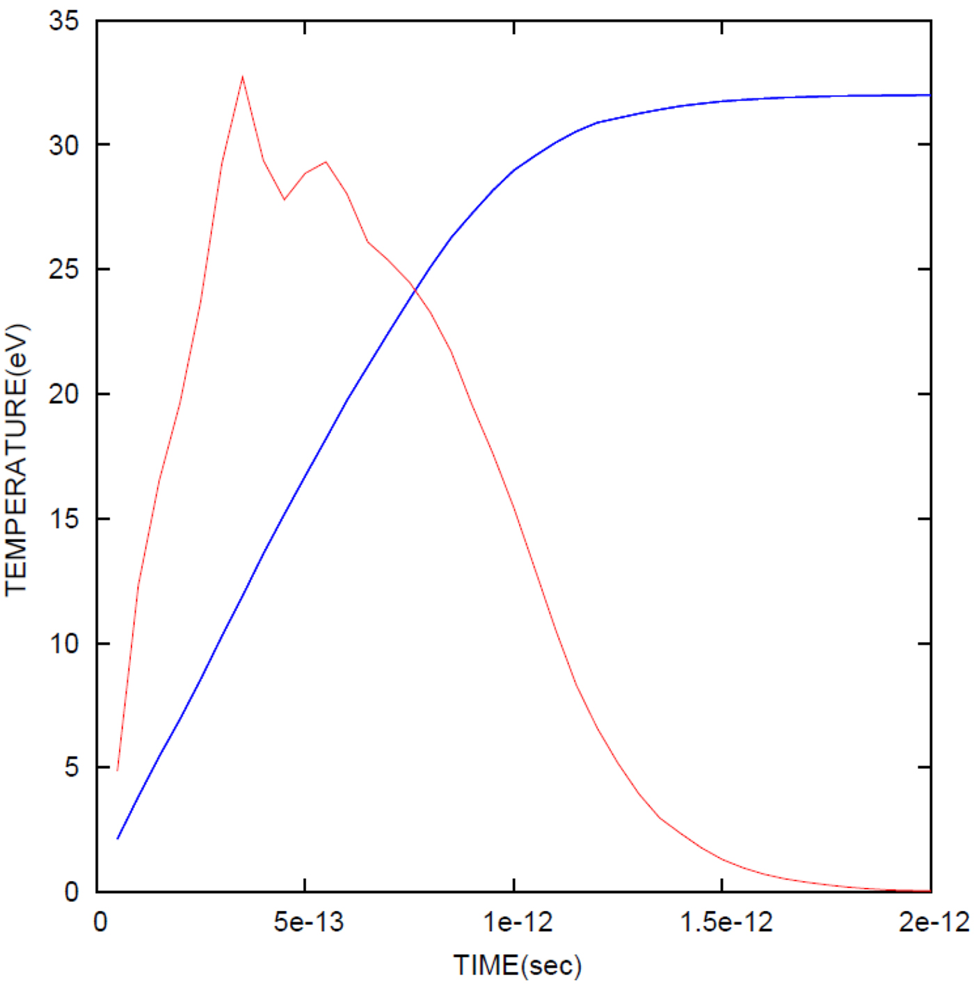
Fig. 8. Modeling of time-dependent temperature curve, in blue, where its asymptotic approach to the final temperature is observed. The other curve in brown is the temperature-dependent Kα pulse from previous graph, normalized to the temperature curve.
ACKNOWLEDGMENTS
We gratefully acknowledge the important contributions of Evgeny Stambulchik to this paper and also thank Eyal Kroupp for helpful discussions.
APPENDIX
TEMPORAL BEHAVIOR OF Kα RADIATION AND OF ENERGY DEPOSITION
We calculate here the temporal profile of Kα radiation looking from the laser side of the target, and at the inner 160 μm cylinder. We account for Kα production cross section as a function of energy (Patoary et al., Reference Patoary, Alfazuddin, Haque, Basak, Taulukder, Karim and Saha2008) as well as for the self-absorption. In Figure 7, we give the number of 160 μm cylinder counts as a function of time for the 330 fs primary beam as well as for the next six refluxing steps from the back and front of the target. The top curve is the sum of all seven steps. The emission time increases with each refluxing step. Additional refluxing steps, if they exist, will further broaden the curve, but their contribution decreases with increasing refluxing step. The calculated emission time hardly exceeds here 1.5 ps, whereas a very recent temporal measurement gives times of the order of 6 ps (Nilson et al., Reference Nilson, Davies, Theobald, Jaanimagi, Mileham, Jungquist, Stoeckl, Begishev, Solodov, Myatt, Zuegel, Sangster, Betti and Meyerhofer2012). However in that experiment, the Kα radiation was measured from the whole of the target (in their theoretical analysis, they assume that the electrons diffuse throughout the whole target eventually losing all their energy). Our calculation on the other hand, gives the pulse only from the inner 160 μm cylinder, from which region the electrons drift outward due to refluxing. It would therefore be of great interest to measure the time-dependent Kα pulse from the inner 160 μm cylinder and make comparisons with our modeling.
Equation (2) above, gives the connection between the average temperature, which is the measured temperature, T AV (also referred to above as T exp) to the final temperature, T FIN, for the assumption that target heating is due only to the fast electron energy deposition. The time-dependent Kα pulse, Kα(t) was derived as described in the previous paragraph and presented in Figure 7. In Figure 8, we also plot Kα(t) together with time-dependent temperature pulse, T e(t) which was calculated on the basis of the electron energy deposition with the inclusion of refluxing. The target temperature was obtained from the deposited energy and from the specific heat, the derivation of which is given in Section 2. The final temperature was set to 32 eV, by adjusting the absolute value of the energy deposition. Thus using Eq. (2), the connection between T AV and T FIN, was obtained and yielded, T AV = 0.6T FIN, using the data plotted in Figure 8. In so doing, we obtain the value of the main uncertainty in the calculation of the energy content of the target, where at the other extreme, T AV = T FIN; see text.