


INTRODUCTION
Reconstructing past vegetation composition from fossil pollen assemblages remains a central goal of palynology and paleoecology (Seddon et al., Reference Seddon, Mackay, Baker, Birks, Breman, Buck and Ellis2014) and serves many purposes. Reconstructions of prehistoric vegetation composition establish natural baselines, variability, and trajectories of forest composition before and during the emergence of intensive anthropogenic land use (Dawson et al., Reference Dawson, Cao, Chaput, Hopla, Li, Edwards and Fyfe2018). Such reconstructions enable the quantitative study of the biotic and abiotic drivers of forest dynamics at centennial to multimillennial time scales (Schoonmaker and Foster, Reference Schoonmaker and Foster1991). As ecological forecasting emerges as a distinct field of inquiry (Clark et al., Reference Clark, Carpenter, Barber, Collins, Dobson, Foley and Lodge2001; Dietze, Reference Dietze2017; Dietze et al., Reference Dietze, Fox, Beck-Johnson, Betancourt, Hooten, Jarnevich and Keitt2018), long-term vegetation reconstructions, accompanied by well-grounded estimates of uncertainty, offer empirical constraints on terrestrial ecosystem models of vegetation dynamics and the biogeochemical and biogeophysical interactions between the atmosphere and terrestrial biosphere (Bonan, Reference Bonan2008; Dawson et al., Reference Dawson, Paciorek, Goring, Jackson, McLachlan and Williams2019).
Reconstructing vegetation from fossil pollen is difficult due to the complexity of the relationship between vegetation composition and observed sedimentary pollen (e.g., Prentice, Reference Prentice1985). Relevant processes include intertaxon differences in pollen productivity and dispersal, spatial heterogeneity in forest composition at local to landscape scales, and the preservation and taphonomic modification of pollen assemblages during atmospheric transport and sedimentary deposition (Jackson, Reference Jackson and Traverse1994). To account for these complexities, pollen–vegetation models (PVMs) are used to infer past vegetation from fossil pollen and forest data. PVMs have progressed from more empirically based approaches (Parsons and Prentice, Reference Parsons and Prentice1981; Webb et al., Reference Webb, Howe, Bradshaw and Heide1981; Heide and Bradshaw, Reference Heide and Bradshaw1982; Jackson, Reference Jackson1990) to process-based models that quantify the complex processes that relate vegetation to pollen deposition by accounting for taxon-specific pollen production and dispersal (Prentice, Reference Prentice, Huntley and Webb1988; Sugita, Reference Sugita1994). The first process-based PVM to reach widespread adoption was the landscape reconstruction algorithm that includes the REVEALS and LOVE submodels (Sugita, Reference Sugita2007a, Reference Sugita2007b; Theuerkauf et al., Reference Theuerkauf, Couwenberg, Kuparinen and Liebscher2016), which is based on classical statistical inference. More recently, the Bayesian hierarchical PVM STEPPS has been developed (Paciorek and McLachlan, Reference Paciorek and McLachlan2009; Dawson et al., Reference Dawson, Paciorek, McLachlan, Goring, Williams and Jackson2016, 2019). Both models aim to describe the same processes, but they differ in several fundamental ways. To date, there has been no formal comparison of these models, their structures, or their predictions.
REVEALS (Sugita, Reference Sugita2007a) is widely used to estimate vegetation composition at regional to continental scales (e.g., Gaillard et al., Reference Gaillard, Sugita, Mazier, Trondman, Broström, Hickler and Kaplan2010; Trondman et al., Reference Trondman, Gaillard, Sugita, Bjorkman, Greisman, Hultberg, Lageras, Lindbladh and Mazier2016; Marquer et al., Reference Marquer, Gaillard, Sugita, Poska, Trondman, Mazier and Nielsen2017) and is a cornerstone of recent global initiatives such as LandCover6k (Dawson et al., Reference Dawson, Cao, Chaput, Hopla, Li, Edwards and Fyfe2018). REVEALS reconstructions typically involve the application of the model to networks of large lakes (>102 ha), based on the understanding that the regional-scale vegetation signal is stronger in larger pollen catchments (Sugita, Reference Sugita1994). REVEALS estimates the regional “background” pollen signal; its sister model, LOVE (Sugita, Reference Sugita2007b), then estimates local vegetation composition based on networks of smaller lakes and the regional background pollen signal. REVEALS models pollen deposition using a diffusion model that describes atmospheric transport of small particles originating from a ground-level point source (Sugita, Reference Sugita1994, Reference Sugita2007a). Taxon-specific atmospheric diffusion is mainly controlled by pollen fall speeds, which are a function of particulate size, mass, and shape, and is estimated based on grain measurements from still-air experimental settings or based on grain size and morphology (Jackson and Lyford, Reference Jackson and Lyford1999). Differential pollen productivity is represented by taxon-specific estimates of relative pollen productivity, estimated from sedimentary pollen and vegetation survey data (e.g., Calcote, Reference Calcote1995; Jackson and Kearsley, Reference Jackson and Kearsley1998; Nielsen, Reference Nielsen2004). Estimates of relative abundance of taxa and their uncertainties are based on classical statistical inference. REVEALS estimates are also influenced by depositional basin radius; the depositional basin radius determines the lower limit of the integral that specifies how far pollen has to disperse to reach the depositional site (typically assumed to be at the center of the basin). REVEALS estimates of regionally homogeneous vegetation composition are based on individual locations where pollen data are available and typically represent a region with a radius of 50–400 km. More recently, Pirzamanbein et al. (Reference Pirzamanbein, Lindstrom, Poska, Sugita, Trondman, Fyfe and Mazier2014, Reference Pirzamanbein, Lindstrom, Poska and Gaillard2018) have developed methods to estimate gridded vegetation composition from REVEALS-based vegetation reconstructions in a Bayesian Gaussian Markov random field framework.
STEPPS (Paciorek and McLachlan, Reference Paciorek and McLachlan2009; Dawson et al., Reference Dawson, Paciorek, McLachlan, Goring, Williams and Jackson2016, 2019) employs a process-based Bayesian hierarchical modeling framework to estimate the relative abundance of plant taxa in space (grid) and time using spatiotemporal networks of pollen records and a calibration vegetation composition data set. STEPPS consists of two components: (1) a calibration model and (2) a prediction model that relies on parameter estimates from the calibration model to reconstruct past vegetation. The calibration model characterizes the relationship between sedimentary pollen and vegetation and is used to estimate the taxon-specific parameters that describe production and dispersal processes. In the calibration model, at each depositional site, pollen sources are decomposed into two components, representing pollen from vegetation in the same grid cell versus nonlocal grid cells. We note that this decomposition into local and nonlocal components is similar to the landscape reconstruction algorithm decomposition into local and nonlocal components, although the latter specifies this division at the relevant source area of pollen, while for STEPPS this division is determined by the size of the focal grid cell. Dispersal is modeled using a specified dispersal kernel. Parameters are optimized so that the calibration model best explains observed pollen deposition at all sites simultaneously, given observed vegetation in the calibration domain and prior distributions of parameters.
After process parameter estimation using the STEPPS calibration model and spatial networks of pollen and vegetation data, the prediction model uses the pollen deposition model as specified in the calibration model, networks of fossil pollen data, and a spatiotemporally explicit framework to infer past vegetation composition for grid cells both with and without observed fossil pollen data. STEPPS estimates posterior spatiotemporal probabilities of vegetation composition, which represent the process and data uncertainty. These uncertainty estimates enable assessment of the precision of inferred changes of vegetation composition. In contrast to REVEALS, STEPPS has only been applied to two areas: a proof-of-concept demonstration in central New England, northeastern United States (NEUS; Paciorek and McLachlan, Reference Paciorek and McLachlan2009), and the upper midwestern United States (UMW; Dawson et al., Reference Dawson, Paciorek, McLachlan, Goring, Williams and Jackson2016, 2019). Hence the sensitivity of STEPPS parameter estimates and inference to choice of calibration region remains unclear.
Similarly, the effect of choice of PVM on vegetation reconstruction remains unclear, as there has been no systematic comparison between vegetation reconstructions obtained from REVEALS and STEPPS. While these two PVMs are both process-based and broadly similar in theoretical foundation, they exhibit important differences in model structure and parameter estimates that may result in differences in inferred vegetation. Key model differences include: (1) representation of pollen dispersal (differences among dispersal kernels and pollen fallspeeds), pollen dispersal distances and structural differences in whether local and regional pollen sources are distinguished; (2) model-specific taxon-specific estimates of pollen productivity; (3) differences in the treatment of spatiotemporal dependencies among sites; (4) methods for model calibration, including differences in spatial scale of vegetation considered for parameter estimation; and (5) spatial resolution of vegetation reconstructions.
In this study, we use REVEALS and STEPPS to reconstruct vegetation composition for a single time period: the pre–Euro-American settlement era for the NEUS. To do this, we use a network of pollen samples determined by expert elicitation to be from just before intensified land use associated with the Euro-American settlement era (i.e., from approximately 1620 to 1825). We first describe the data sources and PVMs in more detail. We then compare (1) REVEALS and STEPPS reconstructions to each other and to statistical estimates of forest composition (Paciorek et al., Reference Paciorek, Goring, Thurman, Cogbill, Williams, Mladenoff, Peters, Zhu and McLachlan2016) based on tree count data from the Township Proprietor Survey (Cogbill et al., Reference Cogbill, Burk and Motzkin2002; Thompson et al., Reference Thompson, Carpenter, Cogbill and Foster2013) and (2) parameter estimates used in REVEALS and STEPPS that characterize pollen dispersal and productivity. We also assess the sensitivity of STEPPS parameter estimates to the spatial extent of the calibration domain by evaluating the degree of similarity in these parameter estimates for the two studied regions.
DATA AND METHODS
Spatial and temporal domain
Spatially, this study encompasses the northeastern United States (NEUS), including Maine, New Hampshire, Vermont, Massachusetts, New York, Connecticut, Rhode Island, New Jersey, and Pennsylvania. This region has an area of 420,000 km2 and comprises four U.S. Forest Service ecoregions (Thompson et al., Reference Thompson, Carpenter, Cogbill and Foster2013): (1) Laurentian mixed forest province, (2) Adirondack–New England mixed forest–coniferous forest, (3) Eastern broadleaf forest, and (4) Central Appalachian broadleaf forest–coniferous forest. Elevation ranges from sea level to 1900 m above sea level.
In this work we focus on the pre–Euro-American settlement era for four reasons: (1) this time period predates major Euro-American land clearance in the 1700s and early 1800s (e.g., Hall et al., Reference Hall, Motzkin, Foster, Syfert and Burk2002; Russell, Reference Russell1983; Thompson et al., Reference Thompson, Carpenter, Cogbill and Foster2013); (2) vegetation composition data already have been digitized, bias corrected, and spatiotemporally modeled (Cogbill et al., Reference Cogbill, Burk and Motzkin2002; Thompson et al., Reference Thompson, Carpenter, Cogbill and Foster2013; Paciorek et al., Reference Paciorek, Goring, Thurman, Cogbill, Williams, Mladenoff, Peters, Zhu and McLachlan2016); (3) there is a regionally dense network of pollen records with samples from this time period (e.g., Oswald et al., Reference Oswald, Foster, Shuman, Doughty, Faison, Hall, Hansen, Lindbladh, Marroquin and Truebe2018); and (4) pollen samples from this era can be identified using biostratigraphic markers such as the increases in Ambrosia and Rumex abundances (e.g., Brugam, Reference Brugam1978).
Vegetation data
For the NEUS, forest composition data are available beginning in the seventeenth century, when trees were often used to mark property boundaries when granting land to Euro-American settlers. From these historical archives, Cogbill et al. (Reference Cogbill, Burk and Motzkin2002) have compiled data on forest composition during the settlement era for individual townships (Cogbill et al., Reference Cogbill, Burk and Motzkin2002; Thompson et al., Reference Thompson, Carpenter, Cogbill and Foster2013). These data, called the Town Proprietor Survey (TPS), extend from AD 1620 to AD 1825 (Thompson et al., Reference Thompson, Carpenter, Cogbill and Foster2013).
Recently, Paciorek et al. (Reference Paciorek, Goring, Thurman, Cogbill, Williams, Mladenoff, Peters, Zhu and McLachlan2016) developed a conditionally autoregressive model to estimate gridded vegetation composition for the Euro-American settlement era based on both the TPS (NEUS; Cogbill et al., Reference Cogbill, Burk and Motzkin2002;Thompson et al., Reference Thompson, Carpenter, Cogbill and Foster2013) and Public Land Survey (Ohio to Minnesota) data (Goring et al., Reference Goring, Williams, Mladenoff, Cogbill, Record, Paciorek, Jackson, Dietze and McLachlan2016). This work resulted in a spatially comprehensive ensemble of composition estimates, allowing the uncertainty of forest composition to be quantified. We use this gridded (8 km x 8 km) settlement-era forest composition (genus-level) product in this work.
We reconstruct forest composition for 13 tree taxa common in the NEUS: Fraxinus (ash), Fagus (beech), Betula (birch), Castanea (chestnut), Tsuga (hemlock), Carya (hickory), Acer (maple), Quercus (oak), Pinus (pine), Picea (spruce), Larix (larch, as only species L. laricina is native to eastern North America, this taxon is later on referred to as tamarack), other conifers (primarily of Abies [fir]), and other hardwoods (Alnus, Celtis, Corylus, Juglans, Magnolia, Moraceae, Morus, Nyssa, Ostrya/Carpinus, Platanus, Prunus, Rhamnus, Rhus, Salix, Sambucus, Shepherdia, Tilia). The choice of taxa to be reconstructed was primarily based on the abundance of taxa in the vegetation and pollen data, as well as their ecological importance (e.g., tamarack as the only deciduous conifer). Additionally, the taxonomic resolution possible depended on the taxonomic resolution of the vegetation data set produced by Paciorek et al. (Reference Paciorek, Goring, Thurman, Cogbill, Williams, Mladenoff, Peters, Zhu and McLachlan2016). For instance, Paciorek did not estimate gridded vegetation proportions of Alnus, which precluded modeling Alnus at the genus level using STEPPS.
The taxa reconstructed in the NEUS are not identical to the taxa reconstructed in the UMW. A comparison of parameter estimates for chestnut and hickory is therefore not possible.
Pollen data and identification of pre-settlement horizon
In this study, we use pollen records from the Neotoma Paleoecology Database (www.neotomadb.org [accessed 31 December 2017]; Williams et al., Reference Williams, Grimm, Blois, Charles, Davis, Goring and Graham2018) for the defined spatial and temporal domains and records contributed by individual authors (Supplementary Tables 1 and 2). In total, we gathered 187 pollen records from the NEUS, of which 161 have pollen samples from the late Holocene (here defined as having at least one sample between −70 BP and 4000 BP, using AD 1950 as “present”). The majority of these records came from Neotoma (126), 19 were from Oswald et al. (Reference Oswald, Foster, Shuman, Doughty, Faison, Hall, Hansen, Lindbladh, Marroquin and Truebe2018) and 7 from Paciorek and McLachlan (Reference Paciorek and McLachlan2009). We obtained additional data from Jackson (Reference Jackson1989), Whitehead and Jackson (Reference Whitehead and Jackson1990), Jackson and Whitehead (Reference Jackson and Whitehead1991), and LeBoeuf (Reference LeBoeuf2014). During analysis, most of these records were uploaded to Neotoma.
The time-transgressive nature of Euro-American settlement, uncertainties in radiometric dating, and the TPS make it difficult to identify pollen samples from the corresponding era based on the estimated age of sample. In lieu of this, for each pollen record, we used expert elicitation to identify the pollen samples representative of vegetation just before the Euro-American settlement era (e.g., Dawson et al., Reference Dawson, Paciorek, McLachlan, Goring, Williams and Jackson2016; Supplementary Table 1). Pollen stratigraphic plots of the most abundant northeastern arboreal taxa, as well as Rumex and Ambrosia (Foster et al., Reference Foster, Clayden, Orwig and Hall2002), were each assessed by three to four experts (drawn from an expert panel consisting of Robert K. Booth, SJG, WWO, JWW, and STJ). Experts were asked to indicate the most recent pollen sample representing largely undisturbed forests; they also indicated the certainty of their assessment on a three-point scale.
Only sites for which at maximum one expert expressed doubt about the existence of a settlement/pre-settlement boundary were included in the NEUS calibration data set. For sites included in the calibration data set, the expert-selected samples were sorted in ascending order with respect to depth. Given three expert determinations, we used the median depth as the depth of the settlement-era sample. For four-expert determinations, we used the median or in cases when the median was not an assigned depth, the second deepest sample depth was taken as depth of the settlement-era sample. For the 13 taxa considered, pollen identified at species or subspecies level were aggregated to genus level.
Pollen–vegetation models
Both PVMs compared here have been previously described in the literature: STEPPS (Paciorek and McLachlan, Reference Paciorek and McLachlan2009; Dawson et al., Reference Dawson, Paciorek, McLachlan, Goring, Williams and Jackson2016, 2019) and REVEALS (Sugita, Reference Sugita2007a). Here we describe key features of each model in some detail to provide a foundation for understanding observed similarities and differences between reconstructions and among reconstructions and observations. We also flag places where the methods followed here differ from those reported in previous papers.
STEPPS
STEPPS is a Bayesian hierarchical PVM used to estimate past vegetation composition from fossil pollen count data. In STEPPS, vegetation predictions based on observed pollen counts depend on (1) a calibration model that links gridded vegetation to pollen count data via a pollen dispersal and production process model and (2) a prediction model that uses calibration parameter estimates to infer latent gridded vegetation from fossil pollen counts for times and grid cells for which there are no vegetation data.
STEPPS calibration model
The calibration model describes the key processes that link pollen to vegetation, including taxon-specific pollen productivity and pollen dispersal. Parameters that specify these processes are estimated given observed gridded vegetation and a network of pollen samples from the same era. In STEPPS, pollen deposition at a site is divided into two components: pollen originating from the vegetation within the same grid cell (local) and pollen originating from other grid cells (nonlocal). The contribution of nonlocal vegetation (specified to be up to a maximum of 700 km from the depositional site) to the pollen record at a deposition site is a decreasing function of distance. In STEPPS, this distance dependence is represented using a dispersal kernel. Dawson et al. (Reference Dawson, Paciorek, McLachlan, Goring, Williams and Jackson2016) compared the Gaussian and (inverse) power-law families for both taxon-specific and single shared-across-taxa kernel models. Pollen productivity, proportion of local pollen deposition, and dispersal parameters are estimated using Bayesian inference; in other words, process parameter posterior estimates from the calibration model best explain observed pollen deposition given observed vegetation.
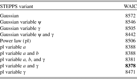
Mathematical descriptions of dispersal kernels and model priors are given in Dawson et al. (Reference Dawson, Paciorek, McLachlan, Goring, Williams and Jackson2016). Briefly, the Gaussian dispersal kernel depends on a single parameter ψ (characterizing the spread of the kernel), while the inverse power-law kernel depends on two parameters a and b (jointly characterizing the spread and mass in the tails). Following Dawson et al. (Reference Dawson, Paciorek, McLachlan, Goring, Williams and Jackson2016), we estimate parameters for two versions of the model: a version wherein parameters are constant across all taxa and a version wherein parameters vary among taxa. For the power-law kernel, b is allowed to vary among taxa if and only if a is also allowed to vary among taxa. The quality of candidate models is assessed using the Watanabe-Akaike information criterion (WAIC; Watanabe, Reference Watanabe2010; Table 1); this criterion is better suited to complex Bayesian hierarchical models, because it does not depend on the specific model parameterization.
Table 1. Watanabe-Akaike information criterion (WAIC, goodness-of-fit measure) for the calibration models for model variants. Lowest WAIC value is marked in bold.
Here we modify the priors used in the inverse power-law dispersal kernel in Dawson et al. (Reference Dawson, Paciorek, McLachlan, Goring, Williams and Jackson2016). Dawson et al. (Reference Dawson, Paciorek, McLachlan, Goring, Williams and Jackson2016) constrained the probability mass of a to values between 0 and 500 for the model employing a single shared dispersal kernel among taxa and log(a) to values between log(10−4) and log(500) when a was allowed to vary among taxa. In this work we constrain the probability mass of a and log(a) to maximum values of 1 and log(1), respectively, while the lower bound is kept unchanged. This stricter constraint was enforced because (1) the pollen network in the NEUS is less dense than in the UMW, resulting in less-constrained parameter estimates, and (2) values of a greater than 0.5 resulted in dispersal kernels that did not show decreasing dispersal as a function of distance from the pollen source.
STEPPS prediction model
The second component of STEPPS, the prediction model, describes vegetation composition as a spatial Gaussian process. For the gridded domain and for a single time interval, this process is multivariate normal (MVN). For taxon k,
 $$g_k\sim {\rm MVN[ }{\rm \mu }_k\comma \;{\rm \eta }_k{\rm exp}( -{\rm d}/{\rm \rho }_k) ] $$
where μk is the mean of the Gaussian process, and ηk and ρk determine the spatial dependencies among process values that are separated by distance d. The Gaussian process is then transformed into vegetation proportions via an additive log-ratio transformation:
 $$ r_k( s) = \displaystyle{{ {\rm exp} [ g_k (s)] } \over {\mathop \sum \nolimits_{k = 1}^K \; {\rm exp} [ g_k (s)] }}$$
where the superscript K is the total number of taxa, and s represents a specific grid cell.
This transformation ensures that the relative abundances of the taxa in the effective contributing vegetation sum to 1. This effective contributing vegetation is then used to simulate pollen deposition using the calibration model. Pollen counts Yi at a depositional site i are modeled as a Dirichlet multinomial, where
 $$Y_i\sim {\rm DM}( n_i\comma \;r_i^{{\rm pol}} ) $$
and ni is the number of pollen grains counted at site i and ri pol is a vector of taxon-specific concentration parameters with
 $$E(X_i) = \displaystyle{{r_i^{\,pol} } \over {\mathop \sum \nolimits r_i^{\,pol} }}$$
specifying the relative frequency X with which pollen from each taxon arrives at site i.
In the last step, we determine the probability of obtaining the observed pollen counts given simulated pollen deposition and number of pollen grains counted at each site, assuming that observed pollen follow a Dirichlet-multinomial distribution, which is an overdispersed multinomial distribution.
Conceptually, STEPPS is the combination of a statistical vegetation model (Gaussian process and subsequent sum-to-one constraint) and a pollen dispersal/deposition model (calibration model), with both models contributing to the overall posterior probability (agreement between simulated vegetation and spatial structure imposed and probability of obtaining observed pollen deposition as a function of simulated vegetation).
The dependencies in this model make it computationally demanding. As a result, it is not possible to estimate spatial dependence parameters and vegetation predictions simultaneously. We therefore first tested an empirical Bayes approach (Efron and Hastie, Reference Efron and Hastie2016) and estimated the parameters that describe the spatial dependence of vegetation, η and ρ, before estimating latent vegetation itself. Parameters of spatial dependence are estimated using a latent Gaussian process as in the full prediction model, but these latent Gaussian processes are linked to settlement-era tree count data (Cogbill et al., Reference Cogbill, Burk and Motzkin2002). Vegetation proportions are determined through a sum-to-one constraint and are then linked to tree count data with a multinomial model:
 $$V_j\sim {\rm multinom}( N_j\comma \;r_j) $$
where Vj is a vector of tree counts at location j, Nj is the total number of trees at location j, and rj is a vector of modeled vegetation proportions at location j.
However, the relatively low density of tree count data available in the TPS ultimately made it impossible to meaningfully estimate spatial dependence parameters. We therefore used parameters estimated for the UMW by Dawson et al. (Reference Dawson, Paciorek, McLachlan, Goring, Williams and Jackson2016) to model spatial dependence of vegetation, while using the NEUS calibration data to estimate pollen productivity and dispersal parameters.
STEPPS was implemented using the Stan statistical modeling software. The calibration model was implemented in Stan v. 2.17.1, while the prediction model was implemented in Stan v. 2.6.2. The prediction model was identical to the model implemented by Dawson et al. (Reference Dawson, Paciorek, McLachlan, Goring, Williams and Jackson2016) using analytical gradient evaluation allowing for parallel computation implemented using openMP (OpenMP Architecture Review Board, 2008).
REVEALS
REVEALS (Sugita, Reference Sugita2007a) is a PVM based on classical statistical inference. REVEALS assumes that the pollen signal produced by the regional vegetation around a large (>100 ha) depositional site will be fully mixed and homogenized during pollen transport, with no spatial structure persisting. Alternatively, REVEALS can employ networks of smaller lakes to estimate an average regional vegetation (e.g., Sugita et al., Reference Sugita, Parshall, Calcote and Walker2010). Its companion model, LOVE (Sugita, Reference Sugita2007b), is used to estimate local-scale vegetation composition given knowledge about the regional vegetation provided by REVEALS. Continental- to hemispheric-scale vegetation reconstructions typically rely on only REVEALS (Trondman et al., Reference Trondman, Gaillard, Mazier, Sugita, Fyfe, Nielsen and Twiddle2015; Marquer et al., Reference Marquer, Gaillard, Sugita, Poska, Trondman, Mazier and Nielsen2017). In these coarse-scale reconstructions, the prescribed radii of (inferred) regional vegetation producing a homogeneous pollen signal typically vary between 50 km (Trondman et al., Reference Trondman, Gaillard, Sugita, Bjorkman, Greisman, Hultberg, Lageras, Lindbladh and Mazier2016) and 400 km (Sugita, Reference Sugita2007a). REVEALS also assumes that all deposited pollen is sourced from within the prescribed regional radius.
Pollen dispersal/deposition within this homogenized vegetation is modeled as a function of vegetation composition based on a ground-level particulate dispersal model (Sutton, Reference Sutton1953). To estimate vegetation composition based on deposited pollen at a location, the pollen deposition model is solved for vegetation composition (Sugita, Reference Sugita2007a, Eq. 5). Pollen deposition is determined by two taxon-specific parameters: pollen productivity and a pollen dispersal deposition coefficient (K) that summarizes pollen dispersal and deposition into one coefficient. K in turn depends on a taxon-specific estimate of pollen fallspeed, a site-specific lake radius, and the prescribed maximum radius for regional pollen source area. Coefficient K also depends on several parameters describing atmospheric conditions: wind speed, vertical diffusion, and turbulence. These parameters are usually treated as constants but depend on atmospheric conditions (neutral or unstable). In this study, we assume neutral atmospheric conditions. This assumption is challenged by Jackson and Lyford (Reference Jackson and Lyford1999), who argue that most pollen are transported under unstable atmospheric conditions. Note that when REVEALS is used without LOVE, there is no explicit treatment of space in the reconstruction for each location (except for maximum distance of pollen dispersal influencing K).
Following standard practice (e.g., Trondman et al., Reference Trondman, Gaillard, Sugita, Bjorkman, Greisman, Hultberg, Lageras, Lindbladh and Mazier2016), we average REVEALS reconstructions from sites within a 1° by 1° grid cell; this averaging reduces the site-level signal.
For REVEALS, we use pollen productivity estimates (PPEs) from the NEUS (Jackson and Kearsley, Reference Jackson and Kearsley1998), UMW (Bradshaw and Webb, Reference Bradshaw and Webb1985; Calcote, Reference Calcote1995), Quebec, Canada (Chaput and Gajewski, Reference Chaput and Gajewski2018), and Alaska, USA (Hopla, E., and Edwards, M., personal communication, 2017; Table 2). These PPEs do not include a PPE for American chestnut (Castanea dentata), the dominant species of chestnut in the study area, which precluded modeling of REVEALS-based chestnut abundances. We model the other hardwood and other conifer taxa using PPEs and pollen fallspeeds of the most important genera, Alnus (alder) and Abies (fir). For PPEs lacking uncertainty estimates, we assume that the ratio PPE/standard error of PPE is constant for a taxon among studies. We restandardize PPEs using oak as the reference taxon. This standardization requires an adjustment of both the mean PPE as well as the standard error. The standard error of PPEs is determined by
 $$s_{{\rm taxon}}^2 = ( {\rm PP}{\rm E}_{{\rm taxon}}/{\rm PP}{\rm E}_{{\rm ref}}) ^2\ast [ ( s_{{\rm PPEtaxon}}/{\rm PP}{\rm E}_{{\rm taxon}}) ^2 + ( s_{{\rm PPEref}}/{\rm PP}{\rm E}_{{\rm ref}}) ^2] $$
Table 2. Pollen productivity estimates and uncertainties used for REVEALS.

We use published pollen fallspeeds from several sources (Bodmer, Reference Bodmer1922; Dyakowska, Reference Dyakowska1936; Durham, Reference Durham1946; Eisenhut, Reference Eisenhut1961). Lake sizes are available for 90 sites (Supplementary Table 1). We draw lake sizes for the remaining 20 sites from a truncated normal distribution defined by the median of the observed sizes as mean and the square of the interquartile range of the observed sizes as variance.
To implement the REVEALS model, we use the R REVEALS package DISQOVER developed by Theuerkauf et al. (Reference Theuerkauf, Couwenberg, Kuparinen and Liebscher2016). Estimates of uncertainty associated with vegetation reconstructions differ between disqover and the original method implemented by Sugita (Reference Sugita2007a). In DISQOVER (Theuerkauf et al., Reference Theuerkauf, Couwenberg, Kuparinen and Liebscher2016), pollen count uncertainty is modeled using proportions of observed pollen as a probability vector to simulate pollen counts from a multinomial distribution. We note that this approach affects reconstructed vegetation in pollen samples with low counts of taxa with very low pollen dispersal–deposition coefficients (Abies, Larix). PPE uncertainty in disqover is also accounted for by drawing PPE values from a normal distribution specified by the mean and standard error of PPE values.
Comparison of STEPPS and REVEALS: reconstructions and parameter estimates
We compare settlement-era vegetation reconstructions estimated using STEPPS and REVEALS to (1) each other and (2) the Paciorek et al. (Reference Paciorek, Goring, Thurman, Cogbill, Williams, Mladenoff, Peters, Zhu and McLachlan2016) settlement-era vegetation data set. These comparisons assess the difference in relative abundance of taxa for each grid cell for individual taxa and at the community level. Community-level differences were quantified using grid cell–wise squared chord distance (SCD; i.e., squared Euclidean distances of square-root-transformed composition vectors). To compare REVEALS-based estimates to the Paciorek et al. (Reference Paciorek, Goring, Thurman, Cogbill, Williams, Mladenoff, Peters, Zhu and McLachlan2016) data set, we assume that REVEALS estimates represent homogeneous vegetation within a 1° by 1° grid cell. As for STEPPS, reconstructed vegetation is assumed to be homogeneous within an 8 km by 8 km grid cell. For both models, reconstructed vegetation is compared with the forest composition data for each 8 km by 8 km grid cell falling within the larger PVM-specific grid cell.
To simplify and summarize the dissimilarity comparisons, we define three forest types based on qualitative assessment of dominant taxa (oak: proportions of oak > 0.3, beech: proportions of beech > 0.3, spruce: proportions of spruce > 0.4). We estimate dissimilarities (SCDs) within and among forest types. This comparison allows us to determine whether differences in relative abundance in the models and data are primarily within or among forest types (e.g., Gavin et al., Reference Gavin, Oswald, Wahl and Williams2003).
STEPPS and REVEALS are based on similar theoretical principles but differ in implementation. Differences between STEPPS and REVEALS reconstructions are potentially due to: (1) differences in taxon-specific estimates of relative pollen productivity; (2) differences in dispersal models, determined by dispersal kernels and fallspeeds; and (3) differences in the treatment of spatial dependence.
Both STEPPS and REVEALS use taxon-specific pollen scaling parameters/PPEs to weight pollen counts/proportions. To compare the inferred STEPPS pollen scaling parameters to the predefined productivity values used in REVEALS, we standardize the STEPPS estimates using oak as a reference taxon. We assess whether the predefined REVEALS productivity values fall within the 95% credible interval of the STEPPS productivity estimates.
Pollen dispersal distance and pollen source area are more difficult to directly compare. For both STEPPS and REVEALS, it is in principle possible to quantify the radius within which a certain percentage of pollen originates (i.e., source area; Prentice, Reference Prentice, Huntley and Webb1988) or is deposited (i.e., capture radius). For STEPPS, which currently implements dispersal as an isotropic process and does not account for variability in lake size, the source area and capture radius are identical. In REVEALS, however, lake radius is used to define a minimum dispersal distance. The taxon-specific dispersal function is integrated with a lower integration boundary defined by the lake radius and the upper integration boundary defined by the maximum dispersal distance. The result of this integration is the pollen dispersal–deposition coefficient (K). We compare the K coefficients and pollen fallspeeds from REVEALS to the 70% capture radii calculated using the dispersal kernel from STEPPS. We expect that the REVEALS K coefficients and fallspeeds should be proportional and inversely proportional, respectively, to the STEPPS capture radii.
RESULTS
Site selection, expert elicitation, and comparison of pollen and vegetation data
For 86 of the 161 pollen records, all experts agreed on the existence of a settlement-era horizon. For 34 pollen records, only one expert expressed doubt about the existence of a settlement-era horizon. For the remaining 41 records, at least two experts expressed doubt about the existence of a settlement-era signal, so these 41 records were discarded from all subsequent analyses. Of the 120 pollen records that were determined to contain a settlement signal, 9 were from locations outside the vegetation data extent, making them unsuitable for inclusion in the calibration data set. These extraneous locations included coastal islands near Massachusetts and Maine, and Lake Ontario. An additional site lacked the taxonomic resolution needed for our analysis and was removed (i.e., no taxonomic discrimination below the level of Pinaceae). Two sites from Neotoma that lacked age constraints but showed a clear settlement-era signal were added to the NEUS calibration data set. More complete site information is given in Supplementary Table 1.
Pie maps of settlement-era pollen assemblages and vegetation show spatially consistent patterns of dominant taxa (Fig. 1). Oak pollen and trees are most abundant in southeastern New England, with a northern limit close to the northern border of Massachusetts. Spruce and birch pollen and trees are most abundant in the northeast, while beech pollen and trees are found in New York, northeastern Pennsylvania, and Massachusetts. Hemlock pollen and trees are found in western New York, northeastern Pennsylvania, and southern Maine. These broad-scale congruences provide the basis for further efforts to quantitatively calibrate and predict forest composition from fossil pollen data.

Figure 1. Pie maps depicting proportions of tree genera of pollen (a) and settlement-era vegetation (b) based on spatially modeled Township Proprietor Survey data (Paciorek et al., Reference Paciorek, Goring, Thurman, Cogbill, Williams, Mladenoff, Peters, Zhu and McLachlan2016). CT, Connecticut; LO, Lake Ontario; MA, Massachusetts; ME, Maine; NH, New Hampshire; NJ, New Jersey; NY, New York; PA, Pennsylvania; RI, Rhode Island; VT, Vermont. Blue rectangle in inset map indicates study area. (For interpretation of the references to color in this figure legend, the reader is referred to the web version of this article.)
STEPPS calibration
STEPPS calibration model parameters were estimated for each of the 10 variants of the dispersal kernels tested using Stan with 250 warm-up and 2000 sampling iterations. In all cases, convergence metric Rhat was smaller than 1.005, providing evidence to suggest sampler convergence (Gelman et al., Reference Gelman, Carlin, Stern, Dunson, Vehtari and Rubin2013).
Of the 10 model variants considered, the power-law dispersal kernel models with variable a and γ (percentage of pollen deposited locally) outperformed other dispersal models (based on WAIC; Table 1). For most taxa, observed and modeled pollen deposition are in agreement; that is, the relationship between observed and modeled pollen deposition is linear, with a slope not significantly different from 1 (Supplementary Fig. 1, significant correlations and r > 0.6). However, for pine, other hardwoods, ash, and tamarack, the relationship between observed and modeled pollen deposition is weaker (r < 0.5; Supplementary Fig. 1); for chestnut, modeled pollen deposition is systematically lower than observed pollen deposition. This assessment suggests that the STEPPS calibration model accounts for the key processes that link pollen and vegetation and that, for most taxa, the information in the available data (sedimentary pollen and vegetation) is sufficient to estimate the parameters that describe these processes.
Comparison of STEPPS and REVEALS
Predicted vegetation
The vegetation predictions from both STEPPS and REVEALS capture the broad-scale observed vegetation patterns in the NEUS, but there are also systematic discrepancies among the two reconstructions and observed vegetation for some taxa and regions (Fig. 2, Supplementary Fig. 2; see Supplementary Fig. 3 for STEPPS uncertainties).

Figure 2. (color online) Heat maps of settlement-era vegetation. Median estimates of relative abundance for beech, hemlock, oak, and spruce from a spatially modeled form of the Township Proprietor Survey (TPS) data (left, Paciorek et al., Reference Paciorek, Goring, Thurman, Cogbill, Williams, Mladenoff, Peters, Zhu and McLachlan2016), STEPPS (center), and REVEALS (right).
Vegetation patterns predicted by STEPPS consistent with observed patterns include abundant oak in the southeast, beech in the northwest, spruce in northern Maine and the Adirondacks, and hemlock in a central area ranging from northern Pennsylvania to southern Maine. Vegetation predictions for western Pennsylvania show less concordance with observations; STEPPS overpredicts hemlock, likely due to the lack of pollen records from this region. However, for many taxa, observed versus predicted taxon abundances at depositional sites show systematic departures from the one-to-one line, indicating over- or underprediction by STEPPS (Fig. 3, Supplementary Fig. 4). In particular, STEPPS predictions do not sufficiently reproduce the distributions of pine, other conifers, and other hardwoods (Supplementary Figs. 2 and 4).

Figure 3. Comparison of fractional abundances from spatially modeled Township Proprietor Survey (TPS) data (Paciorek et al., Reference Paciorek, Goring, Thurman, Cogbill, Williams, Mladenoff, Peters, Zhu and McLachlan2016) and STEPPS and REVEALS for four representative taxa: beech, hemlock, oak, and spruce. All axes are expressed as fractional abundances relative to a sum consisting of all tree taxa considered here. For gridded datasets points are drawn from grid cells containing pollen sites.
Similar to STEPPS, REVEALS predicts many of the observed vegetation patterns, particularly the patterns of hemlock and beech (Fig. 2). However, REVEALS generally overpredicts other conifers (primarily fir) and maple and underpredicts oak (Figs. 2 and 3, Supplementary Figs. 2 and 4).
There are substantial differences between predictions of relative abundances from STEPPS and REVEALS for individual sites (Fig. 3, Supplementary Fig. 4). These differences reflect the over- and underpredictions noted in the comparisons to observed general vegetation patterns (Figs. 2 and 3).
At a community level, dissimilarities between observed and STEPPS-predicted vegetation composition show distinct spatial patterns (Fig. 4), with relatively low dissimilarities in the southeastern NEUS, southern Maine, eastern New York, and Vermont. Higher dissimilarities occur in western Pennsylvania, west central New York, and along the oak–beech ecotone. Dissimilarities between STEPPS reconstructions and observed vegetation (Paciorek et al., Reference Paciorek, Goring, Thurman, Cogbill, Williams, Mladenoff, Peters, Zhu and McLachlan2016) are slightly lower than dissimilarities between REVEALS reconstructions and observed vegetation data, with mean SCDs of 0.33 and 0.39, respectively (for full summary statistics, see Supplementary Table 3). The difference between the model versus data SCDs is statistically significant (Wilcoxon signed-rank test, P < 0.05), although the difference (effect size) is very small (ΔSCD = 0.06). When comparing within-forest-type and among-forest-type dissimilarities, the boundary between the two categories is at an SCD of about 0.4 (Supplementary Fig. 5), meaning that most dissimilarities between observed and reconstructed vegetation belong to the within-forest-type category.

Figure 4. Community-level comparison of STEPPS predictions for the settlement era to the spatially modeled Township Proprietor Survey (TPS) data at 8 km by 8 km grid. Comparisons are expressed as squared chord distance (SCD) between STEPPS predictions of vegetation composition and the spatially modeled TPS inferences from Paciorek et al. (Reference Paciorek, Goring, Thurman, Cogbill, Williams, Mladenoff, Peters, Zhu and McLachlan2016). High SCDs (reds) indicate larger discrepancies between the original TPS inferences and STEPPS predictions. (For interpretation of the references to color in this figure legend, the reader is referred to the web version of this article.)
Pollen productivity and dispersal
Standardized PPEs used in REVEALS are only weakly correlated to the STEPPS estimated productivity values (ρ = 0.51, P = 0.09; Fig. 5a). STEPPS pollen scaling parameters were consistently higher than PPEs in the literature. Additionally, literature-based PPEs do not fall within the 95% credible interval of STEPPS-based pollen scaling parameter estimates, except for the reference taxon oak having a standardized PPE of 1 for both models. Both show pine as an above-average pollen producer. However, the STEPPS PPE for birch is high (four times that of oak), whereas the literature-based PPE for birch is less than the literature-based PPE for oak. Oak has the second-highest PPE value for REVEALS, but the eighth-highest value in the STEPPS pollen scaling parameter.

Figure 5. (color online) Comparison between STEPPS and REVEALS parameter estimates relating to pollen productivity and dispersal. (a) Comparison of prescribed pollen productivity estimates (PPEs) in REVEALS to STEPPS estimates of the phi scaling parameter that represents intertaxonomic differences in pollen productivity. (b) Comparison of prescribed pollen fallspeeds in REVEALS to STEPPS estimates of 70% pollen capture radii (with the expectation that fallspeed should be inversely related to capture radius). (c) Comparison of STEPPS capture radii to REVEALS pollen dispersal deposition coefficients (K) for a lake radius of 550 m. (d) Comparison among K values for lake radii of 5.5, 55, 550, and 5500 m. The radius of regional vegetation in the REVEALS simulations is set to 100 km. Uncertainties of STEPPS-based parameter estimates are shown in Fig. 6 (Phi) and Table 3 (capture radii).

Figure 6. Comparison of pollen productivity estimates (Φ) estimated by STEPPS for independent calibrations in the upper midwestern United States (UMW; red) and northeastern United States (NEUS; cyan). These simulations use the variable power-law pollen dispersal kernel. Whiskers indicate credible intervals based on posterior distributions of parameter estimates. (For interpretation of the references to color in this figure legend, the reader is referred to the web version of this article.)
Table 3. Radii (km) from a pollen source needed to capture 50%, 70%, and 90% of the dispersed pollen for the Gaussian and power-law models with lowest Watanabe-Akaike information criterion. Median capture radii are indicated along with 2.5% and 97.5% quantiles of the distribution of capture radii.

There is also a lack of agreement between the pollen fallspeeds used in REVEALS to capture radii estimated using STEPPS (ρ = −0.34, P = 0.28; Fig. 5b). Some individual taxa show expected relationships; for example, there is good agreement for hemlock, with a high pollen fallspeed (REVEALS prescribed) and a short capture radius (STEPPS inferred). Conversely, the relationships for oak do not agree, with low pollen fallspeeds (REVEALS) yet the shortest capture radius (STEPPS).
As with pollen fallspeeds, pollen dispersal–deposition coefficients (K) estimated by REVEALS are only weakly related to STEPPS capture radii (Fig. 5c). Pearson's correlation coefficients for taxon-specific correlations between K and STEPPS radii increase with increasing lake size in REVEALS but are not significant (P > 0.05). REVEALS produces three clusters of pollen dispersal deposition coefficients (Fig. 5c): (1) hemlock, other conifers, and tamarack, which have low values; (2) beech, spruce, and maple, which have intermediate values; and (3) oak, hickory, ash, alder (other hardwoods), pine, and birch, which have high values. Conversely, no clustering is apparent in the STEPPS capture radii.
Note that changing the lake radius in REVEALS has only a minor effect on reconstructed vegetation. For the 110 samples considered in this study, changing the lake radius from 5.5 m to 5500 m results in SCDs among vegetation reconstructions between 0.02 and 0.2 with quartiles of 0.08, 0.09, and 0.11.
STEPPS calibration comparisons: UMW and NEUS
Estimates of STEPPS pollen scaling parameters compare favorably between the NEUS and UMW, although several taxa have larger capture radii for the NEUS than the UMW (Figs. 6 and 7). Ordering of pollen scaling parameters is largely similar between regions (Fig. 6), and credible intervals (95%) of pollen scaling parameters overlap for 6 out of 11 taxa. Pollen productivity credible intervals are generally wider for the NEUS than for the UMW. In particular, the credible intervals are widest for NEUS pine and tamarack.

Figure 7. Comparison of pollen dispersal kernels estimated by STEPPS for independent calibrations in the upper midwestern United States (UMW; black) and northeastern United States (NEUS; red). Cumulative proportion of pollen deposited as a function of distance. Solid lines depict power-law kernels (PLK) and dashed lines depict Gaussian kernels (GK). (For interpretation of the references to color in this figure legend, the reader is referred to the web version of this article.)
Pollen capture radii (Table 3) are generally larger for the NEUS than for the UMW (e.g., hemlock, birch, beech, pine) due to differences in modeled dispersal kernels and proportions of pollen deposited locally (Fig. 7, Supplementary Fig. 6), indicating that STEPPS estimates larger source areas for the NEUS. Pine has the largest differences in capture radii, with 70% pollen capture radii of 512 km (NEUS) and 260 km (UMW) for the variable power-law dispersal kernel. Power-law dispersal kernels and capture radii estimated for oak and spruce for the UMW and NEUS are indistinguishable (Fig. 7, Table 3).
DISCUSSION
Overview
This paper presents the first formal comparisons of predictions and parameter estimates of the two PVMs STEPPS and REVEALS; it also presents the first sensitivity test of STEPPS parameter estimates to the spatial domain used for calibration. The comparison of these PVMs shows both a general congruence of predictions between models and with observed vegetation (Fig. 2), but also highlights important differences between PVMs and their structures, parameter estimates, and predictions. Comparisons of STEPPS parameter estimates for the UMW (Dawson et al., Reference Dawson, Paciorek, McLachlan, Goring, Williams and Jackson2016) and NEUS (this study) are generally consistent, suggesting that for geographically separated but floristically similar regions, and at the scales considered here, STEPPS parameter estimates are mostly unaffected by choice of calibration region. However, estimated parameter uncertainties are larger for the NEUS than for the UMW. Overall, these findings suggest that STEPPS is successfully translating similarities between spatial patterns of observed pollen and observed vegetation (Fig. 1) into similarities between predicted vegetation and observed vegetation (Fig. 2). However, the STEPPS-based vegetation reconstructions tend to be less accurate and precise for the NEUS than for the UMW. Here, we focus on diagnosing discrepancies between reconstructions and between observations and reconstructions to provide insight into PVM structure and behavior and to identify avenues for future work.
Reconstructed versus observed vegetation
Data availability clearly affects STEPPS accuracy: STEPPS-based vegetation reconstructions agree well with the gridded TPS vegetation data for the most abundant taxa (beech, birch, oak, and spruce) in regions with sufficient spatial coverage by sampled pollen records, while vegetation reconstructions for less abundant taxa or regions with limited spatial coverage by or absent from the sampled pollen records generally show less agreement (Figs. 2 and 4). For example, for hemlock, STEPPS predictions generally match observations in most regions well (Fig. 2), except in northern Pennsylvania and central New York, where pollen records are sparse.
Sparse observations affect STEPPS predictions, because only locations for which there are pollen data constrain the predicted spatial vegetation patterns (i.e., contribute to the posterior probability through the likelihood function of the pollen process model component). Edge effects tend to amplify challenges associated with data sparsity, for example, in northern Maine (Fig. 2). The vegetation data for northern Maine indicate that other conifers (fir) are widespread throughout the state in substantial amounts; however, there are few pollen depositional sites within Maine, which precludes meaningful estimation of the proportion of pollen deposited locally. Additionally, northern Maine is receiving pollen from vegetation outside the domain, while STEPPS assumes that all pollen deposited at any location is sourced from vegetation within the study domain.
For individual taxa, discrepancies among vegetation reconstructions and observations usually can be traced back to particular parameter estimates. Oak is underrepresented by REVEALS, because oak has a high predefined PPE (second highest) and also a low pollen fallspeed (high K), resulting in low reconstructed/predicted vegetation abundances. Conversely, oak is well represented by STEPPS both in terms of abundance and spatial domain. Maple and other conifers have low PPEs in REVEALS, resulting in high relative abundances (see Eq. 5 in Sugita, Reference Sugita2007a). Maple and other conifers also have low estimated productivity in STEPPS (Fig. 5), but in this case both are underpredicted (Supplementary Fig. 2). This discrepancy is probably caused by differences between dispersal models in STEPPS and REVEALS (Fig. 5b and d). For instance, in REVEALS, maple has a relatively high pollen fallspeed (and thereby low K), resulting in high estimates of maple abundance, while STEPPS estimates a relatively large capture radius indicative of either good pollen dispersal or a poorly constrained dispersal kernel. Finally, STEPPS and REVEALS treat pine as a prolific pollen producer with good dispersal abilities (i.e., low pollen fallspeed for REVEALS). This results in underestimation of pine abundances by both PVMs.
Note that considering taxa individually can only partly explain discrepancies among vegetation reconstructions and observations. For both PVMs, the fractional abundances reconstructed for individual taxa depend on pollen counts and parameters of all taxa, creating an interdependence among all taxon-level reconstructions.
REVEALS versus STEPPS: model structure and parameter estimates
Because we use the same settlement-era pollen assemblages for both STEPPS and REVEALS, differences in reconstructed vegetation are attributable to differences in model structure and parameter estimates.
Although both PVMs are process-based models, the PVMs fundamentally differ in their treatment of space. STEPPS explicitly models vegetation in space (Fig. 2), whereas REVEALS only accounts for space through the dependence of the pollen dispersal deposition coefficient (K) on an assumed maximum distance of pollen dispersal (Sugita, Reference Sugita2007a). The maximum distance of pollen dispersal is prescribed by the user and usually varies between 50 km (Trondmann et al., Reference Trondman, Gaillard, Sugita, Bjorkman, Greisman, Hultberg, Lageras, Lindbladh and Mazier2016) and 400 km (Sugita, Reference Sugita2007a; see Methods section).
To make gridded predictions, STEPPS considers all depositional sites simultaneously in calibration and models pollen deposition at all these sites simultaneously in prediction, whereas REVEALS makes predictions for a single depositional site (and surrounding area) at a time. It is then possible to average REVEALS-based reconstructions for sites from the same grid cell (e.g., Trondman et al., Reference Trondman, Gaillard, Sugita, Bjorkman, Greisman, Hultberg, Lageras, Lindbladh and Mazier2016; this study) or to obtain gridded reconstructions using methods described in Pirzamanbein et al. (Reference Pirzamanbein, Lindstrom, Poska and Gaillard2018).
The differences in taxon-level parameter values between STEPPS and REVEALS are also striking. Estimates of pollen productivity using STEPPS and REVEALS are comparable with a few notable exceptions (Fig. 5a). Most notably, pollen productivities of birch and oak differ strongly.
According to the scientific understanding of pollen dispersal, pollen fallspeeds should strongly control pollen dispersal distances (Prentice, 1985; Sugita, Reference Sugita2007a). In this study, however, there is no clear relation between capture radii simulated by STEPPS and the pollen fallspeeds and K coefficients used in REVEALS (Fig. 5b–d; see also Dawson et al., Reference Dawson, Paciorek, McLachlan, Goring, Williams and Jackson2016). The discrepancy of STEPPS and REVEALS dispersal parameters might be explained by challenges in measuring pollen fallspeeds (Jackson and Lyford, Reference Jackson and Lyford1999). Jackson and Lyford (Reference Jackson and Lyford1999) also argue that atmospheric conditions have a stronger influence on K than pollen fallspeeds.
Generally, differences in model parameters (pollen productivity and dispersal parameters) can be caused by the fact that model parameters are optimized for a certain model structure and a specific set of pollen and vegetation observations. For instance, STEPPS is calibrated on settlement-era pollen and vegetation data, whereas PPEs used for REVEALS are based on modern pollen assemblages and vegetation data drawn from a variety of systems and scales (e.g., Jackson and Kearsley, Reference Jackson and Kearsley1998; Chaput and Gajewski, Reference Chaput and Gajewski2018). Differences in pollen–vegetation relationships between pre-settlement and modern periods (Paciorek and McLachlan, Reference Paciorek and McLachlan2008; Kujawa et al., Reference Kujawa, Goring, Dawson, Booth, Grimm, Hotchkiss, Jackson, Lynch., McLachlan, St. Jacques, Umbanhower and Williams2016) might explain some differences in parameters and vegetation reconstructions. A more comprehensive comparison of STEPPS and REVEALS would require calibration of both models using the same observed pollen and vegetation data, which was not possible in this study, because the TPS data do not have sufficient spatial resolution to meaningfully use extended R-value models traditionally used to estimate pollen productivities.
The effects of optimizing model parameters for a specific model structure are illustrated by the 10 variants of STEPPS compared by Dawson et al. (Reference Dawson, Paciorek, McLachlan, Goring, Williams and Jackson2016). Each model variant resulted in different estimates of the pollen scaling parameter (equivalent to PPEs; see Dawson et al., Reference Dawson, Paciorek, McLachlan, Goring, Williams and Jackson2016, Fig. 5) as all parameters are optimized for a given model structure (taxon-specific parameters or global parameters, Gaussian or inverse power-law dispersal kernel). Additionally, changing the maximum pollen dispersal distance (results shown for 700 km) changes parameter estimates.
Theuerkauf et al. (Reference Theuerkauf, Kuparinen and Joosten2012) found that PPEs are sensitive to choice of pollen dispersal model (equivalent to changing the weighting of the observed vegetation or changing the physics of pollen dispersal), the size of the lakes used for estimation (small vs. medium size), and the estimation method (extended R-value model vs. simulation approaches). PPEs used in REVEALS are typically obtained using extended R-value models (Parsons and Prentice, Reference Parsons and Prentice1981; Prentice and Parsons, Reference Prentice and Parsons1983; Prentice and Webb, Reference Prentice and Webb1986; Sugita, Reference Sugita1994). Vegetation surrounding a depositional site is weighted to approximate the distance-dependent scaling imposed by pollen dispersal when determining PPEs (e.g., Jackson and Kearsley, Reference Jackson and Kearsley1998). PPEs considered in the present study consisted of published values determined using inverse distance weighting, inverse squared distance weighting, and the Prentice-Sugita model (Jackson and Kearsley, Reference Jackson and Kearsley1998; Chaput and Gajewski, Reference Chaput and Gajewski2018). When observed vegetation is weighted using the Prentice-Sugita model, weighting depends on pollen fallspeeds and parameters describing atmospheric conditions and is equivalent to the weighting applied by REVEALS. Additionally, using extended R-value models to estimate PPEs creates interdependencies among PPEs; changing the weighting applied to observed vegetation of one taxon will result in changes to PPEs of all taxa (e.g., Theuerkauf et al., Reference Theuerkauf, Kuparinen and Joosten2012).
The areal extent of vegetation considered for estimating pollen productivity varies widely among studies and models, from a radius of 100 m around moss polsters and hollows (Calcote, Reference Calcote1995; Jackson and Kearsley, Reference Jackson and Kearsley1998) to a radius of 30 km around larger lakes (>9 ha) (Bradshaw and Webb, Reference Bradshaw and Webb1985). More formally, the relevant source area of pollen (RSAP) is defined as the distance beyond which including additional vegetation does not improve fit (as measured by the relevant likelihood function) between weighted vegetation and observed pollen deposition (Sugita, Reference Sugita1994). This does not mean that no pollen is originating from distances further than the RSAP; rather, pollen originating from larger distances can be modeled as a homogeneous signal. Early simulation studies (e.g., Sugita, Reference Sugita1994) typically find RSAP < 1 km. Chaput and Gajewski (Reference Chaput and Gajewski2018) found an RSAP of 1.6 km for sites in Quebec, Hjelle and Sugita (Reference Hjelle and Sugita2011) found an RSAP of between 0.9 km and 1.1 km for western Norway, and Theuerkauf et al. (Reference Theuerkauf, Kuparinen and Joosten2012) found an RSAP between 5 km and 12 km for northeastern Germany.
In contrast, STEPPS uses gridded vegetation data at 8 km by 8 km resolution and allows for pollen transport up to 700 km. PPEs used for REVEALS are therefore based on local vegetation around a depositional site, whereas pollen scaling parameters used for STEPPS are based on regional and supraregional-scale vegetation, while STEPPS does not resolve processes at the subgrid scale. Ultimately, REVEALS resolves processes that STEPPS summarizes as local pollen deposition, whereas STEPPS resolves processes of pollen dispersal that REVEALS treats as a homogeneous regional pollen signal.
For instance, REVEALS accounts for site-specific lake sizes, with large lakes expected to carry a regional vegetation signal, whereas small lakes are more indicative of local vegetation (Sugita, Reference Sugita2007a, Reference Sugita2007b). For pollen assemblages used in this study, lake sizes only have moderate effects on vegetation reconstructions, with SCDs indicating that the differences in reconstructions obtained from varying lake size are only in the within-forest-type category (see “Results” section). Still, considering lake size in STEPPS might account for some of the heterogeneity of the pollen observations.
General agreement of REVEALS- and STEPPS-based vegetation reconstructions highlights the value of both reconstruction techniques. STEPPS offers the advantages of being able to generate gridded reconstructions and estimate their associated uncertainty.
This uncertainty is estimated based on a large number of posterior draws (consisting of estimates of proportional abundances of each taxon for each grid point). These draws from the posterior distribution can be used to calculate pairwise differences in the proportional abundance of a taxon at two sites (grid points), allowing for the quantification of systematic differences in proportional abundances even with high uncertainties of mean abundances (e.g., Paciorek and McLachlan, Reference Paciorek and McLachlan2009). From a statistical viewpoint, the uncertainties obtained using STEPPS and REVEALS are not directly comparable. Uncertainties estimated for REVEALS are uncertainties of the mean of reconstructed vegetation (confidence intervals), whereas STEPPS-based uncertainties are uncertainties of single point predictions that are assumed to represent a vegetation in a grid cell whose size is specified by the model (predictive intervals).
However, this advantage comes at the cost of requiring vegetation observations to calibrate the vegetation model. STEPPS is a spatiotemporal Bayesian hierarchical model that accounts for the complex spatiotemporal dependence structure of the vegetation and is therefore computationally expensive. This expense additionally limits the applicability of STEPPS. REVEALS is more straightforward to apply in practice, which in turn results in broader applicability. For instance, region- or continent-specific estimates of pollen productivity and pollen fallspeeds have been shown to be sufficient to develop REVEALS-based reconstructions. Recently, methods have been developed to obtain gridded reconstructions of land cover using REVEALS-based spatially homogeneous estimates (Pirzamanbein et al., Reference Pirzamanbein, Lindstrom, Poska, Sugita, Trondman, Fyfe and Mazier2014, 2018). These estimates are based on integrated nested Laplace approximations (Rue et al., Reference Rue, Martino and Chopin2009) and are therefore computationally inexpensive. Additionally, Theuerkauf et al. (Reference Theuerkauf, Kuparinen and Joosten2012, Reference Theuerkauf, Couwenberg, Kuparinen and Liebscher2016) extended REVEALS using different pollen dispersal functions, for instance, Lagrangian dispersal models (Kuparinen et al., Reference Kuparinen, Markkanen, Riikonen and Vesala2007).
STEPPS NEUS and UMW: comparison of parameter estimates
Estimates of pollen productivity and dispersal parameters are similar between the two studied regions (Figs. 6 and 7), but parameter uncertainties are larger for the NEUS. The general concordance between STEPPS results for both regions (Figs. 6 and 7) suggests that mean estimates of taxonomic parameters in STEPPS are not highly sensitive to the domain of calibration and data set size for floristically similar regions; however, uncertainty does seem sensitive to region and/or size of the calibration data set.
Reconstructing vegetation for the NEUS is a priori more challenging than for the UMW for several reasons. First, the data sources used for settlement-era vegetation reconstructions differ considerably between the two regions. In the UMW, gridded (0.8 km by 0.8 km) tree counts from the Public Land Survey were first aggregated to an 8 km by 8 km grid (Goring et al., Reference Goring, Williams, Mladenoff, Cogbill, Record, Paciorek, Jackson, Dietze and McLachlan2016) and used to obtain statistical estimates of vegetation composition (Paciorek et al., Reference Paciorek, Goring, Thurman, Cogbill, Williams, Mladenoff, Peters, Zhu and McLachlan2016). For the NEUS, tree counts are available only at the township level and were preferentially selected to mark property boundaries (Cogbill et al., Reference Cogbill, Burk and Motzkin2002; Thompson et al., Reference Thompson, Carpenter, Cogbill and Foster2013). Hence, tree surveys in the TPS were less systematic and have fewer counts than the Public Land Survey, with 860,000 trees in the midwestern domain and 420,000 trees in the northeastern domain (Paciorek et al., Reference Paciorek, Goring, Thurman, Cogbill, Williams, Mladenoff, Peters, Zhu and McLachlan2016). The TPS data contain known biases, given that they were based on unsystematic and nonrandom selection by landowners of trees for marking property boundaries (Whitney and DeCant, Reference Whitney, DeCant, Egan and Howell2001), yet they have also been shown to accurately capture regional-scale vegetation patterns (Cogbill et al., Reference Cogbill, Burk and Motzkin2002; Thompson et al., Reference Thompson, Carpenter, Cogbill and Foster2013). These differences in vegetation sampling between the Public Land Survey and TPS increase uncertainty in statistical estimates of vegetation composition in the NEUS (Paciorek et al., Reference Paciorek, Goring, Thurman, Cogbill, Williams, Mladenoff, Peters, Zhu and McLachlan2016).
The density of pollen sites is also lower in the NEUS. While the areal size of the two domains is similar, predictions are based on 220 UMW sites (Dawson et al., Reference Dawson, Paciorek, McLachlan, Goring, Williams and Jackson2016) versus 110 NEUS sites (Fig. 1, Supplementary Table 1). The two regions also differ with respect to topography and physiography. In the UMW, the main vegetational gradients correlate to latitudinal variations in temperature and longitudinal variations in precipitation (Curtis, Reference Curtis1959) with modest topographic relief. In contrast, the NEUS is topographically complex, and variability in elevation and terrain leads to increased local-scale variability in forest composition. Hence, NEUS vegetation tends to be more spatially heterogeneous at scales of 101–102 km than UMW vegetation. This increased spatial heterogeneity makes it more difficult to accurately predict vegetation at locations without pollen observations, at least in the absence of additional predictors in the model.
Regional shape, position, and edge effects may also affect STEPPS reconstructions in the two regions studied. The UMW domain used by Dawson et al. (Reference Dawson, Paciorek, McLachlan, Goring, Williams and Jackson2016) (Minnesota, Wisconsin, Upper Michigan Peninsula) is roughly rectangular and bordered by prairie to the west and Lake Michigan to the east. This reduces the amount of arboreal pollen originating from outside the reconstructed domain. In contrast, the NEUS extends from southwest to northeast and is bordered by forested areas to the west and northwest. These extraregional sources of pollen likely confound STEPPS modeling for the NEUS.
Pollen dispersal distances are generally greater in the NEUS than in the UMW (Table 3, Supplementary Fig. 6). This may be caused by the more variable topography of the NEUS and by stronger turbulence caused by the more variable topography. Stronger turbulence has been shown to result in transport of pollen grains over greater distances (Jackson and Lyford, Reference Jackson and Lyford1999). Alternatively, the increased dispersal distances in the NEUS may result from lower correspondence between vegetation and pollen data, for example, in places where the pollen data indicate a taxon is present that is absent in the vegetation of the corresponding “local” grid cell. This might explain consistently lower proportions of pollen deposited locally (i.e., lower values of the γ parameter) in the NEUS than the UMW (Supplementary Fig. S6). This would mean that more pollen is modeled to originate from regional and extraregional sources, resulting in greater dispersal distances.
Two taxa—pine and tamarack—are difficult to model using existing data and modeling approaches in the NEUS. Generally, mismatches between local vegetation and pollen data as found for pine and tamarack (Fig. 1) result in (1) decreased estimates of local pollen deposition (e.g., for tamarack, large differences in the local deposition parameter between the UMW and NEUS; Supplementary Fig. 4), and (2) inflated estimates of pollen productivity or dispersibility (e.g., pine). In the TPS data (Paciorek et al., Reference Paciorek, Goring, Thurman, Cogbill, Williams, Mladenoff, Peters, Zhu and McLachlan2016), pine trees are present from central Pennsylvania and southern New Jersey through eastern New York, northern Connecticut, Massachusetts, western Vermont, the southern half of New Hampshire, and southern Maine (Fig. 1), while depositional sites in central Maine and the Adirondacks have the highest pollen percentages. TPS surveys likely missed some local pine stands that were important sources for depositional sites with high pine pollen abundances but apparently no nearby pine trees. Places with high local abundances of pine in the vegetation data set but low pine pollen abundances in the sediment are more puzzling, as pine is a prolific pollen producer (e.g., Bradshaw and Webb, Reference Bradshaw and Webb1985; Calcote, Reference Calcote1995; Dawson et al., Reference Dawson, Paciorek, McLachlan, Goring, Williams and Jackson2016), and complicate estimation of local pine pollen deposition. The poorly constrained NEUS pine dispersal kernels show little resemblance to pine dispersal kernels estimated for the UMW (Dawson et al., Reference Dawson, Paciorek, McLachlan, Goring, Williams and Jackson2016).
Tamarack is modeled poorly by STEPPS in both studied areas (Dawson et al., Reference Dawson, Paciorek, McLachlan, Goring, Williams and Jackson2016). Low abundances of tamarack pollen are both observed and expected due to the low pollen productivity and high pollen fallspeed of tamarack (Niklas, Reference Niklas1984; Dawson et al., Reference Dawson, Paciorek, McLachlan, Goring, Williams and Jackson2016; Fig. 5a). Paleoecological interpretation of tamarack is also complicated by its common occurrence in mires, making it difficult to differentiate pollen sourced from a few nearby local individuals versus a more widespread regional presence. Additionally, in this study, there are no pollen sites in locations where the settlement-era forest composition data set indicates tamarack presence, further complicating parameter estimation. The poor performance of REVEALS and STEPPS with respect to tamarack is unfortunate, given that tamarack is one of the few representatives of the deciduous conifer plant functional type. However, achieving accurate pollen-based inferences of past tamarack distributions may well be an intractable challenge for any PVM.
Future research opportunities
There are multiple pathways to improving past vegetation reconstructions and reducing uncertainties, with possibilities including additional data and model refinements. Pollen records available for this study are not distributed evenly in space. While there is a high density of records in southern New England, records are sparse in western Pennsylvania, central New York, Vermont, and northern Maine. Having more pollen samples representing the settlement era from these areas would probably improve calibration of tree taxa abundant in these areas and further constrain predictions of settlement-era vegetation.
Running STEPPS is currently computationally expensive and precludes application of STEPPS both at finer spatial scales and to larger regions. Implementing a more computationally tractable spatial model would allow modeling of pollen dispersal and deposition at scales finer than the 8 km by 8 km spatial resolution used in this work. The advantage of being able to estimate dispersal and deposition processes at finer scales is that it would allow for finer-scaled predictions, potentially allowing for a more robust inference about vegetation heterogeneity. However, the ability to more finely resolve these processes and predictions depends inherently on the resolution of the calibration vegetation data set and the density of pollen samples. We also note the interest in reconstructing vegetation in mountainous landscapes. The plausibility of using STEPPS in these regions depends on understanding the nature of pollen dispersal and deposition in these regions—dispersal is likely not isometric, resulting in the need for asymmetric and spatially varying dispersal kernels. The application of STEPPS to these high-relief mountainous areas would probably require explicitly accounting for elevation, perhaps as an environmental covariate for ecological similarity among grid cells (e.g., Fyfe et al., Reference Fyfe, Woodbridge and Roberts2015).
While REVEALS has been widely used to reconstruct relative abundance of both arboreal and nonarboreal vegetation types, to date STEPPS has only been used to reconstruct forest composition (arboreal taxa). For both REVEALS and STEPPS, the limitations to making accurate inference of nonarboreal vegetation types arise from the calibration data. For REVEALS, while PPEs are available for some arboreal types, there are many taxa for which they have yet to be developed. For STEPPS, existing calibration data sets rely on land survey data, which are exclusively arboreal taxa. For both models, the motivation to include nonarboreal taxa is to increase the usefulness of pollen-based land cover reconstructions for ecosystem and carbon cycle modelers (e.g., Dietze et al., Reference Dietze, Fox, Beck-Johnson, Betancourt, Hooten, Jarnevich and Keitt2018). In both cases, more developed calibration data sets would allow for inference about plant functional types, including grasslands and cultivated grains.
Paciorek and McLachlan (Reference Paciorek and McLachlan2008) calibrated an earlier version of STEPPS using settlement-era pollen and vegetation data and modern pollen and vegetation data from southern New England. They found significant differences in pollen scaling parameters of individual taxa, while dispersal characteristics (for a Gaussian dispersal kernel) remained unchanged. Extending such analyses to the entire NEUS and UMW would further test the temporal stability of and explore the effects of anthropogenic influences on pollen–vegetation relationships.
Simulation studies (e.g., Sugita, Reference Sugita1994) would allow testing of the accuracy and precision of STEPPS-based vegetation reconstructions as a function of data density, data distribution, and noise inherent in the data.
REVEALS is a more mature pollen vegetation model than STEPPS and has been applied and tested more extensively. Methodological work mainly focuses on the effects of pollen dispersal models (e.g., Sutton model and Lagrangian models; Theuerkauf et al., Reference Theuerkauf, Kuparinen and Joosten2012) and use of parameters describing atmospheric conditions (turbulent vs. stable) on estimates of pollen productivity and vegetation reconstructions. Research is also carried out in the field of parameter estimation with comparisons of different estimation methods such as extended R-value models and methods based on iterative approaches (e.g., Theuerkauf et al., Reference Theuerkauf, Kuparinen and Joosten2012; Fang et al., Reference Fang, Ma and Bunting2019). In its current form, REVEALS does not treat pollen records as time series and assumes that pollen assemblages within a sediment core are independent, nor does it account for temporal persistence of forest composition. REVEALS has mainly been employed to reconstruct vegetation composition in midlatitudes, and initiatives are underway to test and apply REVEALS in areas with vegetation fundamentally different from midlatitude vegetation, such as the tropics.
Finally, as pollen–vegetation modeling matures as a field, there will be an increasing number and variety of PVMs. As in other fields (e.g., Taylor et al., Reference Taylor, Stouffer and Meehl2012), formal model intercomparison projects with more comprehensive comparisons among PVMs would further our understanding of the reasons for differences among vegetation reconstructions; some pollen-based land cover reconstruction work has been done toward this goal (Roberts et al., Reference Roberts, Fyfe, Woodbridge, Gaillard, Davis, Kaplan and Marquer2018). In a first step, PVMs should be calibrated using the same pollen and vegetation data, eliminating differences among vegetation reconstructions caused by different calibration targets and regions. The comparison between STEPPS-based, spatial reconstructions and results of the spatial model introduced by Pirzamanbein et al. (Reference Pirzamanbein, Lindstrom, Poska and Gaillard2018) is also outstanding. Further application and refinement of STEPPS and REVEALS (spatial model and pollen dispersal functions) will improve our knowledge of past vegetation and land cover. This knowledge is crucial to understand interactions between past land cover changes and past regional climate (Gaillard et al., Reference Gaillard, Sugita, Mazier, Trondman, Broström, Hickler and Kaplan2010).
CONCLUSIONS
As the field of pollen–vegetation modeling matures, multiple process-based PVMs are now emerging, each with its variants, but the differences in structure and behavior among PVMs and variants have been less well understood. Here we show that both STEPPS and REVEALS are able to reconstruct general vegetation patterns observed during the Euro-American settlement era. STEPPS integrates a calibration and prediction model to produce fully spatial reconstructions, albeit with reduced accuracy in areas lacking pollen records. REVEALS reconstructions (without further spatial modeling) consist of estimates of homogeneous regional-scale vegetation assumed around a depositional location. The REVEALS and STEPPS reconstructions differ fairly substantially for some taxa, however, these differences can be traced to differences in pollen dispersal and productivity. In data-dense regions, STEPPS closely follows the data; however, in places where data are lacking, predictions tend to be poorly constrained and potentially inaccurate.
With this study, STEPPS has been successfully used to reconstruct settlement-era vegetation for two large areas, the UMW (Dawson et al., Reference Dawson, Paciorek, McLachlan, Goring, Williams and Jackson2016) and the NEUS. Modeled uncertainties tend to be higher in the NEUS, due to interregional differences in data density and tree survey data, topographic complexity, and proximity of extraregional sources of arboreal pollen.
ACKNOWLEDGMENTS
This work is a contribution to the Paleoecological Observation Network (PalEON) project, supported by the National Science Foundation (144-PRJ76IG, DEB-1241868, DEB-1241874, DEB-1241851) and National Science Foundation grants DEB-0620443, DEB-0815036, DEB-1146207, and DEB-1237491. This work also contributes to the PAGES LandCover6k working group. We thank Robert K. Booth for making pollen data from Bloomingdale Bog available. We thank the University of Notre Dame Center for Research Computing for providing access to resources and support. We also thank Jody Peters for assistance in team coordination. We thank associate editor Terri Lacourse and two anonymous reviewers for comments that improved the quality of this article. Code is available at: https://github.com/mtrachs/QR_STEPPS_REVEALS_NEUS.
SUPPLEMENTARY MATERIAL
The supplementary material for this article can be found at https://doi.org/10.1017/qua.2019.81.


