NOMENCLATURE

α

angle-of-attack

δ _ij

Kronecker delta

$a_{n} $

curve fit constants for the c _p equation

e

internal energy

q

dynamic pressure, 1/2ρV ²

$C_{i} $

mass fraction

C _p

pressure coefficient, (p−p _∞)/q _∞

c _p

specific heat at constant pressure

c _v

specific heat at constant volume

$D_{i} $

molecular diffusion constant

$he$

static enthalpy

h

Plank’s constant

$h_{{\rm d}} $

dissociation enthalpy per unit mass of air in the external flow

$h_{i} $

dissociation energy per unit mass

k

Boltzmann’s constant

$k_{{{\rm th}}} $

thermal conductivity constant

L

model reference length

$L_{{\rm e}} $

Lewis number

ρ

fluid density

P

pressure

R

gas constant

R _B

base radius

R _N

nose radius

S

distance from nose

T

temperature

x _i

co-ordinates (x ₁ =x, x ₂ =y, x ₃ =z)

u _i

velocity vector

V

velocity magnitude

E

total energy per unit volume

τ _ij

viscous stress tensor

ε

emissivity constant (≈1)

σ

Boltzmann constant

μ

dynamic viscosity

q

heat flux

$q_{{{\rm ref}}} $

heat flux at the stagnation point using Fay–Riddell method

R_e

Reynolds number

Pr

Prandtl number

M

Mach number

() _i

mass injection boundary conditions

()_e

edge of the boundary layer

( )_∞

freestream conditions

$()_{{{\rm out}}} $

boundary outflow conditions

( ) _t

turbulent quantity

$()_{{\rm w}} $

wall conditions

$$()_{{{\rm oe}}} $$

stagnation condition at the edge of the boundary layer

2.0 COMPUTATIONAL METHODOLOGY

It would be appropriate to provide some comments on the computational algorithm used for the present work. The conservative form of the compressible Reynolds-Averaged Navier–Stokes equations in index form is given as follows:

(1) $${{\partial {\rm \rrho }} \over {\partial t}}{\plus}{\partial \over {\partial x_{i} }}\left[ {{\rm \rrho }u_{i} } \right]{\equals}0$$

(2) $${\partial \over {\partial t}}\left( {{\rm \rrho }u_{i} } \right){\plus}{\partial \over {\partial x_{j} }}\left[ {{\rm \rrho }u_{i} u_{j} {\plus}p\rdelta _{{ij}} {\minus}\left( {1{\plus}{{\rmu _{t} } \over \rmu }} \right)\rtau _{{ij}} } \right]{\equals}0$$

(3) $${\partial \over {\partial t}}\left( {{\rm \rrho }E} \right){\plus}{\partial \over {\partial x_{j} }}\left[ {{\rm \rrho }u_{j} E{\plus}u_{j} p{\minus}\left( {1{\plus}{{{\rm \rmu }_{t} } \over {\rm \rmu }}} \right){u}_{i} {\rm \rtau }_{{ij}} {\minus}\left( {c_{p} {{\rm \rmu } \over {{\rm Pr}}}{\plus}c_{p} {{{\rm \rmu }_{t} } \over {{\rm Pr}_{t} }}} \right){{\partial T} \over {\partial x_{j} }}} \right]{\equals}0$$

ρ in these equations refers to the density, p the pressure and T is the temperature. E is the total energy and u is the velocity vector in tensor format. τ_ij is the viscous stress tensor which may be written as

(4) $${\rm \rtau }_{{ij}} {\equals}{\rm \rmu }\left( {{{\partial u_{i} } \over {\partial x_{j} }}{\plus}{{\partial u_{j} } \over {\partial x_{i} }}{\minus}{2 \over 3}{{\partial u_{k} } \over {\partial x_{k} }}\rdelta _{{ij}} } \right)$$

The Spalart–Almaras one-equation turbulence model is used to compute turbulent viscosity coefficient (μ _t ) for most of the present computations. The Wilcox two equations k–ω model demanding increased computational time was tried in a few cases without noting any improvements in results. The Sutherland law is implemented to compute the laminar viscosity coefficient ( $\rmu $ ). Since the flows computed involve hypersonic Mach number, the choice of the Prandtl number is selected to suite the Mach number whereas the use of specific heat and the specific heat ratio c _p/c _v (γ) in the algorithm for one species gas must also respect the high Mach number flow conditions subject to the relations⁽ Reference Grundmann ^{13 ,} Reference Gordon and McBride ^{14 )}:

(5) $$\eqalignno{ & c_{\rm v} \left( T \right){\equals}R\left( {{5 \over 2}{\plus}{{\left( {{{h{\rm v}} \over {kT}}^{2} } \right)e^{{{\raise0.7ex\hbox{${h\rm v}$} \!\mathord{\left/ {\vphantom {{h{\rm v}} {kT}}}\right.\kern-\nulldelimiterspace}\!\lower0.7ex\hbox{${kT}$}}}} } \over {\left( {e^{{{{h{\rm v}} \over {kT}}}} {\minus}1} \right)^{2} }}} \right),\quad c_{p} \left( T \right){\minus}c_{\rm v} \left( T \right){\equals}R \cr & {{c_{p} (T)} \over R}{\equals}\mathop{\sum}\limits_{n{\equals}0}^{n{\equals}4} {a_{n} T^{n} } $$

where T is the temperature, R is the real gas constant, h is Planck’s constant, v is the fundamental vibrational frequency and k is Boltzman’s constant and where $a_{n} $ are curve-fit constants.

Above Navier–Stokes equations are the first cast into curvilinear co-ordinate scheme following the Vinokur transformation⁽ Reference Vinokur ^{15 )} method. The numerical algorithm used to solve the Navier–Stokes equations is an implicit factorization finite difference scheme which is described at length by Beam and Warming⁽ Reference Beam and Warming ^{16 )}. Local time linearisation is applied to the non-linear terms and, following Pulliam and Chausee⁽ Reference Pulliam and Chaussee ^{17 )}, an approximate factorisation scheme is applied to the resulting matrices which factorizes the operator itself resulting in efficient matrix equations with narrow bandwidth. This results in block tridiagonal matrices which are easy to solve. The spatial derivatives can thus be approximated using second-order central differences. Explicit and implicit artificial dissipation terms are added to achieve nonlinear stability. A spatially variable time step is used to accelerate convergence to steady-state solutions.

The input flow conditions (ρ, ρu _i , e) for the outflow surface must be evaluated from the jet mass, momentum and static pressure conditions at the exit boundary. If the jet mass flow rate ( $\rrho u$ ) momentum ( $\rrho u^{2} )$ and jet static pressure ( $p_{{{\rm out}}} $ ) are known, as indeed was the case in Ref. Reference Nowak20, then ${\rrho \over {\rrho _{\infty} }}$ and ${{\rrho u} \over {\rrho _{\infty} u_{\infty} }}$ as well as the energy terms can be evaluated. These conditions are then treated like a new ‘slip’ condition which remains fixed during the flow-applied run. The algorithm iterates between the successive grid planes near the exit control boundary until the desired flow conditions are matched at the exit boundary as the convergence criterion is reached. For the corresponding solid surface run this surface would understandably carry a no-slip boundary. Alternatively, an outflow static pressure may be affixed at the control boundary to match the ultimate outflow conditions. The outflow pressure ( $p_{{{\rm out}}} $ ) and the corresponding Mach number ( $M_{{{\rm out}}} $ ) must be evaluated with respect to the pressure and the Mach number at the edge of the boundary layer. The boundary layer edge conditions may be obtained from a prior no outflow run. Other flow conditions for the algorithm may be evaluated as follows:

(6) $$\eqalignno{ & {{p_{{{\rm out}}} } \over {p_{e} }}{\equals}\left[ {{{1{\plus}{{\rgamma {\minus}1} \over 2}M_{e}^{2} } \over {1{\plus}{{\rgamma {\minus}1} \over 2}M_{{{\rm out}}}^{2} }}} \right]^{{{\rgamma \over {\rgamma {\minus}1}}}} ,\quad u_{{{\rm out}}} {\equals}M_{{{\rm out}}} \surd\left\{ {{{\rgamma p_{{{\rm out}}} } \over {\rrho _{{{\rm out}}} }}} \right\} \cr & \ e_{{{\rm out}}} {\equals}{{p_{{{\rm out}}} } \over {\rrho _{{{\rm out}}} (\rgamma {\minus}1)}}{\plus}{{u_{{{\rm out}}}^{2} } \over 2} \cr & he_{{{\rm out}}} {\equals}e_{{{\rm out}}} {\plus}{{p_{{{\rm out}}} } \over {\rrho _{{{\rm out}}} }} $$

Heat transfer was also computed for the three models investigated in this paper. The heat transfer in a hypersonic flow field which consists of dissociated gases is given by the equation:

(7) $$\dot{q}_{w} {\equals}k_{{th}} \left( {{{\partial T} \over {\partial y}}} \right)_{\!\!w} {\plus}\left( {\sum \rrho D_{i} h_{i} {{\partial C_{i} } \over {\partial y}}} \right)_{\!\!w}$$

where k _th is the thermal conductivity constant for the gas, $h_{i} $ is the dissociation energy per unit mass of atomic products, $D_{i} $ is the molecular diffusion constant of the ith-component of the mixture and $C_{i} $ refers to the mass fraction. For the present analysis only, the first term in equation⁽ Reference Glass, Dilley and Kelly ^{7 )} was recovered directly from the computed flow field. The diffusion terms which can be significant at high temperatures and other radiative heat from excited atoms and molecules in the shock layer or even catalytic effects from chemical reactions are not addressed in this analysis. Following the experiment, the reference point heat transfer value $\dot{q}_{w} {{_{\rm Ref}}} $ was obtained from Fay–Riddell equation⁽ Reference Fay and Riddell ^{18 )}:

(8) $$\dot{q}_{{\rm w}} {\equals}{{0.763} \over {\left( {{\rm Pr}_{{\rm w}} } \right)^{{0.6}} }}\rrho _{{\rm e}} u_{{\rm e}} ^{{0.4}} \rrho _{{\rm w}} u_{{\rm w}} ^{{0.1}} \left[ {h_{{\rm o}} _{_{\rm e}} {\minus}h_{{\rm w}} } \right]\left[ {1{\plus}\left( {L_{{\rm e}} ^{{0.52}} {\minus}1} \right){{h_{{\rm d}} } \over {h_{{\rm o}} _{_{\rm e}} }}} \right]\left[ {\left( {{{{\rm d}u_{{\rm e}} } \over {{\rm d}x}}} \right)_{t} } \right]^{{0.5}} $$

w and e refer to the wall and boundary layer edge conditions, $h_{{\rm o}} $ is the total enthalpy condition and $h_{{\rm d}} $ is the dissociation enthalpy per unit mass of air in the external flow. The Prandtl number ${\rm Pr}_{{\rm w}} $ value was 0.9 and the Lewis number $L_{{\rm e}} $ was assumed to be 1. The last term $\left( {{{{\rm d}u_{{\rm e}} } \over {{\rm d}x}}} \right)_{t} $ , in front of the blunt nose at the stagnation point t can be simply recovered from the relationship:

(9) $$\left( {{{{\rm d}u_{{\rm e}} } \over {{\rm d}x}}} \right)_{\!\!\!t} {\equals}{1 \over R}\sqrt {{{p_{{\rm e}} {\minus}p_{\infty} } \over {\rrho _{\infty} }}} $$

3.0 COMPUTATIONS

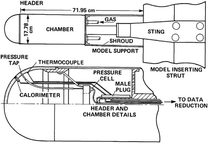
Navier–Stokes computations were performed on a number of hypersonic configurations. First validations were performed for the models used in actual wind tunnel experiments and, subsequently, more realistic hypersonic configurations were examined to see if the computations performed satisfactorily. The first of these is a cylindrical configuration supporting a hemispherical tip. The configuration shown in Fig. 1 was tested by Kaattari⁽ Reference Kaatari ^{19 )} at M=7.32 in the Reynolds number range 0.6×10⁶–5.2×10⁶. In the experiment, an externally supplied internal pressure of the model was balanced against the flow field external pressure to obtain the required mass flow rate through the porous frontal area. The mass flow rate profile was calculated in arbitrary units using a relationship of the form, $\dot{m}{\equals}cA(P_{{{\rm in}}}^{2} {\minus}P_{{{\rm ex}}}^{2} )$ , where c is a conductance constant at the point location, A is the sniffer tube area and P _in and P _ex refer to the chamber and external pressures. It is understood that the internal pressure is varied to obtain the non-constant velocity profile at the exit. The instrumentation is shown in Fig. 1. A complex flow profile was thus obtained at the leading edge. In the present computations, there were no means to vary the internal pressure against the external varying pressure field at the nose. A simplified constant exit velocity was applied to match a nominal mass flow rate of about ρu/ρ_∞ u _∞=0.027 used in the experiment. From this viewpoint, the exit outflow condition does not match exactly between simulation and the experiment.

Figure 1 Model support and flow control mechanism, Kaattari⁽ Reference Nowak ^{20 )}.

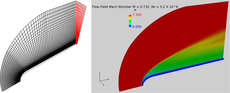
The CFD-based simulation of the above experiment was carried out at M=7.32 and unit Reynold s number 5.2×10⁶. The 3D mesh representing a 15° slice of the model used to simulate the flow is shown in Fig. 2. The Mach number-based flow field is also shown on the right-hand side of Fig. 2. The y+ value in all the models examined here was kept within a nominal value of 1. For more complex shapes discussed later, the y+ distribution around the surface is duly provided. A meticulous grid sensitivity study was carried out for each case discussed here. For brevity, these grid sensitivity results are not shown included here.

Figure 2 3D mesh of a 15° sliced cylindrical model with a helispherical nose, 90×100×15 (left). The computed Mach number field (right).

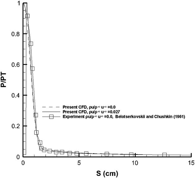
The computed pressure distribution for the solid surfaced model and the one supporting a flow ejection at the blunt hemispherical nose are shown in Fig. 3. The computed pressure agrees quite well with the measured pressure distribution. Note the low-pressure value at the stagnation region when the blowing is applied. Indeed owing to these low pressures at the stagnation region it would not be practical to apply the blowing across the entire region lest the aerodynamics performance is adversely affected. In the present case, therefore, the mass flow rate was applied to about 10% of the surface area adjacent to the stagnation region rather than the complete surface flow ejection profile used in the experiment.

Figure 3 Pressure distribution comparison for the hemispherically tipped cylindrical model.

Kaattari⁽ Reference Kaatari ^{19 )} explicitly states that the heat transfer performance of the model would be profoundly affected by the presence of the transition regime on the model surface, without actually defining the location or the extent of the transition region. The present computations were performed assuming fully turbulent flow without accounting for the transition effects. It should also be stated that the present method relies on holding the flow rates on the surface constant near the stagnation region rather than controlling the exact profile of the flow rates as depicted in the experiment. In a numerical simulation, it would be quite impractical to manually match the precise blowing coefficient from the experimental mass flow rate blowing profile at each grid point as an input boundary condition. Using a constant jet outflow instead of the varying mass flow rate depicted in the experiment would lead to some discrepancies. The comparison of the results from the present computations can thus only be considered as qualitative.

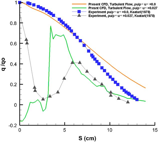
Figure 4 shows a comparison of the present results against the measurements from Kaattari⁽ Reference Kaatari ^{19 )}. As mentioned earlier, the computation was carried out for fully turbulent flows. No effects from transition mentioned in the experiment have been included. For the blowing simulation, no attempt has been made to simulate the ejection profile used in the experiment. It should also be noted that the increase in heating rate reduction in the experiment is consistent with the surface injectant flux profile that increases 50% from the stagnation point reaching a maximum near the heat flux minima. For the solid surface case, the computed heat transfer rates, while remaining fairly close to the experiment for the nose region tend to overpredict the heat flux towards the straight portion. The concentrated flow ejection in the close vicinity of the stagnation region leads to substantially lower values of heat transfer rates adjacent to the nose as opposed to the experimental results showing a maximum heat transfer rate at the apex followed by notable cooling, almost reaching the computed values at about 2.5 cm from the nose. The computed results show a maximum heat transfer at S≈3.5 cm, whereas the experiments show a second peak at S≈6.5 cm. Both computed and the experimental results for the flow ejection case remain very close beyond S≈6.0 cm, but always below heat transfer rate values for the solid surface case.

Figure 4 Heat transfer comparison with experiment, M=7.32, Re_D=1.1×10⁶.

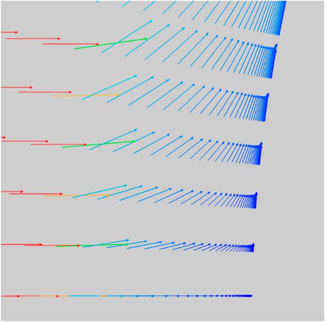
Figures 5 and 6 show the velocity vectors at the blunt surface near the stagnation region. Not only does the injectant flow cause a barrier between the surface and the free stream but also redirects the flow upstream of the body as the flow is decelerated. Note the change in the shape of the velocity profiles at the surface from blowing.

Figure 5 Velocity vectors (solid surface).

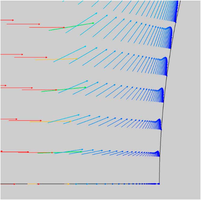
Figure 6 Velocity vectors flow ejection case ρu/ρ_∞ u _∞=0.027.

A round blunt-nosed cone ogive and a sharp blunt-nosed ogive cone were selected from the experiments carried out by Nowak⁽ Reference Nowak ^{20 )} as further two wind tunnel models to validate the present computational method. The computed Mach number flow field is shown in Fig. 7.

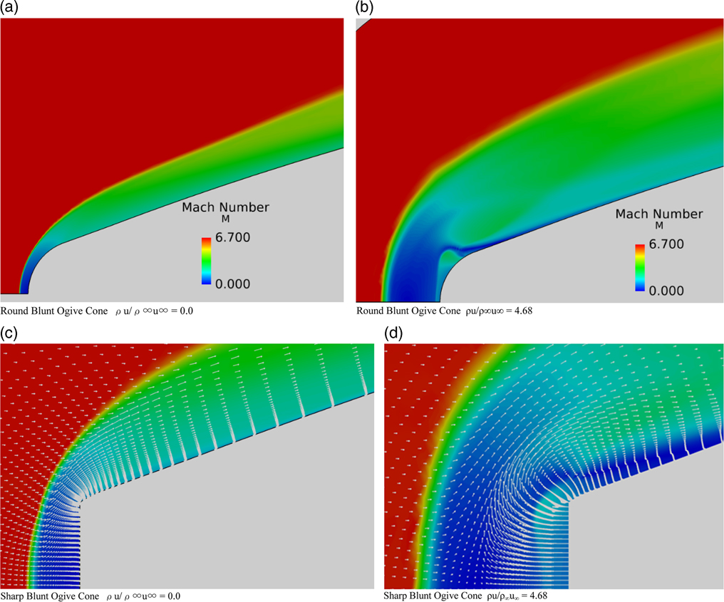
Figure 7 Mach number flow field, M=6.8, Re=1.3×10⁶, α=0.0°. (a) Round blunt ogive cone ρu/ρ∞u∞=0.0. (b) Round blunt ogive cone ρu/ρ∞u∞=4.68. (c) Sharp blunt ogive cone ρu/ρ_∞ u _∞=0.0. (d) Sharp blunt ogive cone ρu/ρ_∞ u _∞=4.68.

It is clear that the flow ejection has the effect of pushing the shock wave away from the nose. The flow field in the vicinity of the blunt nose is radically changed owing to blowing with large of areas of decelerated flow responsible for heat reduction. There is a larger region of decelerated flow between the shock and the blunt round nosed cone when ejection is applied. Note also the presence of the jet shock near the nose of the round nose airfoil. The momentum vectors superimposed upon the Mach number flow field for the sharp-nosed cone are shown in Fig. 7 (c) and (d) that there is the presence of strong recirculation and reversal of the flow near the sharp corner of the cone with a clear reattachment point downstream of the corner. The detailed flow field can also be compared with the shadowgraphs in Fig. 8, taken from Nowak⁽ Reference Nowak ^{20 )}. The solid nosed cone results match up closely with the experiment whereas the sharp-nosed results with blowing (ρu/ρ∞u∞=4.68) show a complex flow pattern in front of the nose. The distinct round contour next to the shock is the jet mainstream interface present in both computations and the shadowgraph. The jet normal shock too is visible in both pictures.

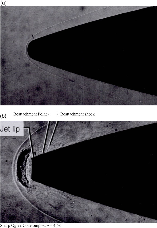
Figure 8 Shadowgraphs of round nosed and sharp nose ogive cones in hypersonic flow, Nowak (1988). (a) Round Blunt Ogive Cone ρu/ρ∞u∞ = 0.0. (b) Sharp Ogive Cone ρu/ρ∞u∞ = 4.68

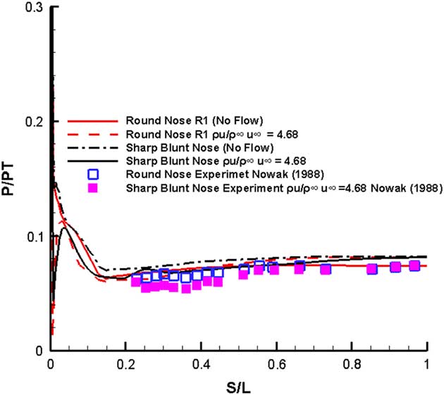
The pressure distribution comparison for the two models against the available experimental data is shown in Fig. 9

Figure 9 Normalized pressure distribution M=6.8, Re=1.3×10⁶, α=0.0°.

. For the round nosed ogive cone, only the solid surface results were available, whereas for the sharp nose, ogive cone only the flow applied data was available.

The round nosed computed results shown by the solid curve remain fairly close to the experimental data depicted by square symbols. The flow is understandably transformed near the nose by blowing but follows the solid body results away from the nose. The sharp-nosed solid surface results are somewhat higher than the corresponding round nosed cone results on most of the surface. The blowing on sharp-nosed results are different at the nose region, and are again a little higher than the corresponding experimental results represented by the filled squares.

The results from the heat transfer computations are shown in Fig. 10. The computed results on the solid body round nosed cone are represented by the solid line curve and they show an increasing heat transfer rate trend near the nose as indeed does the experimental data. The results on the surface away from the nose too are well matched. However, the computations do not resolve the notable depression in heat transfer rates just past the nose region. The flow ejection results indicated by the dashed curve show a notable decrease in heat transfer results near the nose before settling down to a value of q/q _o=0.05 away from the nose. The solid sharp-nosed cone consistently shows higher heat transfer rate than the solid round cone. The flow ejection results show lower values than the corresponding solid body results up to S/L=0.5 beyond which they show an increasing trend. The heat transfer experimental data for the flow ejection data for the sharp-nosed cone shows a decreasing trend near the nose which is the same as the computed results.

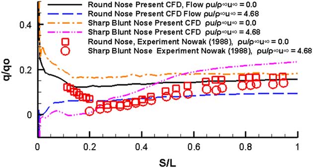
Figure 10 Heat transfer results M=6.8, Re=1.3×10⁶, α=0.0°.

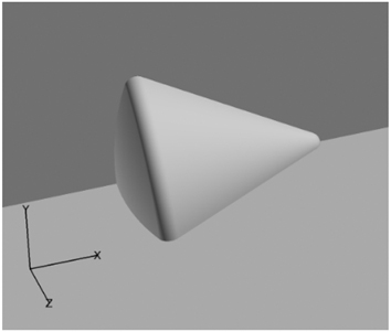
The next series of models examined the hypersonic flow past configurations which have been used in real-life projects. The first of these is the Venus–Galileo model shown in Fig. 11. It consisted of a blunt cone fore body of bluntness R _N/R _B=0.5 with a base diameter of 1 m and a conical surface of 45° half-angle which abuts smoothly on to a cylindrical shoulder which has a radius of 0.1 m. The dimensions of the forebody corresponded to the Pioneer–Venus–Galileo rocket as provided by Micheltree⁽ Reference Mitcheltree, Moss, Cheatwood, Greene and Braunq ^{11 )}. Figure 12 shows the single block of a mesh of dimensions 83×127×45 used for this simple forebody. The y+ value for the first grid line in the normal direction to the solid wall was kept in between 1 and 2 along the axial length of the model.

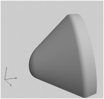
Figure 11 Pioneer–Venus–Galileo model.

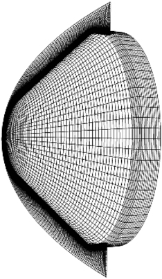
Figure 12 83×127×45 mesh.

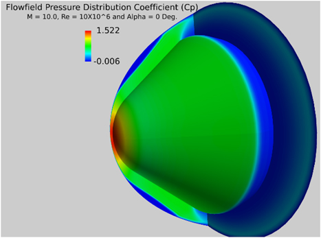
The pressure distribution at $M_{\infty} $ =10, α=0° and $R$ =10×10⁶ at the spherical blunt nose is shown in Fig. 13. In order to avoid sonic choking conditions at the outflow boundary, only a small mass flow ${{\rrho u} \over {\rrho _{\infty} u_{\infty} }}{\equals}0.01$ was tested for the blowing case in the nose region.

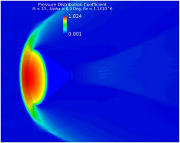
Figure 13 C _p distribution solid surface.

It can be seen that a very strong shock immediately upstream of the nose at a very small standoff distance which is very consistent with the flow at M=10. The blowing has a profound effect upon the pressure field in the vicinity of the nose and the introduction of the additional mass flow from the outflow boundary at a relatively higher static pressure dilutes the high stagnation region between the nose and the shock. A comparison of the computed pressure distribution against the experimental data extrapolated for a 45° blunt cone from Belotserkovskii and Chushkin⁽ Reference Belotserkovskii. and Chushkin ^{21 )} is given in Fig. 14.

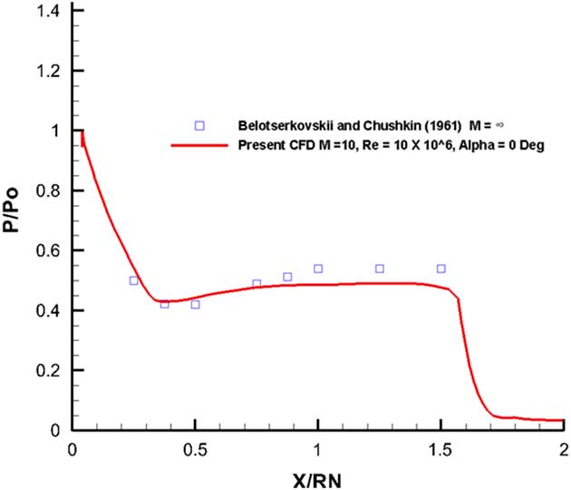
Figure 14 Pressure distribution on the blunt fore body, M=10, Re=10×10⁶, α=0°.

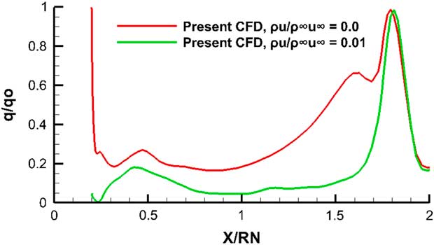
The agreement between the computed and the extrapolated data from Belotserkovskii and Chushkin⁽ Reference Belotserkovskii. and Chushkin ^{21 )} is quite satisfactory. The pressure distribution calculations for the leading edge blowing case follow the solid surface case quite closely and are not repeated here. The heat flux calculations were also carried out for this Galileo configuration. The heat flux values normalized with respect to the stagnation point using the Fay–Rayddell technique mentioned above are shown in Fig. 15.

Figure 15 Heat flux on the blunt fore body, M=10, Re=10×10⁶, α=0°.

Across the blunt nose region itself where the cooler air is just entering the flow field, the heat transfer rate as in the previous cylindrical nose model, is noticeably lower than the solid boundary case. The lower heat transfer rates established for the blowing case at the nose are carried through to the conical region until the shoulder location where the two results from the ejection case and solid boundary case equalize. The velocity contours near the blunt surface of the model for the solid surface and the blowing surface are shown in Figs 16 and 17. Note how the first contour for the blowing case indicates a reversed blowing flow at the blunt surface in place of the no-slip condition for the solid surface case.

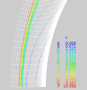
Figure 16 Velocity contours (solid surface).

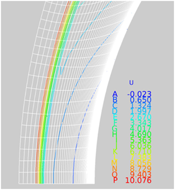
Figure 17 Velocity contours flow ejection case ρu/ρ_∞ u _∞=0.01.

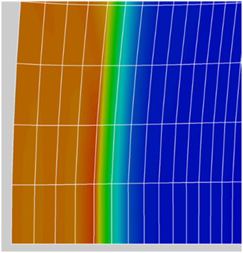
Figures 18 and 19 show the shock location in the Mach number flow field distribution near the blunt nose of the two cases under study. For the solid surface case in Fig. 14, the centre of the shock location identified as the red-yellow boundary is seen to be at grid point about 5.3 counting from the left. For the outflow case in Fig. 15, the red-yellow boundary appears to be relatively closer to grid point 5 from the left. The small outflow (ρu/ρ_∞ u _∞=0.01) has the effect of pushing the shock slightly away from the blunt nose.

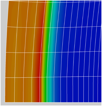
Figure 18 Shock location (solid surface).

Figure 19 Shock location, flow ejection case ρu/ρ_∞ u _∞=0.01.

The grid for the Apollo configuration (Fig. 20) as used in the present study is shown in Fig. 21. The 2D grid shown on the right-hand side was rotated through 90° to produce the 3D configuration. The basic dimensions for the grid were obtained from Moss et al.⁽ Reference Moss, Glass and Greene ^{12 )}. The y+ dimension on the surface remained less than 1 everywhere on the surface of the configuration.

Figure 20 Apollo configuration.

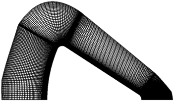
Figure 21 2D grid (100×121).

The CFD computation was carried out once again at M=10, Re=1.1×10⁶ and α=0 Deg. Figure 22 shows the pressure coefficient distribution on the model and the flow field.

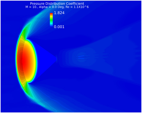
Figure 22 C _p distribution solid surface M=10, Re=1.1×10⁶, α=0°.

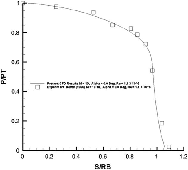
The pressure distribution obtained from the present solid surface case was compared against the measurement as reported by Bertin⁽ Reference Bertin ^{22 )} in Fig. 23.

Figure 23 Pressure distribution on the front spherical portion of the Apollo configuration.

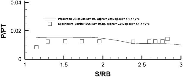
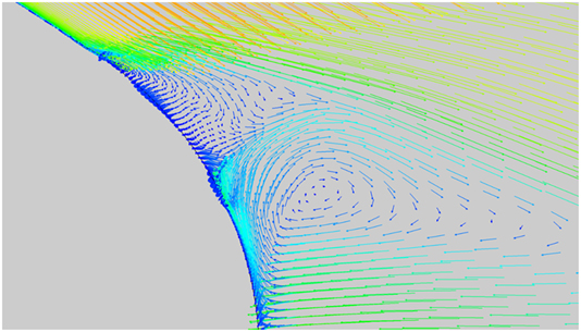
The agreement between the computed measured values and the experiment is very good for the front spherical surface. The back conical surface as shown in Fig. 24 suffers from large-scale flow separation at the trailing of the model which may not be well resolved by the current one-equation Spalart–Allmaras turbulence model. Even then the comparison of pressures as observed in Fig. 24 is quite good. The heat flux was also computed on the back surface of the configuration (Figs 25). A reversing separated flow would give rise to increasing heat transfer rates towards this region. A comparison of results for the front blunt surface against the experimental data is shown in Fig. 26. The flow ejection case shows heat transfer values lower than those for the solid surface. Within the error margin of the experiment, the computed results matched well with the measurements.

Figure 24 Pressure distribution on the back conical portion of the Apollo configuration.

Figure 25 Separated and reversing flow at the trailing end of the Apollo model.

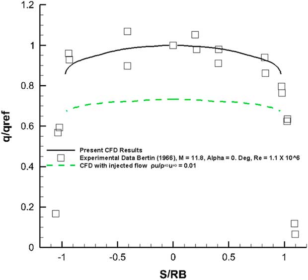
Figure 26 Heat flux on the blunt face, M=10, Re=1.1×10⁶, α=0°.

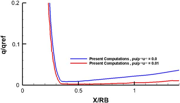
A comparison of the results between the flow injection case and the solid surface case for the back conical surface is shown in Fig. 27. It is clear that the heat transfer rate at the back conical portion is a small fraction of the heat transfer rate at the blunt region. The figure shows that the distances greater than 0.5 with injection reduces the heat transfer in the base of the body. This could possibly be due to the fact that the injectant defies the mixing imposed by the highly turbulent wake, or perhaps as indicated in Fig. 25, it acts as a barrier attached to the base.

Figure 27 Heat flux in the axial direction, M=10, Re=1.1×10⁶, α=0°.

Finally, CFD-based simulations were carried out to study the flow field past the X-38 Space Shuttle. The dimensions were taken directly from the published 3-view data (Fig. 28) from the literature^{( 23 )}. A cad model of the orbiter was produced from this figure. Since the details in the inner portions (especially the valleys in between the wing and the body) were only extrapolated from a blown up version of the simple drawing, it is difficult to say if the final model was as accurate. The various protuberance on the top surface were ignored to produce a simple model convenient for CFD simulations. The 3-view drawing used to reproduce the cad model is shown in Fig. 28 along with the 3D model displaying the surface grid which consisted of 12 blocks comprising some 175,000 grid points in Fig. 29.

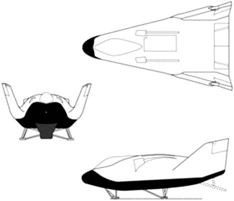
Figure 28 Length: 30 ft 0 in (36 ft including deorbit propulsion system rocket).

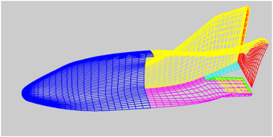
Figure 29 A simple X-38 CAD model showing the surface mesh.

The y+ values on the major blocks encapsulating the main geometry surfaces are shown in Fig. 30. Every effort was made to keep on y+ value close to below 1 for the bottom surface where most of the heat transfer occurs.

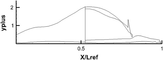
Figure 30 y+ distribution across the surface of the X-3D Space Shuttle Orbiter.

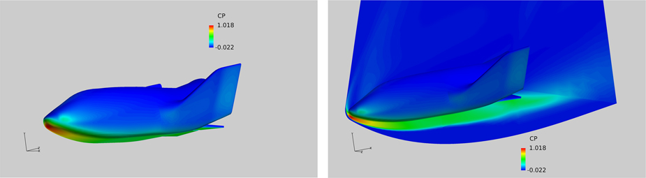
The flow field pressure distribution obtained on the X-38 surface is shown in Fig. 31. Figure on the left-hand side shows the pressure distribution on the complete model. The figure on the right includes the pressure field on a reflection plane running through the centre of the model.

Figure 31 C _p distribution solid surface, M=8, Re=8.1×10⁶, α=40°.

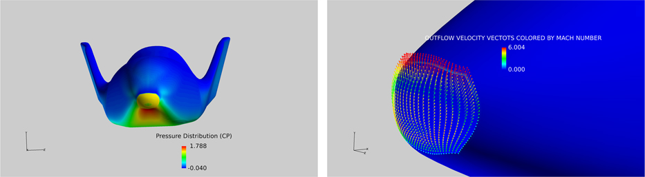
It is noted that region of high pressure exists near the nose of the model with the stagnation point well below the nose. The flow field across the reflection plane confirms that most of the flow activity is concentrated on the lower pressure side with the pressures on the leeward side drop to low values immediately past the nose region. Figure 32 shows the pressure field where the exit pressure at the nose boundary was fixed to give an outflow M_out=0.3. The exit pressure was calculated by considering the flow Mach number and pressure at the edge of the boundary layer. The static pressure was then calculated to give a M_out=0.3 at the surface. The outflow from the solid boundary is immediately affected by the flow accelerating round the blunt nose and the resulting velocity field at the solid surface is shown on the right-hand side of Fig. 32. It is, of course, obvious that no such velocity vector field is available for the solid boundary case.

Figure 32 C _p distribution (left) and the velocity vectors (right) with flow injection at the leading edge, M=8, Re=8.1×10⁶, α=40°, M_out=0.3.

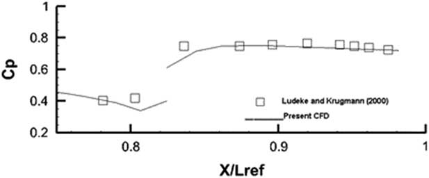
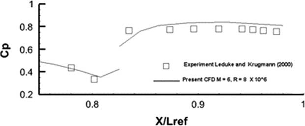
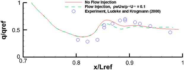
The computed pressure distribution at M=6 and Reynolds numbers Re=3.1×10⁶ and 8.1×10⁶ were compared against measurements taken from Leduke and Krogmann⁽ Reference Ludeke and Krogmann ^{24 )}. For the lower Reynolds number Re=3.1×10⁶, the computations were conducted for a laminar flow as indeed was done in Ref. Reference Ludeke and Krogmann24. For the higher Reynolds number Re=8.1×10⁶, Spalart–Allmaras one equation was used for the complete model. Transition fixing was not attempted as the present solver as yet is not equipped with the capability. The comparison for both flows is shown in Figs 33 and 34.

Figure 33 C _p distribution M=6, Re=3.1×10⁶, α=40°, laminar flow.

Figure 34 C_p distribution M=6, Re=8.1×10⁶, α=40°, turbulent flow.

It appears that for this laminar flow case in Fig. 35, for the outboard station cut, the comparison with experiment is quite good. In the region between 0.8<X/L _ref<0.84, the flow is separated and reversing. Still, the agreement between computed results and measurements is good. The disconnect in the pressure curve at X/L _ref~0.815 is due to the fact that almost two coincident points lie on two adjacent blocks where the first point is on the main body and the second point is on the flaps defected at 20^○. Figure 34 shows the same comparison case for a turbulent flow at Re=8.1×10⁶. Once again the one equation Spalart–Allmaras turbulence model has done reasonably well in being able to resolve this turbulent flow. Since the cad model was produced from dimensions extrapolated from a 3-view technical it is quite possible that there were some small differences between the current model and the exact geometry used in the experiment. The comparisons, however, are very encouraging. The heat flux results with and without the boundary outflow are shown in Figs 35 and 36. The stagnation point value of the heat flux (q _ref) was used to normalize the results. It must, of course, be mentioned that the present method does not account for any diffusion, flow dissociation or other radiative effects.

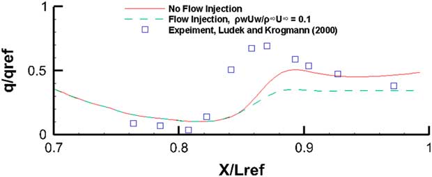
Figure 35 Heat flux, M=6, Re=3.1×10⁶, α=40°, laminar flow.

Figure 36 Heat flux, M=6, Re=8.1×10⁶, α=40°, turbulent flow.

For the laminar flow case in Fig. 35, the computations follow the general experimental trends quite faithfully. Only in the flow separation region just before the flaps, it is unable to resolve the higher level of heat activity. The outflow case depicted by the dashed lines indicate that even with this high angle-of-attack (α=40°), where the tendency for the injected out flow is to move towards the leeward side, the blowing does appears to alleviate the heat flux. For the turbulent case in Fig. 36, there is an encouraging attempt by this one-equation model to come fairly close to the experimental values. The blowing off course has not performed as well as the earlier laminar case.