

Introduction
The 1996 Personal Responsibility and Work Opportunity Reconciliation Act (PRWORA) replaced Aid to Families with Dependent Children (AFDC), an entitlement program that provided cash assistance to very poor families, with the Temporary Assistance to Needy Families (TANF) block grant program. The primary goal of the reformed program was to end the dependence of needy families with children on government benefits by promoting and supporting employment. Under TANF, most able-bodied recipients are required to participate in work or work-related activities for a minimum number of hours per week. In addition, for most families, benefit receipt is limited to five years in a lifetime. South Carolina implemented its own TANF-funded program, Family Independence (FI), in October 1996. Similar to the TANF programs in many states, FI embraces a ‘work first’ approach, which prioritizes moving recipients into employment as quickly as possible. Important FI program components include both incentives (e.g. work support and earning disregards) and penalties (e.g. sanctions for failure to comply with work requirements and shorter time limits for benefit receipt than those required under federal law).
Between 1996 and 2000, the number of TANF families in the United States, mostly headed by single mothers, declined from 4.5 million to 2.2 million. While caseloads plummeted, the employment rate among women most affected by PRWORA increased markedly. Among the first evaluative studies of the welfare reform era were ‘leaver surveys’ initiated by the South Carolina Department of Social Services (SC DSS) in 1996. Based on eight quarters of surveys, agency researchers reported that approximately 70% of former recipients were working after exiting FI, and most did not report suffering deprivations (Edelhoch, Reference Edelhoch1999). In 1998, the US Department of Health and Human Services (DHHS) Office of the Assistant Secretary for Planning and Evaluation (ASPE) funded leaver surveys in 13 states, including in South Carolina, using standardized research instruments. These studies showed that the majority of clients who left cash assistance since the enactment of TANF were working, and most were working at least 30 hours per week (Acs et al., Reference Acs, Loprest and Roberts2001).
Welfare reform evaluations conducted during the early years of TANF have been reviewed by Blank (Reference Blank2002, Reference Blank, Card and Quigley2006), Moffitt (Reference Moffitt2008), and Gueron and Rolston (Reference Gueron and Rolston2013), among others. Moffitt (Reference Moffitt2008) concluded that the reform had generally positive average effects on employment, earnings, and income, and generally negative effects on poverty rates. However, the economic gains were not evenly distributed across groups (Moffitt, Reference Moffitt2008; Wood et al., Reference Wood, Moore and Rangarajan2008; Pavetti and Schott, Reference Pavetti and Schott2011). For example, sanctioned clients were significantly less likely to be employed and, even when employed, earned significantly less than other clients did (Edelhoch et al., Reference Edelhoch, Martin and Liu2000).
Some researchers and policy analysts have argued that strong economic growth played a significant role in the increased labor market participation during the early years of TANF. Determining the success of welfare reform, according to Blank (Reference Blank2002, Reference Blank and Zilliak2009), depends on gauging the program’s performance during a significant economic downturn. Surprisingly, the recession that began in 2001 did not lead to either much larger increases in the unemployment rate or to much higher TANF participation among lower-skilled single mothers. It could have been that TANF recipients had better access to job search assistance and work support programs than other unemployed persons had. In addition, the recession was relatively mild and short and had only a limited impact on job sectors where low-skilled women were most likely to be employed (Blank, Reference Blank, Card and Quigley2006).
During the 2007-2009 recession, however, unemployment rates in South Carolina increased from less than 6% to over 12%. This recession has provided South Carolina researchers an opportunity to evaluate the state’s FI program during a serious and widespread recession. The purpose of this study is to address two research questions. First, what was the impact of participation in the FI program on participants’ earnings? Second, if FI intervention resulted in higher earnings for participants, how did the impact vary as the economy moved from relative health and stability to a deep recession? We hypothesized that participation in FI accelerated earnings growth for program participants, but that the program impact weakened during periods of economic downturn.
We compared the earnings trajectories of three cohorts of matched treatment and comparison groups who applied for FI before, at the beginning of, and at the height of the recession. Our original treatment group consisted of applicants approved to participate in FI. Our original comparison group came from applicants who did not complete the application (41%), who voluntarily withdrew their application (33%), whose resources or income exceeded the limit (17%), or who were deemed ineligible (10%).Footnote 1 The matching was conducted by modeling the likelihood of FI entry based on preintervention earnings history, county unemployment rate, and family and individual demographic characteristics.
We used a latent growth curve model (LGCM) to test our hypotheses. Our major finding is that while the FI program increased the earnings of participants before the recession, similar effects were not observed for cohorts that entered FI during the recession. We conclude with a discussion of changes that could make the program more responsive to cyclical changes in the economy and of the importance of strengthening FI both as an employment program and a safety net.
South Carolina’s Family Independence Program
Similar to most other states, South Carolina employed a work-first approach that emphasized placing participants into jobs as quickly as possible. For initial eligibility, FI required applicants to make five job contacts in two weeks while applications were processed. Once the application was approved, those deemed employable were required to participate in structured classroom activities for two weeks during which FI staff assessed participants’ job skills; informed them of the program policies, work requirements, work-support services and transitional benefits; and provided training in job search techniques, resume development, and interview skills. After training, FI participants engaged in self-directed job searches with the assistance of case managers for up to eight weeks.
The array of activities available to participants who were unsuccessful in finding employment after eight weeks of job search varied by county and job market. The most common options included short-term job-skills training, on-the-job training, family life-skills training, community service, volunteer work, and the Work Experience program, in combination with job search. A small number of individuals with complex barriers to employment were referred to outside agencies for vocational rehabilitative services, substance abuse treatment, mental and physical health services, and housing assistance.
In general, South Carolina’s FI program was designed with some of the strictest work requirements and least generous cash benefits of the state and local TANF programs in the country.Footnote 2 South Carolina implemented a 24-month time limit in ten years, which was stricter than the federal limit of 60 months, and instituted ‘full family sanctions’ in cases where the client did not follow program rules, which suspended the entire benefit until the sanction was lifted. In 2007, FI benefits for a family of three with no income in South Carolina were still only $205 per month (as they had been since the start of FI), compared with the median amount of $389 for all states. The low cash benefits meant FI recipients were on average relatively disadvantaged, with perhaps greater incentives to seek entry-level employment than to rely on assistance (Acs et al., Reference Acs, Coe, Watson and Lerman1998).
In June 2006, in accordance with the 2005 Deficit Reduction Act (DRA), the US DHHS issued new regulations requiring more stringent application of the TANF work requirements. As a result, South Carolina narrowed the definition of FI work activities, restricted exemptions from work participation to a limited number of families in a state-funded program, and trained staff about changes under the new legislation. Toward the end of 2006, compared with earlier years, FI administrators and staff were more experienced, and percentage of the caseload participating in work and work-related activities remained satisfactory and steady.
In summary, states took advantage of the flexibility offered by the federal block grants in structuring their own cash public assistance programs, but shared the basic features of work support programs – assistance with job readiness and job search, subsidies for transportation and childcare expenses, and case management. In addition, South Carolina’s FI program shared a fundamental similarity – a work first approach – to most other TANF programs, focusing on clients getting a job, rather than providing job-related education and/or training.
Literature Review
Effect of Reform
As the primary goal of the 1996 reform was to end dependence on cash assistance by promoting job preparation and work, much of the early research focused on the effects of TANF on caseloads and employment. As noted earlier, the weight of the research has indicated that the reform led to significant declines in welfare participation and increases in single-mother employment and earnings (Blank, Reference Blank2002, Reference Blank, Card and Quigley2006; Moffitt, Reference Moffitt2008; Gueron and Rolston, Reference Gueron and Rolston2013).
In the United States, the most influential evidence for the effect of welfare reform on employment outcomes came from the pre-TANF welfare-to-work experiments, known as the National Evaluation of Welfare-to-Work Strategies (NEWWS). NEWWS used a rigorous experimental design to study the effects of eleven welfare-to-work programs in seven states. A synthesis of the reported effectiveness of three major intervention approaches (work-first, education-first, and mixed) provided strong evidence that all three approaches increased employment and earnings compared with no program (Hamilton and Scrivener, Reference Hamilton and Scrivener2012). Over five years, the average earnings of the work-first groups were $1,500 to $2,500 greater than those of the control groups (US DHHS and US DOE, 2001). These positive findings and the rigor with which the evaluations were conducted were a major reason PRWORA became law in 1996.
Prior to US TANF reform, Canada shifted from a single centralized social assistance (SA) system to multiple decentralized SA programs. Unlike in the US, where most states implemented TANF within a few months of each other and employed a work-first approach, Canada’s new reform strategies were administered very differently across provinces and over time. The differential timing and types of reform enabled Canadian researchers (Berg and Gabel, Reference Berg and Gabel2015, Reference Berg and Gabel2017) to test the effects these policy changes had on the nation’s social assistance rates and on an array of other reform outcomes. A mixture of aggregated province-level data and individual-level data allowed for a decomposition of changes in SA participation into portions attributable to macroeconomic variables, to individual idiosyncratic factors, and to welfare reform policy. The results of the analyses showed that the aggregate effect of the reform’s four major strategies (work requirements, diversion, earnings exemptions and time limits), more than the macroeconomic and individual factors, was responsible for the significant reductions in Canada’s SA participation. Within the new reform strategies, work requirements with strong sanctions had the largest effect on the reduction of the SA caseload.
In the spirit of the Europe 2020 Strategy, improving the quality of work and employment has been part of the agenda of European-style labor market reforms. To determine whether Germany’s ‘new welfare’ that put stronger emphasis on labor market participation created ‘more and better jobs’, Dengler (Reference Dengler2019) evaluated the effects of the country’s four major active labor-market programs (One-Euro-Jobs, short-term classroom training, short-term in-firm training, and further vocational training) on participants’ job quality. Job quality was defined and measured by job type, job stability, integration into regular jobs, income, self-sufficiency, and working conditions. The results showed that all four programs (even ‘One-Euro-Jobs’, provided as a last resort to the hard-to-place welfare recipients) increased participants’ probability of holding a high-quality job relative to the matched controls. Further vocational training – a long-term qualification program that provides professional and practical job-skills training – is remarkably effective at increasing participants’ likelihood of obtaining regular jobs, remaining in the job market, and staying off public assistance.
The Policy versus Economy Debate
In the US, evaluations sponsored primarily by the federal government and conducted at research institutes, policy centers, universities, and state government agencies have contributed greatly to understanding the effects of TANF policies. However, some important questions about the extent to which the strong US economy in the late 1990s contributed to the TANF caseload decline and to the increase in employment remain unanswered. Most studies that have attempted to assess the relative importance of the policy vs. the economy have suggested that both the policy changes and the economy had an impact, but the magnitude of the estimated impact has varied considerably (Blank, Reference Blank2002, Reference Blank, Card and Quigley2006; Ziliak, Reference Ziliak and Moffitt2016). One reason these studies have provided inconsistent results is because, with very few exceptions, they relied heavily on national survey or state panel data from the years around the implementation of state TANF programs when levels of unemployment were relatively low and stable.
In a 2007 discussion of future research needs, Blank (Reference Blank and Zilliak2009) noted: ‘the most obvious way’ to study the differential effects of the policy and the economy would be ‘to wait for the next economic slowdown and see what changes’. That unfortunate opportunity materialized during the 2007-2009 ‘Great Recession’. The recession led to renewed calls to evaluate the effects of TANF throughout its history, especially during the recession (Pavetti and Schott, Reference Pavetti and Schott2011). However, thus far, there has not been much research effort along these lines. Given the availability of high-quality administrative data and recent advancements in longitudinal modeling methods, researchers are now in a much better position to elucidate the relationship between the economy and the program.
Strategies to Increase the Rigor of Non-Experimental Studies
Evaluation methodologists and researchers have been exploring methods to strengthen nonexperimental approaches to assessing the effectiveness of program interventions. The key challenge is to find the method that best estimates the counterfactual. A widely used method is to compare the outcomes for a sample of the program participants with a sample of nonparticipants whose observed characteristics are closely matched.
Researchers who compare impact estimates of programs with both an experimental and a nonexperimental component have typically found that estimates based on matched samples are closer to experimental benchmarks than estimates based on unmatched samples (Dehejia and Wahba, Reference Dehejia and Wahba1999). Among the various methods, propensity-score matching (PSM) has been widely used by researchers from a variety of disciplines. PSM works significantly better when important covariates, such as pretests or preintervention labor market histories, are used than when only generic predictors such as sex, age, marital status, and ethnicity are used (Shadish et al., Reference Shadish, Clark and Steiner2008). It is important to note that although matching can significantly increase the internal validity of a study, matching cannot eliminate selection bias completely due to unmeasured factors that differ between the groups related to the reasons that they are exposed or unexposed to the intervention.
Another way to reduce selection bias is to draw treatment and control samples from either the same, or a very similar, population (Shadish et al., Reference Shadish, Cook and Campbell2002). The usefulness of this approach was demonstrated in the evaluation of an applicant-based training and work program executed both as a randomized controlled trial (RCT) and as a non-RCT (Bell et al., Reference Bell, Orr, Blomquist and Cain1995). The RCT control group consisted of eligible applicants who were initially approved to receive services before being randomly assigned to the control group, which would receive no services. The non-RCT control group consisted of eligible nonparticipants – applicants who withdrew their applications, or who were screened out. Analyses comparing the treatment group with the RCT and non-RCT controls reached the same conclusion: compared with both the RCT and non-RCT control groups, the treatment group made faster gains in earnings during the follow-up period. The study’s conclusion is convincing because, by selecting the treatment and non-RCT control groups from individuals who sought to participate in the training program, the group members were very similar in terms of labor market experiences and other demographic characteristics known to influence employment outcomes.
Designs that use longitudinal data ‘often represent our best approaches to evaluating causal relations’ in situations where it is not possible or ethical to manipulate the presumed cause (Card and Little, Reference Card and Little2007). The richer information drawn from multiple-waves of data, as opposed to data drawn from a specific time, allows for estimation of changes with more precision and reliability (Willett, Reference Willett1989). Furthermore, multiple-waves of data collected on the outcome measures before intervention can be used to effectively establish baseline equivalency. For example, Dehejia and Wahba (Reference Dehejia and Wahba1999) demonstrated that when preintervention earnings over two years – rather than one year – were included in the matching protocol for generating treatment and comparison groups, the impact estimates were more reliable. This finding led the authors to recommend using lengthy baseline earnings in evaluating employment and training programs. Longitudinal data also offer the possibility of studying cohorts of individuals before and after major historical events, such as a recession (Connelly et al., Reference Connelly, Playford, Gayle and Dibben2016). Provided the population of interest does not change dramatically, researchers can use the earlier (or later) cohort as a comparison group to examine changes attributable to the event.
Impact studies without randomization are not equivalent in their ability to estimate an intervention’s causal effect. Based on a systematic review of the published literature in various disciplines such as education and anthropology, Shadish et al. (Reference Shadish, Cook and Campbell2002) ranked major study designs to reflect increases in inferential power. They situated studies without a comparison group or a pretest on the low end, those with both in the middle, and the interrupted time series design on the high end. One of the advantages of employing an ‘interrupted time series design’ is that, with multiple measurements before and after an intervention, it is easier for researchers to address selection bias and regression to the mean (Harris et al., Reference Harris, McGregor, Perencevich, Furuno, Zhu, Peterson and Finkelstein2006). Most of the designs can be strengthened by incorporating other features, such as adding untreated matched controls to the basic interrupted time series designs (Shadish et al., Reference Shadish, Cook and Campbell2002).
Methodology
Data Sources
Our study employed program and earning records from two sources. The first was the SC DSS administrative database from which we obtained the dates of FI applications, the beginning and ending dates of each FI spell, the beginning and ending dates of each Food Stamps spell, residential county and other demographic characteristics. The second data source was quarterly unemployment insurance (UI) wage data for most South Carolina employees.Footnote 3 We constructed a data file from these two sources that contained UI information over seven quarters for each single mother in the sample, thereby tracking her earnings before and after possible entry into FI. We used each household’s county of residence to obtain the county unemployment rate over the same seven quarters as an indicator for economic conditions.
Sample
Samples for this study were selected from three cohorts of single parents between the ages of 19 and 55 who applied for FI during February and MarchFootnote 4 of 2007 (pre-recession), 2008 (early recession), and 2009 (height of the recession) and who received food stampsFootnote 5 in the month of FI application or the month prior to FI application. Because the number of new entrants and labor market opportunities tended to fluctuate seasonally, we sampled families that applied for FI during the same quarter in each of the three years. We selected cohorts from the years after FI implemented the changes required by the 2005 DRA and before operational practices in the agency were changed significantly in 2010 to ensure these changes either affected all or none of the cohorts. Importantly, the spacing of the three cohorts allowed us to study them when local unemployment rates were, respectively, low and stable, rapidly rising, and historically high.
After intake workers compared applicant needs to agency intake standards, fewer than half were approved for the FI program. We drew our initial treatment group from applicants approved to participate in FI who stayed on FI for at least three months after the intake decision was made (largely to exclude cases that were opened in error). We drew our initial comparison group from applicants who did not complete the application, whose resources or income exceeded the limit, or who were deemed ineligible. Similarly, members of the initial comparison group must not have accessed FI for at least three months after the decision (largely to exclude cases that were closed in error and reopened).
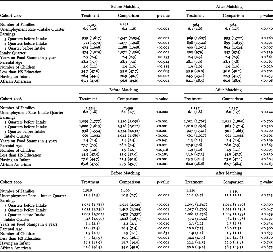
To construct the matched treatment and comparison groups, we first used a logistic regression model to predict each applicant’s probability (i.e. propensity score) of approval (yes = 1). We then selected treatment and comparison samples by matching two applicants without replacement, one from the original treatment group and one from the original comparison group, if their predicted approval probabilities (between 0 and 1) were closest and agreed up to three digits.Footnote 6 Table 1 provides descriptive statistics of the baseline covariates that were used to predict the probability: county unemployment rate, four quarters of UI earnings, years on food stamps in the past five years, parental age, number of children, and indicators (yes = 1) for whether the applicant had less than high-school education, had responsibility for an infant and was African American. As seen in Table 1, before matching, the treatment groups were more economically disadvantaged than the control groups. They were more likely to reside in counties with higher unemployment rates, to have lower earnings, and to have relied on food stamps longer. In addition, the treatment groups were more likely to have less than a high-school education, to have an infant, and to be African American.
Table 1. Means and Standard Deviations (in Parentheses) of Baseline Covariates

Note: UI Earnings includes $0 values for those with no UI Earnings.
The propensity-score model, run separately for each application cohort, yielded three sets of matched samples: 964 pairs for Cohort 2007, 1,137 pairs for Cohort 2008, and 1,336 pairs for Cohort 2009. After matching, the initial differences between the treatment and comparison groups either became statistically insignificant or were narrowed. The most important reduction was in preintervention earnings, where the clear advantage seen in the comparison group was almost completely eliminated. Earnings of within-cohort treatment and comparison groups also declined at a similar rate. The decline reflected the rate at which sample members became unemployed.Footnote 7 Statistically, the matched treatment and comparison groups were equivalent with respect to all the variables used for matching. Across the cohorts, the samples were comparable in earnings at intake, parental age, number of children, years on food stamps, percentage with less than high school education, percentage with an infant, and percentage African American. The only exception to this across-cohort similarity was in the baseline unemployment rate (6.3% for Cohort 2007, 6.1% for Cohort 2008, and 11.1% for Cohort 2009) and, not surprisingly, in the number of families needing government assistance.
The tradeoff for having created matched treatment and comparison groups is that they no longer mirror the original treatment and comparison groups. Of the single mothers in the initial 2007-2009 treatment groups, 964 (74 %), 1,137 (73%) and 1,336 (75%) were selected for subsequent analysis. As a result, and strictly speaking, estimates of the program impact are only meaningful for those in the matched samples.
Exploratory Data Analyses
Table 2 provides the unemployment rates and earnings for the matched treatment and control groups for the follow-up period (the three quarters following intake) by cohort. The top panel shows that the two matched groups were well balanced on unemployment rates for the quarter of intake (which was used as a predictor in calculating the propensity score) and the three subsequent quarters. The bottom panel shows that the earnings of all groups increased in a linear manner during the follow-up period, although rates of increase varied.
Table 2. Post-Intake Earnings and Unemployment Rates: Comparison of Matched Samples

Figure 1A-C shows earnings trajectories over the seven-quarter span for FI entrants (matched treatment group) and non-entrants (matched comparison group)Footnote 8 against state unemployment rates (bars) by cohort. For both the entrants and non-entrants, the earnings trajectories display a decreasing pre-intake trend, a turning point, and an increasing post-intake trend. The decreases in earnings before intake are remarkably similar between the entrants and non-entrants. After intake, the increase in earnings of the non-entrants represents a ‘normal recovery’ that would have occurred for the entrants had they not joined FI. If the FI program indeed made a positive impact, we should see UI earnings increase more rapidly for the entrants relative to the non-entrants. As expected, this is the case for Cohort 2007. Although the average earnings of entrants were initially at the same level as those of the non-entrants, their quarterly earnings were $305 more than the non-entrants by the end of the follow-up period (Figure 1A).
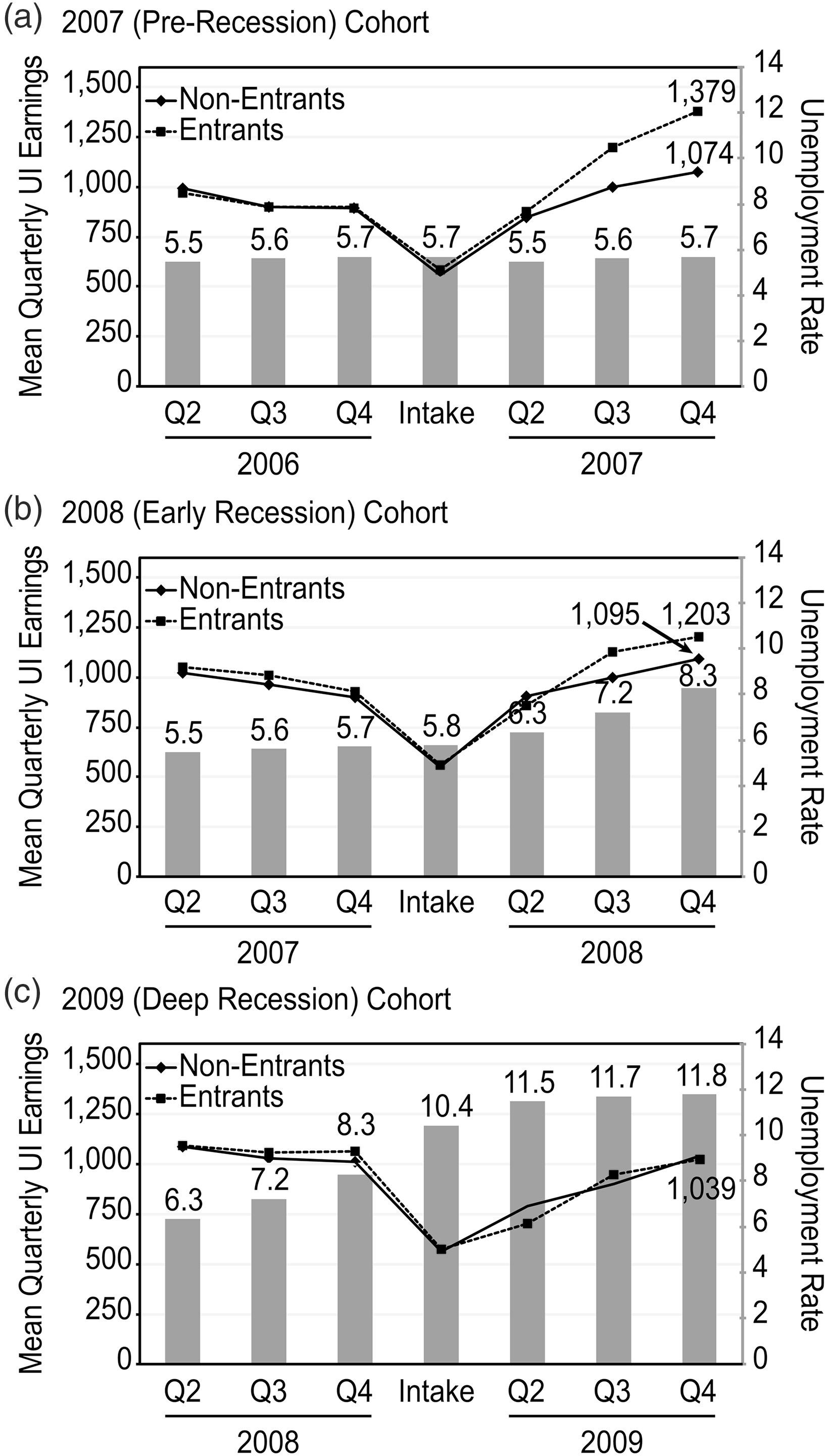
FIGURE 1A–C. Earnings of entrants and non-entrants before and after intake, by cohort.
Figure 1B and C illustrates the effect of the deterioration of the economy on the earnings of Cohort 2008 and Cohort 2009, as well as either little or no difference between the entrants and non-entrants in post-intake earning trajectories. By the end of the follow-up period, the advantage of the entrants over the non-entrants was only $108 for Cohort 2008 and was literally zero for Cohort 2009.
Latent Growth Curve Modeling
Figure 1A-C shows that the ‘preprogram dip’ and baseline earnings were markedly similar for the entrants and non-entrants and that the earnings gains after intake were different for Cohort 2007. To formally test whether what we see in Figure 1A-C arose by chance, we needed a statistical model that allows for (1) the earning trajectories to be different before and after intake, (2) the estimation of FI impact (the difference between the entrants and non-entrants in post-intake earnings trajectories), and (3) the estimation of the differences in FI impact across the three cohort groups.
We employed a multiple-group, two-piece latent growth curve model within the framework of structural equation modeling to fit our data. In our LGCM, the earnings of sample members were hypothesized to vary in terms of intercepts (representing initial status) and slopes (representing change), with the shape of slope reflected in the pattern of loadings. The model defines the intercept as the point joining the pre-intake and post-intake sections of the earnings trajectory; defines the shape of the first slope with factor loadings −1, −0.9, −0.8, and 0;Footnote 9 and defines the shape of the second slope with factor loadings 0, 1, 2 and 3.
We began by entering the county unemployment rate into the model as a predictor of earnings at each point in the seven-quarter span to control for the influence of the local economy in the estimation of the intercepts and slopes. In the next step, an indicator variable where 1/0 stands for participating/not participating in FI was included as a predictor of the intercepts and slopes. In addition, the model includes the following variables as predictors of the intercepts: indicators for having less than a high-school education, having an infant, and being an African American, and measurements of participants’ number of children and number of years on food stamps in the past five years.
Among all the parameters of this model, of primary interest is the differential effect of participating in FI on the post-intake slopes, i.e. the impact of FI. First, a positive and statistically significant difference would provide evidence that FI elevated earnings among the entrants above and beyond the normal recovery common to the entrants and non-entrants. Second, the presence of cohort differences in effect size would support our hypothesis that the impact of FI depends on the economic environment.
To test for differences in the impact of FI across cohorts, we began with separate-group analyses to assess how well our proposed latent growth model, described above, fit the data for each cohort. We used two fit indices – standardized root mean square residual (SRMR) and root mean square error of approximation (RMSEA) – to determine model fit. If the values of SRMR and RMSEA were under 0.08, we judged the model acceptable and used it as our base model to test whether the multiple-group model that restricted the parameter for FI impact to be the same across cohorts had the same fit as the model that allowed the parameter to be estimated freely. We used a chi-square difference test to compare the two multiple-group models. Additional chi-square tests were used to determine whether cohorts were similar in their mean intercepts, in their mean slopes, in the association between FI participation and the intercepts, and in the association between FI participation and the pre-intake slopes.
Results
Separate-Group Analysis
The model fit statistics indicated an excellent fit for the base model for each of the three cohorts according to SRMR (0.027, 0.024, and 0.025) and RMSEA (0.043, 0.036, and 0.038). For the three cohorts, the model-estimated parameters showed that the average earning trajectories (1) declined nonlinearly before intake, (2) increased linearly after intake, and (3) did not differ between the entrants and non-entrants before intake. For the 2007 non-entrants, earnings decreased to a total of $621 over the pre-intake period (t = 5.37, p < 0.01). Of the total decrease, approximately 10% occurred in each of the first two quarters, and approximately 80% occurred in the quarter immediately before intake. From intake to the end of the follow-up period, earnings increased to a total of $876, at a rate of $292 per quarter (t = 5.78, p < 0.01). The earnings of the 2007 entrants before intake followed essentially the same nonlinear trend as the non-entrants (t = 0.57). After program entry, the entrants earned an additional $94 each additional quarter (t = 3.50, p < 0.01). This increase, as a measure of FI impact, was only $36 (t = 1.46) for the 2008 entrants and $0.20 (t = 0.01) for the 2009 entrants.
Not surprisingly, the data clearly show a largely negative association between unemployment rates and earnings. In general, members of the three cohorts looking for jobs in high unemployment areas and/or during a recession were at a serious disadvantage. Even during better times such as those experienced by the 2007 entrants, an increase in the unemployment rate by two percentage points toward the end of the follow-up period reduced average quarterly earnings by $100.
Three demographic indicators – having a secondary or post-secondary education, having longer food stamps spells, and being African American – were associated with higher intercepts. Having more children and having an infant did not appreciably influence the intercepts. The reason that length of food stamp receipt was positively associated with initial earnings could be that families with shorter periods of food stamp participation might have been younger and hence had relatively shorter employment histories and lower earnings. It is not clear why African American applicants initially had higher earnings than applicants who were white and/or of other ethnicities. It is possible that a higher proportion of African Americans worked in the quarter of intake than individuals of other ethnicities, but their income did not exceed the eligibility limit.
Multiple-Group Analysis
The results from the multiple-group analysis confirm the existence of an interaction effect between FI intervention and the economy, as suggested by the separate-group analysis. The model that restricts the effect of FI participation on earnings progress to be the same across cohorts fit the data worse than the model that allowed the effect to take on different values (χ2 = 7.45, df = 2, p < 0.023). The difference in the effect of FI was significant between Cohort 2007 and Cohort 2009 (χ2 = 7.59, df = 1, p = 0.006), but was not significant between Cohort 2007 and Cohort 2008 (χ2 = 2.49, df = 1, p = 0.15). The experiences of the three cohorts were otherwise very similar. Statistically, they share the same intercept (χ2 = 5.64, df = 2, p = 0.06), the same pre-intake slope (χ2 = 2.34, df = 2, p = 0.30), the same post-intake slope (χ2 = 0.26, df = 2, p = 0.88), the same association between FI participation and the intercept (χ2 = 0.13, df = 2, p = 0.93), and the same association between FI participation and the pre-intake slope (χ2 = 0.26, df = 2, p < 0.88).
In summary, the LGC modeling analysis showed that South Carolina’s FI program successfully increased earnings among participants before the recession. Program impact lessened as the economy weakened. During periods of high unemployment, the FI program did not result in higher earnings for the participants relative to those of the comparison group who were without FI assistance.
Discussion
Several design features and the use of more recent data allowed this study to reach more definitive conclusions than some previous studies that have focused on employment outcomes post welfare reform. Longitudinal data from the SC Data Warehouse allowed us to follow three cohorts of FI program participants and nonparticipants, one before and two during the 2007-2009 recession, thereby distinguishing between changes due to labor market fluctuations and changes due to FI. We drew our treatment and comparison samples from cohorts of applicants and employed an interrupted time-series design with matched comparison groups to address selection bias and regression toward the mean. In addition, the longitudinal nature of the data allowed us to employ LGCM to explore the relatively complex relationships among variables. Compared with traditional analytical approaches for longitudinal data, LGCM techniques do not make some of the unrealistic technical assumptions, use more of the information available from the measured variables, and allow for more flexibility for examining research questions (Hancock et al., Reference Hancock, Harring, Lawrence, Hancock and Mueller2013). Increasingly, LGCM is recognized as one of the most powerful and informative approaches available for analyzing longitudinal data.
As is the case with evaluations that focus on one state and/or a specific time period, the findings of this study may be limited in their representativeness and may not generalize to other state programs, to other phases in TANF history, or to other economic cycles. Despite the measures we have taken to strengthen the design, we may not have sufficiently controlled for the influences of confounding factors. Nevertheless, the findings of this study do demonstrate that TANF has contributed to higher earnings for many people who might not have been able to find or keep jobs without program assistance. In developing policies to address today’s severe employment crisis going forward, this study underscores the need to coordinate TANF programming with job opportunities. During periods of economic downturn and recession, programs that normally employ a work-first strategy may better improve outcomes by providing more vocational education and training. Importantly, programs also need to help low-income families avoid destitution by, for example, increasing cash and other assistance and ‘stopping the clock’ from accumulating months of program participation that count toward a time limit.
Under TANF, federal funding remained flat even as the need for assistance increased during the recession. As a result, many states faced a shortfall in the resources needed to provide cash benefits and employment assistance to eligible families. Although the national unemployment rate doubled between December 2007 and December 2009, national TANF caseloads increased by only 13% (Pavetti et al., Reference Pavetti, Trisi and Schott2011). Based on the findings of this study, we believe that state TANF programs can and should play an important role in helping people with significant barriers to employment move toward self-sufficiency. However, programs need to be strengthened and adequately funded, especially during periods of high unemployment such as the one the country currently faces.
Acknowledgements
The authors are very grateful to Dr. Yiu-Fai Yung, Dr. Jeffrey Harring, Elizabeth Lower-Basch, and Dr. John Pugliese, whose suggestions at different stages of this study were both helpful and encouraging. Special thanks go to Dr. David Ribar for guiding us to more effectively address threats to the causal validity of this quasi-experimental research, which greatly improved the quality of this paper. The authors would like to acknowledge Mr. Jim Clark, SC DSS Director (1995-1999), whose initiatives in welfare reform research and interagency data agreements continue to benefit South Carolina researchers. Finally, the authors would also like to acknowledge and thank Burt Barnow and LaDonna Pavetti for their careful review and helpful suggestions.
This research was supported in part by funding (HHS-2008-ACF-OPRE-PD-0059) from the US Department of Health and Human Services, Administration for Children and Families, Office of Planning, Research and Evaluation.