1. Motivation and roadmap

It is critical to know and apply the best estimate of individuals’ remaining life expectancy in many areas of public policy, but this estimate is vital for pension policy in both the public and private sectors. Policy makers and private sector managers need to know with high confidence the median years that the newly born are expected to live and how this estimate will change in the decades to come. For pension policy, the best estimates of remaining life expectancy at retirement are crucial for determining the initial benefit or for pricing retirement income products. With the long-term decrease in age-specific mortality rates – the flip side of life expectancy estimates – the long-term increase in life expectancy at a specific age is increasingly anchored in public law and private sector contracts (for example, linking qualifying conditions, initial benefits, or retirement age to an estimate of life expectancy); in turn, the correct estimates are critical for establishing the financial sustainability of public and private sector schemes and for developing new retirement products.

Two main approaches are used to estimate life expectancy: one relies on period life tables, the other on cohort life tables. The period approach is simpler, as it uses mortality information across all ages for a recent period (e.g., a three-year average) to estimate mortality rates, and from these, life expectancy at a specific age. This approach ignores past and likely future improvements – that is, the trend in the reduction of mortality rates and the consequent increase in life expectancy. The cohort approach incorporates the expected mortality improvement unique to each specific birth cohort, estimating the expected development in mortality rates and life expectancies for each birth cohort, by gender. This approach is much more ambitious and depends on many more assumptions. For this reason, most countries shy away from offering official cohort tables. But even reliable and country-produced official period tables are the exception rather than the rule for most countries across the world. Low-income and many emerging countries typically rely on United Nations (UN) estimates that are grounded in period tables; for projections, they apply a robust cohort-type approach adjusted to typically low-quality data.Footnote ² Thus the differences between the conjectured higher and more reliable cohort life expectancies and their lower and biased period estimates are normally unknown.

This paper is structured as follows. The second section presents the conceptual difference between period and cohort life expectancy (CLE) measures and the methodological approach used by the authors to quantify it. A brief overview of the different estimation methods used in the literature is included. The third section presents the authors’ estimates of period and cohort life tables and life expectancy at birth and at assumed retirement age of 65 for Portugal and Spain. The fourth section broadens the international comparison to official estimates of both period and CLE for distant past, recent, and future years for Australia, the United Kingdom, and the United States. These comparisons reveal major differences between estimates of period and CLE in and between countries and across years that amounts to a subsidy rate on benefits of 30% and more if the inadequate lower estimate is chosen. The fifth section discusses main policy implications of these differences, analyzing: the scope of the differences in economic terms between individuals; what this means for public pension schemes’ financial sustainability and their balancing mechanism; how these differences add to the observed heterogeneity of longevity in period life considerations; and how this affects recent pension reforms that link life expectancy to scheme parameters. The final section summarizes the results and implications and proposes a simple way forward.

2. Differences between period and cohort life expectancy measures: methodological approach

Life expectancy is the most common statistical measure of the average remaining lifetime an individual is expected to live, given his current age, year of birth, sex, and other demographic and socioeconomic factors, including education, income, and job (Ayuso et al., Reference Ayuso, Bravo and Holzmann2017a). Life expectancy is critical in assessing a number of public policies, including pension schemes and health care systems. To compute life expectancy, the usual procedure involves building an ordinary life table, a tabular statistical tool that summarizes the survival and mortality experiences of a population and yields additional understanding about longevity prospects. In the past, analytical methods and mortality laws (e.g., De Moivre, Gompertz, Makeham, Weibull, logistic) were used to compute life expectancy estimates (Bravo, Reference Bravo2007).

Period life tables represent the mortality risks experienced by the different cohorts of an entire population during a single, relatively short period of time, usually no longer than three years. The corresponding period life expectancy (PLE) assumes that the mortality rates observed at a given moment in time apply throughout the remainder of a person's life; that is, they neglect any future expected changes in the longevity prospects of the population. PLE is purely a synthetic longevity measure, artificially engineered, that refers to a hypothetical cohort living its entire life according to the mortality rates observed at a single period in time. They are useful if one wants to compare trends in mortality by gender, over time, by socioeconomic risk factors, within regions of a country, or with other countries, but they do not actually represent the longevity prospects of individuals born in a given year. In fact, real individuals age and survive/die as members of cohorts experiencing time-changing mortality rates.

Cohort or generation life tables represent the mortality experienced by a cohort of individuals born during a relatively short period of time (typically one year) over the course of their entire lifetime. They require age-specific probabilities of death computed using mortality data from the cohort only. Although cohort life tables based entirely on observed mortality are quite rare in practice since they require consistent quality data over more than a century, cohort life tables based on a combination of past and expected future mortality for the cohort are more common, particularly in actuarial practice and population projection exercises. Contrary to PLE indicators, CLE measures take into account both observed and projected longevity improvements for the cohort throughout its remaining lifetime and are therefore considered a more appropriate measure of an individual's future longevity prospects.

Let T ₀(t) be the lifetime of an individual from some population born in year t. Let T _x(t) be the remaining lifetime of an individual aged x in calendar year t. This individual will so die at age x + T _x(t). Denote by _np _x(t) the n-year survival probability for an individual aged x in year t,

(1)$${}_np_x\lpar t\rpar = Pr\lsqb {T_x\lpar t\rpar \gt n} \rsqb = Pr\lsqb {T_0\lpar t-x\rpar \gt x + n\vert T_0\lpar t-x\rpar \gt x} \rsqb $$

and by _nq _x(t) the corresponding n-year death probability (the distribution function of T _x(t)), i.e., _nq _x(t) = 1 − _np _x(t) = Pr[T _x(t) ≤ n]. The force of mortality at age x in calendar year t, denoted as μ _x(t), is defined by

(2)$$\mu _x\lpar t\rpar = \mathop {\lim }\limits_{{\rm \Delta }\to 0} \displaystyle{{Pr\lsqb {x \lt T_0\lpar t-x\rpar \le x + {\rm \Delta }\vert T_0\lpar t-x\rpar \gt x} \rsqb } \over {\rm \Delta }}$$

from which the survival function of T _x(t) can be written as

(3)$$_\tau p_x\lpar t\rpar = \exp \left({-\int_0^\tau {\mu_{x + \xi }\lpar t + \xi \rpar {\rm d}\xi } } \right)$$

Assuming a piecewise constant force of mortality, i.e., μ _x+ξ(t + ξ) = μ _x(t) for 0 ≤ ξ < 1, the following relation between q _x(t) and μ _x(t) holds

(4)$$p_x\lpar t\rpar = \exp \lpar {-\mu_x\lpar t} \rpar \rpar $$

and the maximum likelihood estimate of the force of mortality is given by

(5)$$\hat{\mu }_x\lpar t\rpar = m_x\lpar t\rpar = \displaystyle{{d_x\lpar t\rpar } \over {E_x\lpar t\rpar }}$$

where m _x(t), d _x(t) , and E _x(t) denote, respectively, the central death rate, the total death count, and the exposure-to-risk at age x in year t.

From the above definitions and assumptions, the complete CLE for an x-year old in year t, $\dot{e}_x^C \lpar t\rpar$, is given by the expected remaining lifetime at time t, i.e.,

(6)$$\dot{e}_x^C \lpar t\rpar = {\rm {\opf E}}\lpar {T_x\lpar t\rpar } \rpar = \displaystyle{1 \over 2} + \mathop \sum \limits_{n = 1}^{\omega -x} {}_np_x^C \lpar t\rpar = \displaystyle{1 \over 2} + \mathop \sum \limits_{n = 1}^{\omega -x} \exp \left({-\mathop \sum \limits_{\,j = 0}^{n-1} m_{x + j}\lpar t + j\rpar } \right)$$

whereas the complete PLE for an x-year old in year t, $\dot{e}_x^P \lpar t\rpar$ can be computed using

(7)$$\dot{e}_x^P \lpar t\rpar = \displaystyle{1 \over 2} + \mathop \sum \limits_{n = 1}^{\omega -x} {}_np_x^P \lpar t\rpar = \displaystyle{1 \over 2} + \mathop \sum \limits_{n = 1}^{\omega -x} \exp \left({-\mathop \sum \limits_{\,j = 0}^{n-1} m_{x + j}\lpar t\rpar } \right)$$

Contrary to $\dot{e}_x^C \lpar t\rpar$ that is a random variable and requires mortality projections, the computation of $\dot{e}_x^P \lpar t\rpar$ for past t is objective, i.e., it is not subject to model risk. From (6) and (7) it is clear that PLE will only match CLE if age-specific mortality rates do not change over time. If mortality rates are expected to decline (increase) over time, CLE will always be higher (lower) than PLE. During the last two centuries, the life expectancy frontier of developed countries experienced a persistent (almost linear) increase in measured PLE (Oeppen and Vaupel, Reference Oeppen and Vaupel2002). Past trends provide overwhelming evidence to suggest that declines in mortality rates are expected to continue in the future, making PLE a systematically lagged CLE indicator, thus systematically underestimating the remaining lifetime of individuals.

Understanding the relationship between period and CLE, quantifying the magnitude of the differences, analyzing how this link has been changing over time, and identifying its determinants are critical issues for pension design and reform. The objective here is to define a measure of the systematic correspondence between period and CLE and express it in terms of the well-known Lee–Carter (LC) stochastic mortality model (Lee and Carter, Reference Lee and Carter1992).

Define by the life expectancy gap, $\dot{e}_x^{Gap} \lpar t\rpar$, the difference between period and CLE at age x in year t, that is,

(8)$$\dot{e}_x^{Gap} \lpar t\rpar = \dot{e}_x^C \lpar t\rpar -\dot{e}_x^P \lpar t\rpar $$

The size of the gap (in years of life) expresses by how much PLE at age x in year t differs from the life expectancy of the cohort attaining age x in year t. In populations experiencing a regular improvement in mortality, the gap will be positive. When positive, the gap represents the average extra lifetime a cohort is expected to enjoy as a result of expected future mortality declines.Footnote ³

To quantify the magnitude of $\dot{e}_x^{Gap} \lpar t\rpar$, period and CLE must be estimated. Computing period and CLE depends on forecasting age-specific mortality rates. In recent years, considerable attention has been paid to the development of stochastic mortality methods, taking into account its three key dimensions: age, period, and cohort (or year of birth). Much of this work emerged from the first and still most widely used age-period mortality model – the LC model. This model assumes that the force of mortality has a log-bilinear structure combining age and period parameters, the latter representing a general common time trend in mortality to be modeled using time series methods to produce mortality projections and generate prospective life tables. In the original log-bilinear LC model the central death rate m _x(t) is of the form

(9)$$\ln m_x\lpar t\rpar = \alpha _x + \beta _xk_t$$

where α _x denotes the general shape of the mortality schedule, β _x represents the age-specific patterns of mortality change, and k _t represents the overall mortality time trend index. The sign and magnitude of β _x determine which mortality rates will be more impacted by a change in k _t. To forecast mortality rates, the authors assume that vectors α _x and β _x remain constant over time and forecast future values of k _t using a standard univariate (random walk with drift) time series model. According to this model, the dynamics of k _t follow

(10)$$k_t = k_{t-1} + \mu + \varepsilon _t\;{\rm with}\;{\rm iid}\;\varepsilon _t\sim Nor\lpar 0\comma \;\;\sigma ^2\rpar $$

The point estimate of the stochastic forecast of the time index at time t ₀ + s, given all data available up to t ₀, is given by

(11)$$\hat{k}_{t_0 + s} = {\rm {\opf E}}\lsqb {k_{t_0 + s}\vert k_1\comma \;\ldots \comma \;k_{t_0}} \rsqb = k_{t_0} + s\mu $$

with conditional variance ${\rm {\opf V}}\lsqb {k_{t_0 + s}\vert k_1\comma \;\ldots \comma \;k_{t_0}} \rsqb = s\sigma ^2$. Combining equations (6)–(9), the expected life expectancy gap at time t ₀ can be expressed in terms of the LC model as follows

(12)$$\dot{e}_x^{Gap} \lpar {t_0} \rpar = \mathop \sum \limits_{n = 1}^{\omega -x} \exp \left({-\mathop \sum \limits_{\,j = 0}^{n-1} m_{x + j}{\lpar {t_0} \rpar }^{\exp \lsqb \beta_{x + j}\lpar k_{t_0 + j}-k_{t_0}\rpar \rsqb }} \right)-\mathop \sum \limits_{n = 1}^{\omega -x} \exp \left({-\mathop \sum \limits_{\,j = 0}^{n-1} m_{x + j}\lpar {t_0} \rpar } \right)$$

with $m_{x + j}\lpar t_0\rpar = \exp \,\lpar \alpha _{x + j} + \beta _{x + j}k_{t_0}\rpar$. Note that since the dynamics of the overall mortality time trend index follows (10), the mortality rates expressed in (9) develop over time following a stochastic process such that the life expectancy gap is also a random variable (Denuit, Reference Denuit2007). Replacing $k_{t_0 + j}$ by its mean estimate, ${\rm {\opf E}}\lsqb {k_{t_0 + s}\vert k_1\comma \;\ldots \comma \;k_{t_0}} \rsqb$, the life expectancy gap can be expressed as the following non-random quantity

(13)$$LE_x^{Gap} \lpar t_0\rpar = \mathop \sum \limits_{n = 1}^{\omega -x} \exp \left({-\mathop \sum \limits_{\,j = 0}^{n-1} m_{x + j}{\lpar t_0\rpar }^{\exp \lsqb \beta_{x + j}j\mu \rsqb }} \right)-\mathop \sum \limits_{n = 1}^{\omega -x} \exp \left({-\mathop \sum \limits_{\,j = 0}^{n-1} m_{x + j}\lpar t_0\rpar } \right)$$

From (12), it is clear that in a LC setting cohort mortality rates are obtained from period mortality rates via a stochastic reduction factor $RF\lpar x\comma \;t_0 + j\rpar = \exp \lsqb \beta _{x + j}\lpar k_{t_0 + j}-k_{t_0}\rpar \rsqb$ as widely used, e.g., in the UK and in the US. For ARIMA(0,1,0) with drift parameter μ, the reduction factor reduces to the following non-random quantity F(x, t ₀ + j) = exp [β _x+jjμ].

Assuming all the β _x+j's are positive (as normally observed in empirical studies using this model) and that the estimate of μ is negative (as observed in a mortality decline scenario), the life expectancy gap is an increasing function of μ, i.e., the higher the (negative) slope of the random walk with drift model the higher the positive difference between cohort and PLE at a given age in a given year.Footnote ⁴

With continuous survival improvements, observed life expectancy gaps are consistently positive. However, as shown below, the gap is not constant over time since rates of mortality improvement change due to, for example, age shifts in the profile of mortality decline and/or turning points in the long-term trend of mortality. In very particular circumstances (constant yearly improvements at all ages within a Gompertz mortality model), linear increases in PLE correspond to linear increases in the respective CLE (Missov and Lenart, Reference Missov and Lenart2011).

From equation (12), observe that the magnitude and dynamics of $\dot{e}_x^{Gap} \lpar t_0\rpar$ in the LC framework are severely constrained by the model assumptions.Footnote ⁵ The model extrapolates past mortality trends assuming that the age pattern of mortality decline is constant over time and that the overall time trend declines steadily at a constant rate, inducing systematic forecast errors. The underestimation of the life expectancy gap becomes larger if a country experiences long-term trend changes in mortality, namely acceleration in the rates of mortality decline. The model's assumption of time invariance in the rate of change in mortality is also hard to sustain in practice and several attempts have been made to move away from this restrictive assumption (see, e.g., Lee and Miller, Reference Lee and Miller2001; Booth and Tickle, Reference Booth and Tickle2008). Alho et al. (Reference Alho, Bravo, Palmer, Holzmann, Palmer and Robalino2012) provide empirical evidence for eight countries of the deficiency of the time invariance assumption and conclude that the cause of error is due to the pronounced tendency for the rate of decrease in mortality to accelerate since the 1970s (with Japan as the most flagrant example), which is expected to continue for the age groups constituting the pool of pensioners.Footnote ⁶ Observed period and CLE increases result from the continuous linear shift from younger to older ages in the distribution of mortality reductions. In the future, this will lead to an underestimation of the longevity of retired cohorts with an increasing impact on social welfare systems.

The LC model motivated numerous variants, extensions, and alternatives to provide more robust statistical properties and to improve the model's goodness-of-fit and forecasting performance. For example, a number of alternative estimations and modeling approaches have been proposed.Footnote ⁷ Extensions adding linear and non-linear cohort effects have been developed.Footnote ⁸ Multipopulation mortality models were suggested to identify the underlying long-term mortality trends.Footnote ⁹ Alternative explanatory approaches (e.g., mortality forecasting by cause of death) have also been tested.Footnote ¹⁰ Palmer et al. (Reference Palmer, Alho and Zhao de Gosson de Varennes2018) highlight the need to design statistical models that capture the dynamics of the accelerating decrease in mortality rates across industrialized countries, particularly at higher ages. Their ex-post and ex-ante evaluations against 2600 birth cohort data of eight countries suggest a sizable and rising underestimation of CLE using existing methods.

3. Estimating the life expectancy gap for Portugal and Spain

This section presents novel results for the magnitude of the life expectancy gap in Portugal and Spain. Expected future mortality developments are modeled using the log-bilinear LC model under a Poisson setting (Brouhns et al., Reference Brouhns, Denuit and Vermunt2002a; Renshaw and Haberman, Reference Renshaw and Haberman2003). To calibrate the model, data for the overall populations of Portugal and Spain from 1980 to 2015 and for ages 0–95 are used. Data on deaths and exposures are obtained from Human Mortality Database (2017). Parameter estimates are obtained using ML methods and an iterative method for estimating log-bilinear models developed by Goodman (Reference Goodman1979), considering the usual identification constraints. It is then assumed that the age vectors α _x and β _x remain constant over time and future values of k _t are forecasted using a standard univariate time series ARIMA(p,d,q) model. Finally, to close the prospective life tables at high ages and to establish the highest attainable age ω, the simple and efficient method proposed by Denuit and Goderniaux (Reference Denuit and Goderniaux2005) is applied. We use bootstrap simulation methods to derive confidence bands for the mortality rates. Once the matrix of observed and projected mortality rates q _x,t, x ∈ [x _min, x _max], t ∈ [t _min, t _max] is generated, complete period and cohort life expectancies are computed using (6) and (7).

The LC parameter estimates (Figure 1), the forecasted mortality rates for some representative ages (Figure 2), and the forecasted period and cohort life expectancies (Figure 3) for the Portuguese and Spanish female populations are exhibited below. Figure 1 shows that the general shape of mortality across ages (as represented by the α _x parameter estimates) exhibits similar patterns in Portugal and Spain between 1980 and 2015.

Figure 1. Lee–Carter parameter estimates for the Portuguese (top) and Spanish (bottom) female populations.

Source: Authors’ estimates.

Figure 2. Forecasted mortality rates and confidence bands for the Portuguese and Spanish female populations, 1980–2060.

Source: Authors’ estimates.

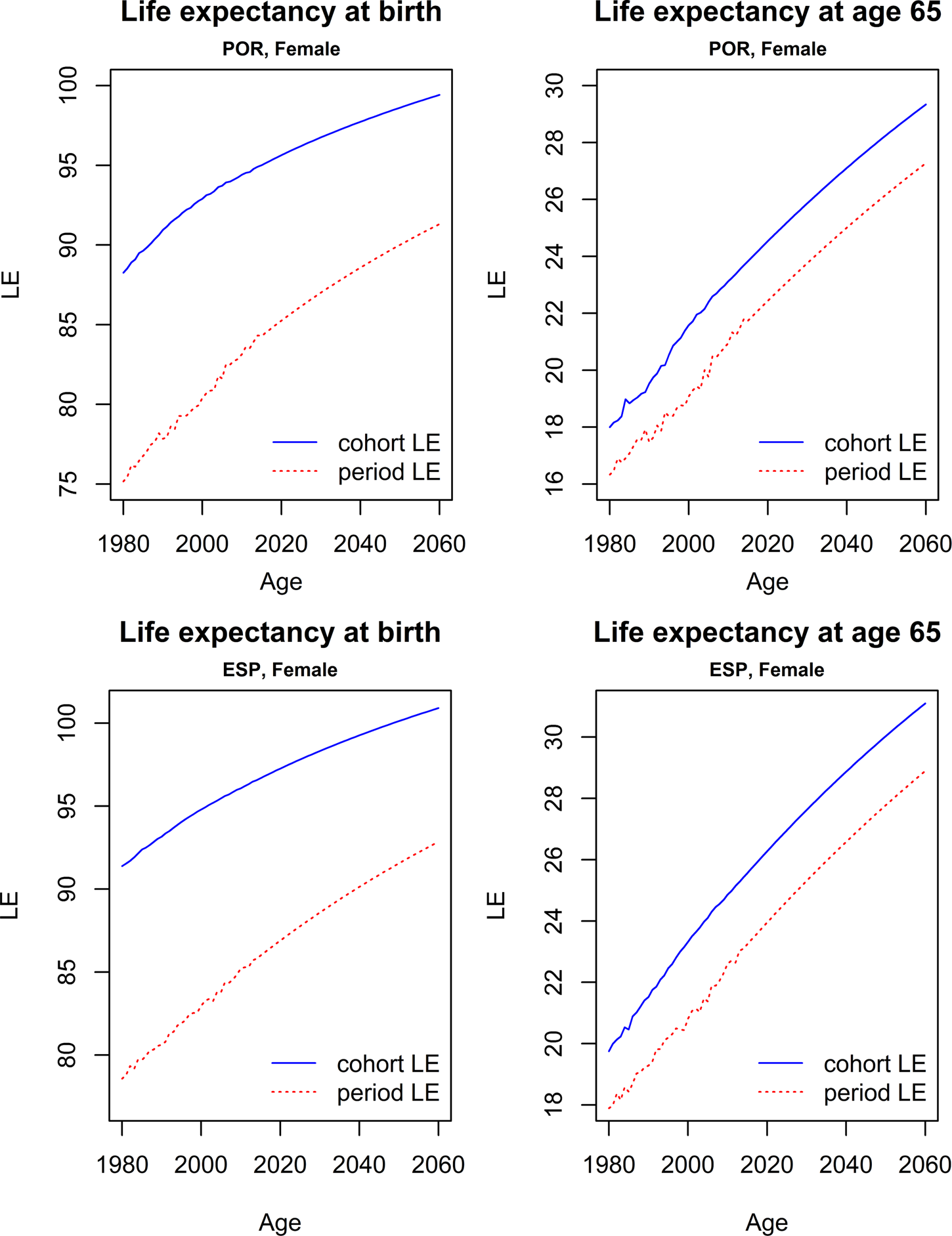
Figure 3. PLE and CLE for the Portuguese and Spanish female populations, 1980–2060.

Source: Authors’ estimates.

As is common in developed countries, average mortality rates are relatively high for newborns and children, then decrease rapidly toward their minimum (around age 12), increasing thereafter with age, reflecting higher mortality at older ages.Footnote ¹¹ The time trend parameter estimates k _t exhibit a clear decreasing tendency (approximately linear) in both countries, indicating the significant mortality improvements registered for all ages and both sexes over the last 35 years. The pace at which mortality improvements have taken place is not homogeneous across ages, however, as observed from the β _x parameter estimates. Observed mortality improvements have been more significant for youth, particularly in Portugal due to better infectious diseases control, better health care systems, and improved living conditions, but are also relevant for adults and the elderly. The forecasted mortality rates project into the future past trends observed in mortality across all ages (Figure 2). As can be observed, the Poisson-LC method projects a continued decline in mortality at these ages, with increased volatility around the general trend more significant at birth.

Figure 3 reports period and cohort life expectancies computed at birth and at age 65 for Portuguese and Spanish females for the period between 1980 and 2060. In both populations the life expectancy gap is significant, with PLE indicators clearly underestimating future longevity prospects. The difference is, as expected, more significant at birth (13.1 years in 1980 in Portugal and 12.8 years in Spain) than at age 65 (1.7 years in 1980 in Portugal and 1.9 years in Spain).Footnote ¹²

The life expectancy gap is expected to continue to be significant in both countries in the future, although the magnitude of $\dot{e}_x^{Gap} \lpar t_0{\rm \rpar \;}$is forecasted to decline at birth and to slightly increase at age 65.

4. Period versus cohort life expectancy estimates: international results

Cohort life expectancies currently exceed period life expectancies due to the observed decreases in mortality rates that started in the 18th century in some advanced countries and continue in the 21st century worldwide (see Ayuso et al., Reference Ayuso, Bravo and Holzmann2015). As explained in the preceding section, period tables are static tables built on the basis of the mortality behavior observed in the population during one period, while cohort tables incorporate projections of the future trend in mortality, taking into account observed changes over time, at birth and at different ages for different generations. The different demographic institutes across countries do not construct cohort tables as frequently as they do period tables. In fact, for most countries, information on observed and projected life expectancy based on static calculations (typically jointly collected for different countries by international organizations such as the UNFootnote ¹³, the World BankFootnote ¹⁴, EurostatFootnote ¹⁵, and OECDFootnote ¹⁶) can be found, and is systematically used in calculations related to pensions, health, long-term care, and welfare status; on the contrary, it is rare to find life expectancy estimates based on cohort tables.

This section compares the limited comparable country data on period and CLE that exist from official sources for Australia, the United Kingdom, and the United States, supplemented by the estimates of CLE for Portugal and Spain presented above.Footnote ¹⁷ The three data points cover the years 1981, 2010, and 2060. The period and CLE at birth and at age 65, by sex, and the corresponding life expectancy gap for these countries and selected calendar years are presented in Tables 1 and 2. The results for the analyzed countries at birth and at age 65 by sex are also plotted in Figures 4 and 5, respectively.

Figure 4. PLE and CLE at birth, by gender, 1980–2060.

Source: See Table 1. Note that the figure for Australia was directly reproduced from Productivity Commission (2013: 49).

Figure 5. PLE and CLE at age 65, by gender, 1980–2060.

Source: See Table 1. Note that the figure for Australia was directly reproduced from Productivity Commission (2013: 49).

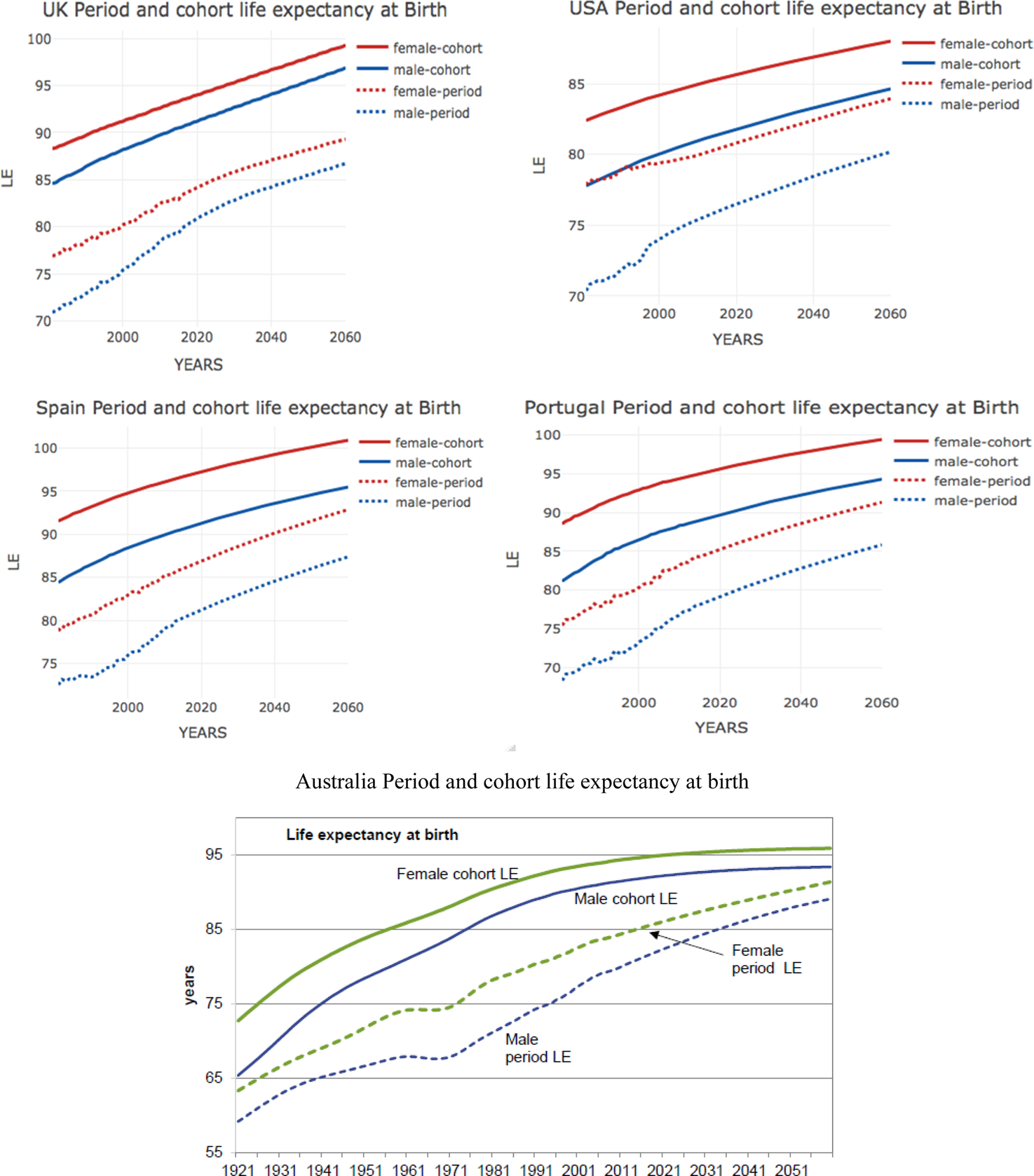
Table 1. PLE and CLE at birth, by gender: international comparison

Source: The United Kingdom (Office for National Statistics; 2014-based principal projection life expectancy variant); the United States (Life Tables for the United States Social Security Area 1900–2100); Australia (PCPOP and ABS 2008, Australian Historical Population Statistics, Cat. No. 3105.0.65.001; and ABS (various issues), Life Tables, States, Territories and Australia, Cat. No. 3302055001DO001); Spain (Period life expectancies – Instituto Nacional de Estadística INE; Cohort life expectancies – Authors’ estimates); Portugal (Period life expectancies – Instituto Nacional de Estatística INE; Cohort life expectancies – Authors’ estimates); $\dot{e}_0^{Gap}$ (author's calculations).

Note: All values expressed in years.

Table 2. PLE and CLE at age 65, by gender: International comparison

Notes: (1) For the UK, 1989 values; (2) For the UK, 2014 values; (3) For the UK, 2039 values. All values in years.

Source: The United Kingdom (Office for National Statistics; 2014-based principal projection life expectancy variant); the United States (Life Tables for the United States Social Security Area 1900–2100); Australia (PCPOP and ABS 2008, Australian Historical Population Statistics, Cat. No. 3105.0.65.001; and ABS (various issues), Life Tables, States, Territories and Australia, Cat. No. 3302055001DO001); Spain (Period life expectancies – Instituto Nacional de Estadística INE; Cohort life expectancies – Authors’ estimates); Portugal (Period life expectancies – Instituto Nacional de Estatística INE; Cohort life expectancies – Authors’ estimates); $\dot{e}_0^{Gap}$ (author's calculations).

Table 1 confirms that CLE estimates are always greater than those for PLE for all compared countries and years. These differences exceed 10 years for several countries and periods analyzed (e.g., 12.65 years for Australian men in 2010). This is the case for the United Kingdom, Australia, and Portugal, which have the greatest differences between the two estimates. Differences also exist in the United States and Spain, but are less pronounced (e.g., in the United States, the difference in life expectancy at birth between period and cohort estimates in 2010 is about 5.5 years). In all five countries, differences between the two values are projected to decrease over time, probably due to the smaller margin expected to improve survival probabilities (taking into account the high probabilities already reached in advanced ages).

Differences between countries are also observed by gender (Table 1, bottom panel). In general, greater differences are seen between the estimates of period and CLE at birth in men than in women. For instance, in 1981 the difference between the men and women life expectancy gap was 2.86 years in the United States and 4.44 years in Australia. Only in Australia is a greater difference projected for women in 2060, a phenomenon that also occurred in Portugal and Spain in 1981. However, a reduction in the differences between men and women is generally projected over time (except in Spain and Portugal, where they remain essentially unchanged), which could be driven by the reduction in the gender gap in life expectancy in these countries.

A similar analysis for life expectancy at age 65 is presented in Table 2. The results again show that estimated life expectancies from cohort tables are higher than those obtained from period tables in all five countries. The biggest life expectancy gap values are observed in Australia (up to an 11-year difference in life expectancy), followed by the United States (up to a 5-year difference). Again, projected values reflect a reduction in the (albeit still positive) differences between cohort and period estimates over time.

Analyzing the differences between men and women (Table 2, bottom panel), only small differences between genders tend to persist over time. In the United Kingdom, the United States, and Australia, men show greater differences between cohort and PLE estimates at 65 years; the opposite result is found in Spain and Portugal, which show slightly higher differences for women.

5. Implications for pension policy

Applying estimates of remaining life expectancy at retirement by using the lower PLE instead of the higher CLE has two key implications for pension policy.

First, at the individual level, doing so fails to establish an actuarially fair link between contributions and benefits, thus distorting individuals’ labor supply and saving decisions (contrary to the goal of recent reform attempts). Assuming that CLE is the correct estimate, using the lower PLE to calculate the initial benefit implies a subsidy for individuals that may not only bias one's labor supply while young and one's retirement decision when older – it may also affect one's saving and dis-saving decisions over a lifetime. While the bias can go in both directions, the income effect is likely to dominate the substitution effect, which may lower one's labor supply when young and advance the retirement age; for saving, one may lower accumulation efforts when young and decumulate faster when retired.

Second, at the pension scheme level, the use of the lower PLE makes the pension scheme financially unsustainable, as it incorrectly signals solvency; that is, that liabilities are smaller or at most equal to assets, while in reality this is not the case. This is valid for both unfunded and funded schemes: in funded schemes, assets are essentially unchanged by an underestimation of remaining life expectancy, while liabilities increase. In unfunded (nonfinancial) schemes, the contribution asset is negatively affected as it represents the present value of the difference between future contributions and the liabilities thereby created; if the life expectancies are actually higher, the pay-as-you-go (PAYG) asset must be lower and hence both liabilities and assets deteriorate, with liabilities higher and PAYG assets lower than assumed.

Of course, underestimation of actual life expectancy does not remain unnoticed, but emerges only gradually in periodic asset/liability checks or more often in the annual cash-flow comparison when expenditure due to longer periods of benefit payment exceed contribution revenues. The policy reaction is typically an ad hoc adjustment in nonfinancial defined benefit (NDB) schemes’ parameters (such as increasing the contribution rate, playing with the indexation parameters of benefits under disbursement, or calling for an increase in the retirement age; else the government transfers are increased). In nonfinancial defined contribution (NDC) schemes, the key policy options are a lower notional interest rate for the annual account accumulation and a lower indexation for benefits in disbursement. In both cases, the consequences of systematically underestimated life expectancy are shared in an ad hoc manner between the working and retired populations. Such a disruptive approach does not create the confidence in the scheme that pension economists consider important for a smooth and successful operation.

This section explores four policy areas: (a) How important is the difference between period and CLE for individual decisions and financial sustainability underestimation?; (b) What is the effect of the wrong life expectancy choice on the balancing mechanism recently implemented in a number of NDB and NDC schemes?; (c) If there is a difference between these schemes with regard to the choice of life expectancy estimation, what happens if heterogeneity in longevity exists?; and (d) How relevant are life expectancy changes as policy triggers after recent reforms?

6. How important is the difference between period and cohort life expectancy?

The fifth section offers the estimated magnitudes between period and cohort life expectancies at birth (age 0) and retirement (assumed at age 65). It is this latter age that matters most for pension policy considerations. Table 2 offers the scope of and differences between both approaches. These magnitudes and their ratio can be given a simple welfare economic interpretation through the concept of pension wealth (see Ayuso et al., Reference Ayuso, Bravo and Holzmann2017b). Pension wealth at any age is the present value of future benefit streams at this age. Assuming that the benefit indexation equals the discount rate (an assumption that broadly holds for wage-indexed pensions), then pension wealth at retirement is the pension benefit at retirement multiplied by life expectancy. If the scheme is actuarially fair, accumulation at retirement should equal pension wealth; that is, the devisor of the accumulation needs to be the correct life expectancy.

(14)$$PW_{65}\lpar t\rpar = b_{65}\lpar t\rpar \cdot \dot{e}_{65}\lpar t\rpar $$

(15)$$b_{65}\lpar t\rpar = AK_{65}\lpar t\rpar /\dot{e}_{65}\lpar t\rpar $$

(16)$$PW_{65}\lpar t\rpar = AK_{65}\lpar t\rpar \;{\rm for}\;{\rm an}\;{\rm actuarially}\;{\rm fair}\;{\rm scheme}$$

where PW ₆₅(t) is pension wealth, $\dot{e}_{65}\lpar t\rpar \;$life expectancy, AK ₆₅(t) accumulated contributions (plus interest), and b ₆₅(t) initial pension benefit, all at retirement age 65 in year t.

If the initial benefit is calculated by using the too-low PLE, then actual pension wealth exceeds the value of the accumulation by the ratio of the CLE to the PLE. Expressing the ratio as a change in the difference amounts to a subsidy that the generation would receive (unless corrective actions were undertaken).

(17)$${\rm Subsidy}\;{\rm rate\;} = {\rm \;}\displaystyle{{PW_{65}\lsqb {CLE} \rsqb } \over {PW_{65}\lsqb {PLE} \rsqb }}-{\rm \;}1{\rm \;} = \displaystyle{{\lpar {AK_{65}/\dot{e}_{65}^P } \rpar \times \dot{e}_{65}^C } \over {\lpar {AK_{65}/\dot{e}_{65}^P } \rpar \times \dot{e}_{65}^P }}-1{\rm \;} = \displaystyle{{\dot{e}_{65}^C } \over {\dot{e}_{65}^P }}{\rm \;}-{\rm \;}1$$

From Table 2, one can calculate the implicit subsidy rate at retirement that is behind the differences between period and CLE for the five countries and the 3 years of estimation (Table 3). The reason this can be called a subsidy rate is very simple: this is the rate at which own accumulations would need to increase to achieve the same benefit level as that derived from applying the PLE rate to own accumulations.

Table 3. Implicit subsidy rates of applying period over CLE at age 65 in select countries, by gender, 1981, 2010, and 2060

Source: Authors’ calculations based on Table 2.

Table 3 indicates both major differences and commonalities in the implicit subsidy rate between countries for which both period and cohort life expectancies are available. First, all countries have a declining relative gap between period and CLE and thus a shrinking subsidy. While for the age cohort of 1981 the average difference is 32% for men and 24% for women, the difference is projected to reduce to slightly above 10% for both genders for the age cohort of 2060. Second, the differences between genders are reduced across 1981, 2010, and 2060 for Australia, the United Kingdom, and the United States; in Portugal and Spain they remain broadly constant. Third, the differences between countries are also reduced. While the differences in 1981 between the highest and lowest country value were about 10:1, this ratio reduces to 2:1 in 2060.

It is not clear the extent to which these reduced differences are related to the application of similar or common estimation models or if these common trends actually constitute common underlying developments. In any case the scopes are relevant, and comparable in magnitude to the heterogeneity created by differences in lifetime income (see the fourth section). For the current mid-career generation of 1981 or the current primary school generation of 2010, the subsidy created by applying period instead of CLE is sizable and may distort their labor supply and saving decisions, working against the objectives of recent systemic and comprehensive parametric reforms in these five countries.

7. The balancing mechanism in defined benefit and defined contribution schemes

Most advanced and some emerging economies undertook systemic or comprehensive parametric reforms with the objective of making their pension system financially sustainable (or more specifically, their main earnings-related pension scheme(s)). To deal with future financial disequilibria, various countries introduced a balancing mechanism – that is, a rule-bound mechanism of parametric adjustments to the scheme that is triggered when financial disequilibria emerge.Footnote ¹⁸ The adjustment may be in the level of benefit indexation, a reduction in the nominal benefit level, a decrease in the annual accrual rate (in NDB schemes), or a change in the annual account indexation rate (in NDC schemes). What triggers the application of the balancing mechanism may simply be differences in expenditure and revenues of the scheme, or some measure of an actuarial imbalance based on the present value of deficits, or very rarely the application of more elaborate asset/liability comparisons. To establish financial (un-) soundness, some countries undertake annual or periodic actuarial assessments (such as Japan, Sweden, the United Kingdom, and the United States).

How are these balancing mechanisms influenced if the ‘wrong’ mortality/life expectancy data are selected? What is the scope of underestimated liabilities? Are assets also affected? Is there a difference between benefit type (DB/DC) and funding mechanism? These issues are discussed next in turn.

8. Adding heterogeneity considerations to estimation of life expectancy

For pension schemes the issue of correct estimation of future life expectancy of a retiree cohort is complicated by the increasing recognition that this mean estimate has a dispersion that is linked to the level of lifetime income and accumulated savings (Ayuso et al., Reference Ayuso, Bravo and Holzmann2017a, Reference Ayuso, Bravo and Holzmann2017b). Hence, not taking account of both issues may lead to multiple and interrelated distortions at both the individual and scheme level.

For example, the wrong mean estimate for life expectancy leads to underestimation of the pension scheme's liability. If the same common life expectancy is applied to all cohort members at retirement, a second underestimation of the liability is introduced, as richer individuals have a higher life expectancy. For the highest income decile, the individual subsidy rate may reach 30% for women and 15% for men. In contrast, those in the lowest income decile may face a tax rate of 20% or more on a much lower pension. The scope of the aggregate underestimation of liabilities will depend on the distributive characteristics and choice of the mean value (average or median), but is hypothesized to be 10–15%.

The interaction of both effects on individuals and their labor supply and saving decisions has not yet been worked out. For lower-income groups, the tax rate effect of heterogeneity is counteracted by an incorrect lower mean value. For higher-income groups, the subsidy effect of heterogeneity is fortified by the subsidy effect of a too-low mean estimate. How this affects individuals’ decisions will also depend on their perceptions of their own life expectancy. Understanding these mechanisms is important for designing appropriate policy interventions. For correct mean and heterogeneity estimates, the effectiveness of some policy proposals has already been estimated (Holzmann et al., Reference Holzmann, Alonso-García, Labit-Hardy, Villegas, Holzmann, Palmer, Palacios and Sacchi2019).

9. Life expectancy measures in recent pension reforms

In recent decades, most OECD countries responded to continuous growth in life expectancy with pension reforms in which a common feature is to create an automatic link between future pensions and changes in life expectancy. The link between life expectancy and pension benefits has been accomplished in at least six different ways (Whitehouse, Reference Whitehouse2007; OECD, 2017):

• • By introducing FDC plans as a (often partial) replacement for unreformed NDB pensions (e.g., Mexico, Poland, Sweden);

• • By introducing an automatic link between life expectancy and pension benefits, for example through demographic sustainability factors (e.g., Finland, Portugal, Spain);

• • By linking the normal retirement age to life expectancy (so far 10 countries including Denmark, Italy, the Netherlands, and Portugal);

• • By connecting years of contributions needed for a full pension to life expectancy (e.g., France);

• • By substituting traditional NDB public schemes with NDC schemes that replicate some of the features of FDC plans, namely the way in which pension (annuity) benefits are computed (e.g., Sweden, Poland, Latvia, Italy, Norway);

• • By linking penalties (bonuses) for early (late) retirement to years of contributions and normal retirement age (e.g., Portugal).

These reforms represent a fundamental change in the way longevity risk is shared between contributors and retirees, and between current and future generations, that has become more explicit and, in principle, based on automatic rules rather than ad hoc changes as in the past. However, the legislated automaticity in countries must still stand the test of time. And even if automatically introduced and moving in the right direction, these measures are almost always incomplete and insufficient to assure financial sustainability issues triggered by life expectancy changes. This adds to issues of not selecting the correct life expectancy under these mechanisms and the incentive distortions involved.

In almost all cases and countries, the PLE measure has been used to link longevity and pension benefits, which, as discussed above, results in underestimating remaining lifetime at retirement. This option has consequences on the way longevity risk is shared between generations. The financial consequences of underestimating life expectancy during retirement are ultimately borne by those who fund the pension scheme; that is, younger cohorts in NDB/NDC schemes and private contributors/sponsors in FDB/FDC schemes.

For instance, demographic sustainability factors introduced in Finland, Portugal, and Spain automatically link initial pension benefits to life expectancy observed at the time of retirement, leading, in most cases, to a reduction in pension entitlements. These sustainability factors are computed as a simple ratio between period life expectancy observed at some reference age (e.g., 65 in Portugal and 67 in Spain) in some (past) reference year (e.g., 2000 in Portugal and 2012 in Spain) and period life expectancy observed at the time of retirement (in Spain according to mortality tables for the pensioner population as they are designed by the social security system). By design, these sustainability factors are not consistent with an actuarially neutral pension scheme since they do not guarantee that by adjusting (reducing) initial pension benefits but paying them for a longer period the scheme is financially neutral. To the extent that trends in period and cohort life expectancies differ between past and current generations, the system could redistribute in favor of older cohorts and have a negative impact on the public pension system's sustainability.

Linking the normal retirement age to period life expectancy instead of CLE will extend working lives but will be insufficient to preserve actuarial neutrality between contributions and benefits, thus maintaining major distortions in individual labor supply and saving decisions, and forgoing the macroeconomic impact of higher levels of employment on investment, gross domestic product, consumption, and public finances. Moreover, the lower-than-consistent-with-actuarial-neutrality increase in the retirement age reduces the size of the positive effect on pension adequacy resulting from longer contribution careers and higher pension accruals.

Linking penalties (bonuses) for early (late) retirement to years of contributions and normal retirement age using period life expectancy measures does not ensure actuarial neutrality between contributions and benefits. Actuarial neutrality depends on the parameters that determine the annuity factor – survival probabilities, indexation rate, discount rate – that revert to life expectancy when the indexation rate equals the discount rate. Increases in life expectancy require higher penalties for early retirement and lower bonuses for late retirement to keep up with actuarial neutrality. Adopting a period approach in measuring life expectancy to assess the work incentives around retirement ages systematically underestimates the magnitude of the penalties (bonuses) for early (late) retirement needed to ensure actuarial neutrality and a fair share of longevity risk between generations, and is likely to reduce labor supply.