2.0 COMPUTATIONAL METHODOLOGY: HMB3

For this investigation, the in-house CFD solver HMB3 is used. The core functionality of HMB3 is CFD, however its use has been extended in recent years to include whole engineering applications, including helicopter rotor aeroelasticity^{(Reference Dehaeze and Barakos12)} and propeller validation^{(Reference Chirico, Barakos and Bown13,Reference Barakos and Johnson14)} . In addition to this, the time-marching aeroelastic method of HMB3 has been validated with respect to propeller stall flutter for the Commander propeller blade^{(Reference Higgins, Jimenez-Garcia, Barakos and Bown15,Reference Higgins, Jimenez-Garcia, Barakos and Bown16)} .

2.1 Computational fluid dynamics

Previous investigations using HMB3 have provided propeller flow validation in both installed and isolated conditions, by comparison with the experimental results of the JORP propeller^{(Reference Scrase and Maina17)} and the IMPACTA wind-tunnel tests^{(Reference Gomariz-Sancha, Maina and Peace18,Reference Knepper and Bown19)} . Good agreement was found in terms of aerodynamics and acoustics^{(Reference Barakos and Johnson14,Reference Chirico, Barakos and Bown13)} . HMB3 solves the Navier-Stokes equations in integral form and are discretised using a cell-centered finite volume approach on a multi-block grid. The spatial discretisation of these equations leads to a set of ordinary differential equations in time,

(1) \begin{equation} \frac{d}{dt} ({\bf W}_{i,j,k} V_{i,j,k}) = - {\bf R}_{i,j,k} ({\bf w}),\end{equation}

where i, j, k represent the cell index, W and R are the vector of conservative variables and flux residual respectively and $V_{i,j,k}$ is the volume of the cell i,j,k. Greater detail on the numerical techniques employed can be found within the previous investigations conducted using HMB3^{(Reference Dehaeze and Barakos12,Reference Chirico, Barakos and Bown13,Reference Barakos and Johnson14,Reference Barakos, Steijl, Badcock and Brocklehurst20,Reference Steijl, Barakos and Badcock21,Reference Lawson, Woodgate, Steijl and Barakos22,Reference Crozon, Steijl and Barakos23,Reference Babu, Loupy, Dehaeze, Barakos and Taylor24)} . Several turbulence models, of both URANS and hybrid LES/URANS families, are available in the HMB3 solver. For this investigation the standard $k-\omega$ turbulence model will be compared to the hybrid LES/URANS method known as Scale Adaptive Simulation (SAS)^{(Reference Menter and Egorov26,Reference Menter and Egorov27)} . The SAS formulation allows for the dynamic adjustment of the von Karman length scale to produce an LES-like solution. HMB3 SAS simulations have been conducted in the past focusing on transonic cavity flows^{(Reference Babu, Zografakis, Barakos and Kusyumov25)} and missile projection^{(Reference Loupy, Barakos and Taylor28)}. Because this investigation requires the deformation and relative motion of the propeller blade, in order to achieve this, the chimera method is used^{(Reference Jarkowski, Woodgate, Barakos and Rokicki29)}. ICEM-Hexa^TM of ANSYS is used to generate all structured grids for this investigation.

2.2 Computational structural dynamics

The aeroelastic framework of HMB3 is based on the modal method^{(Reference Higgins, Jimenez-Garcia, Barakos and Bown16,Reference Babu, Loupy, Dehaeze, Barakos and Taylor24)} . This method uses externally computed structural modes and a mesh deformation module based on the inverse distance weighting interpolation. The modal approach was selected in order to reduce computational cost as it expresses solid deformations as functions of the structure’s eigenmodes.

A NASTRAN finite element model is created in order to obtain the structural mode shapes and frequencies. The finite element model uses non-linear PBEAM elements to model the structure’s mass and inertia distribution along the span, with rigid bars (RBAR) elements used to connect the PBEAM node to each of the fluid mesh points at the given section. A non-linear static analysis (SOL 106) is computed to obtain the mode shapes and frequencies, along with a static deformation to rigid loads.

At the beginning of each computation, the structural modes are interpolated from the CSD to the CFD grid. The interpolation is performed with the Moving Least Square method (MLS). The MLS method allows for sufficient accuracy in terms of the modal force and displacement estimations due to the fact these values are calculated based upon the CFD grid without further interpolation to the CSD.

3.0 TWO-DIMENSIONAL AERODYNAMIC DAMPING

Very few 2D cases have been computed for specific propeller sections to allow for the introduction of the SAS approach for the calculation of aerodynamic damping. As a result, the NACA 0012 section was selected due to the amount of experiment data available at different pitching conditions. The $70\% R$ and $90\%R$ Commander aerofoils were also investigated to provide a comparison with the NACA 0012 for a specific propeller section.

3.1 2D aerodynamic damping calculation

To fully determine the stability of the aerofoil section, the amount of aerodynamic damping within the system can be computed via the integration of the pitching moment coefficient with respect to the pitching angle. Such a method was described by Corke in 2015^{(Reference Corke and Thomas30)} with the derivation of the aerodynamic damping shown in Equation 2, where $C_m^D$ and $C_m^U$ are the pitching moment coefficients on the downstroke and upstroke, respectively, and $\alpha_h$ is the harmonic pitching angle.

(2) \begin{equation} \theta_{cycle} = \frac{1}{\pi \alpha_h^2} \int \left( C_m^D - C_m^U \right) d \alpha\end{equation}

3.2 Computational setup

3.2.1 NACA 0012 section

The topology of the grid follows a traditional C-grid type with a downstream far-field boundary applied at 15 chords from the trailing edge. In terms of the mesh, 650 cells were distributed around the aerofoil with 85 cells distributed via an exponential law, clustering to $1\times 10^{-6}\ C_{ref}$ , outward of the aerofoil surface.

Standard two-dimensional boundary conditions were applied to the spanwise boundary faces for an initial verification of the mesh quality and CFD setup, with a single computational cell in the spanwise direction of length 1 chord. A single chord spanwise length was selected due to the ease of non-dimensional load scaling within HMB3. Following this, the two-dimensional conditions were replaced with periodic boundary conditions. This allows for quasi-3D simulations where scale-resolving turbulence modelling can be implemented. For this investigation standard URANS closed with the $k-\omega$ shear-stress-transport (SST) turbulence model was compared to SST-SAS. No difference in aerofoil loads was observed between the 2D and quasi-3D simulations using the standard URANS formulation, hence, only the 2D URANS loads are presented. For the quasi-3D simulations, the spanwise length was set to a quarter of the chord. A quarter chord is selected based upon the findings of the LESFOIL project^{(Reference Mellen, Fröhlich and Rodi31)}. For accurate turbulence production from scale-resolving methods, the spanwise extend of the aerofoil must not be greater than a quarter of the chord.

The test conditions for this calculation are presented in Table 1 and correspond to experiments by McAlister in 1982^{(Reference McAlister, Pucci, McCroskey and Carr1)}. These test conditions were selected as they represent typical flow conditions found during the dynamic stall of a helicopter rotor in forward flight and based upon the experimental report, these test conditions were found to have negative aerodynamic damping.

Table 1 Test conditions for the dynamic stall computations

3.3 NACA 0012 quasi-3D results

Presented in Fig. 2 is the pitching moment coefficient results for the NACA 0012 test case, comparing 2D URANS and phase-averaged quasi-3D SAS, to experiments.

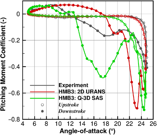
Figure 2. Comparison of the NACA 0012 pitching moment coefficient for the 2D and quasi-3D simulations to the experiment, with the flow conditions presented in Table 1.

In the experimental results, the pitching moment remains almost constant up until $22^{\circ}$ , where it starts to increase, with the peak pitching moment coefficient observed at the maximum angle of $25^{\circ}$ . A similar response is found with the 2D URANS simulation, however, the peak pitching moment is found to be greater. Based upon the 2D URANS results, this response is seen to be based upon the development of stalled flow across the aerofoil trailing edge. This is observed in the flow visualisation results of Fig. 3(a,c,e). The negative pitching moment for the quasi-3D SAS simulation is found to increase earlier at $18^{\circ}$ , and this correlates with an increase in the developed detached flow. Fig. 3(b,d,f) highlight the earlier development of detached flow, particularly at $22^{\circ}$ where the stalled flow is seen to be further upstream towards the leading-edge for the quasi-3D SAS result in comparison to the 2D URANS.

Figure 3. Flow visualisation of $|\hat{\omega}|=[1.0,5.0,10.0]$ iso-surfaces during the aerofoil upstroke.

The recovery of the pitching moment during the experiment is found to occur over a range of $13^{\circ}$ , eventually recovering and crossing the upstroke profile around $12^{\circ}$ . During the downstroke, the 2D URANS is found to have a significant secondary stall event, resulting in two pitching moment peaks. The 2D URANS then quickly recovers, crossing the upstroke profile $6^{\circ}$ earlier than experiments at $18^{\circ}$ . This indicates that the 2D URANS simulation develops a closed stall bubble. This sheds from the section quickly, allowing the flow to attach at an earlier pitch angle than seen during the experiment. This is observed in the flow-field visualisation results for the URANS simulation in Fig. 4(a,c,e). For the quasi-3D SAS, following the peak, the pitching moment recovers to similar values as the experiment. The experimental pitching moment, during the downstroke, is seen to increase around $18^{\circ}$ . This indicates the development of further separated flow between the $22^{\circ}-18^{\circ}$ range, as observed in Fig. 4(b,d,f). This is also present in the quasi-3D SAS simulation, however, the magnitude of this secondary event is found to be larger. The quasi-3D SAS simulation then begins to recover crossing the upstroke profile at the same angle as experiments. An average variation of $\pm 0.5^{\circ}$ is found for the recovery angle, thus resulting in the closer estimation to the experimental recovery angle for the phased-averaged quasi-3D SAS than the 2D URANS simulations.

Table 2 NACA 0012 aerodynamic damping

This variation in recovery angle is the result of cycle-to-cycle differences in the pitching moment coefficient for the quasi-3D SAS simulation. Cycle-to-cycle variations in dynamic stall experimental data has been discussed recently by Ramasamy et al.^{(Reference Ramasamy, Sanayei, Wilson, Martin, Harms, Nikoueeyan and Naughton32)}. They analysed two sets of experimental data and found that traditional phase-average filtering is not effective enough to represent dynamic stall load measurements. As a result, two new data-driven algorithms were developed to cluster the load results based upon the developed flow phenomena. Significant differences were found in the aerodynamic damping and load results between the two new clusters and the traditional phased-averaged solutions. From this study it is clear that an improvement in the analysis of experimental results is required to ensure the correct flow physics is captured.

Using the pitching moment curve, the aerodynamic damping of the system is estimated and presented in Table 2. As expected from the experimental report, a negative damping value is seen for both 2D URANS and quasi-3D SAS simulations. However, due to the sharp recovery of the 2D URANS simulation, the positive anti-clockwise moment loop is greater than seen from the experiment, therefore the damping estimation is below the experiment. The quasi-3D SAS simulation provides a larger negative damping value for the phased average solution, at a closer percentage to the experiment than the 2D URANS. In addition, a scatter in the estimated aerodynamic damping of $\pm37\%$ is observed per revolution, thus resulting in a closer estimation to the experimental results.

Figure 4. Flow visualisation of $|\hat{\omega}|=[1.0,5.0,10.0]$ iso-surfaces during the aerofoil downstroke.

One of the objectives of this investigation was to determine which method, 2D URANS or quasi-3D SAS, best captures the characteristics associated with stall flutter. Based upon the aerodynamic loads, the 2D URANS performs better during the upstroke with the pitching moment coefficient increasing at the same position as the experiment. However, it is the downstroke segment of the oscillation that has the greatest effect on the level of aerodynamic damping due to the amount of unsteady flow features present during this stage. On this basis, the quasi-3D SAS simulation performs better as the levels of aerodynamic damping better represent what was seen in the experiment. Overall, neither URANS or SAS are perfect for dynamic stall predictions, though the SAS appears to be better in representing the separated flow and this is important in the present investigation.

3.4 Commander aerofoil 2D aerodynamic damping estimation

3.4.1 70% radial station

Presented in Fig. 5(a) is the pitching moment coefficient of the Commander propeller section of the 70% radial station. As can be seen from the 2D URANS simulation results, a stable pitching moment profile is derived. During the upstroke, an almost constant negative pitching moment of $-0.1$ is seen up until $15^{\circ}$ . Following this, the aerofoil section separates causing the increase in negative pitching moment. Following the shedding of the developed closed stall bubble, the pitching moment recovers within $1^{\circ}$ . As a result of this sharp recovery, the pitching moment loops do not cross, and hence, a stable anti-clockwise loop is derived.

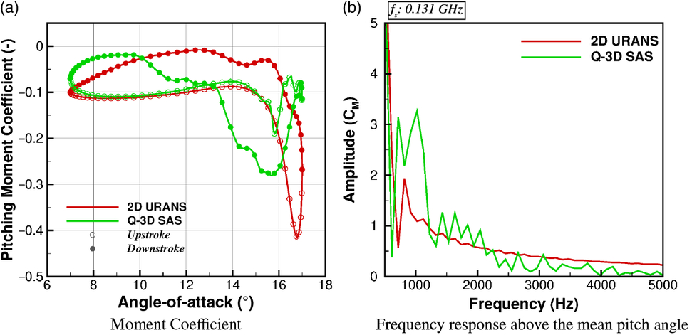
Figure 5. Pitching moment response of the $70\%R$ Commander aerofoil section.

For the quasi-3D SAS simulation, similar values of pitching moment are found during the upstroke, with the same stall angle of $15^{\circ}$ . Following the initial stall, the detached flow is shed resulting in a small recovery/reattachment of the flow-field. As the angle-of-attack is increased further, detached flow again develops and vortices are shed from the aerofoil, accumulating during the peak pitching moment. The quasi-3D SAS simulation recovers around $12^{\circ}$ . Due to this initial recovery on the upstroke, a negative clockwise moment loop is derived, resulting in negative aerodynamic damping, as shown in Table 3. The 2D URANS shows a stable solution.

A Fast-Fourier-Transform was conducted on the pitching moment coefficient results above the mean angle-of-attack of $12^{\circ}$ , with the results presented in Fig. 5(b). For these simulations, a sampling frequency of $0.131$ GHz is used, thus resulting in a maximum available frequency of $0.066$ GHz. The Nyquist theorem is therefore satisfied for these comparisons. For the 2D URANS result, a single peak at 1kHz is found and this corresponds to the peak moment coefficient. A similar peak is found in the quasi-3D SAS simulation, however, due to the double stall event, a double peak is observed from the frequency response with the frequency band ranging from $0.7$ to $1.4$ kHz. At higher frequencies, several oscillations from the quasi-3D SAS simulation are observed. This is expected to due to the resolution of scales not captured via URANS and the oscillations in pitching moment coefficient seen at the maximum pitch angle. Some small oscillations are present at higher frequencies for the 2D URANS case, however, these are negligible in comparison to the quasi-3D SAS response.

Table 3 $70\%R$ aerodynamic damping

3.4.2 90% radial station

Similar responses are found between the 2D URANS and quasi-3D SAS simulations. A full anti-clockwise moment loop is found, and presented, in Fig. 6(a) for the 2D URANS simulation. The pitching moment begins to increase around $11^{\circ}$ . This is $3^{\circ}$ above the mean angle-of-attack. The pitching moment recovers almost instantly resulting in a stable moment loop.

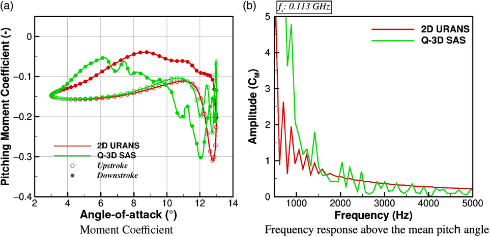
Figure 6. Pitching moment response of the $90\%R$ Commander aerofoil section.

In a similar manner to the 70% station, after the pitching moment begins to increase, and the detached flow develops, the flow-field is shed from the station resulting in a recovery of the pitching moment for the quasi-3D SAS simulation. Several vortices from the detached flow are shed and this gives oscillating pitching moment as the section reaches the maximum angle-of-attack. During the downstroke, the pitching moment increases producing an unstable clockwise moment loop. The pitching moment recovers around the mean angle-of-attack. The resultant anti-clockwise moment loop causes a reduction in the aerodynamic damping, presented in Table 4.

Table 4 Aerodynamic damping

The frequency response for the pitching moment curve above the mean angle-of-attack of $8^{\circ}$ is presented in Fig. 6(b). The sampling frequency was reduced to $0.113$ GHz due to the increase in sample time-step. This sampling frequency still satisfies the Nyquist theorem in order for a comparison to be made. For the 2D URANS simulation, several peaks are observed below 1kHz, with the highest amplitude seen at $0.6$ kHz. The quasi-3D SAS simulation produces a two high amplitude peaks at $0.75$ and $1.2$ kHz, corresponding to the two stall events.

3.5 Summary of the two-dimensional aerodynamic damping investigation

It is concluded that the use of the SAS method provides a more realistic representation of the negative aerodynamic damping associated with stall flutter, as seen from the NACA 0012 damping estimations. Therefore, to conduct a stall flutter investigation, it is vital that scale-resolving aerodynamics are used which captures the fluctuations in surface pressure associated with vortex shedding.

4.0 THREE-DIMENSIONAL AERODYNAMIC DAMPING

Using the derived time-marching aeroelastic method, the Commander blade is modelled in isolation. This test case was selected due to the high torsional response seen in tests^{(Reference Burton5)}. During model implementation, simulations were conducted utilising the full propeller, nacelle, wing combination, however, due to the large computational cost associated with such a simulation, and due to the fact that it is the detached flow associated with the reference blade that triggers the aeroelastic excitation (the excitation is then propagated to the additional blades via the nacelle connection with a phase difference seen within the excitation between blades), periodicity in space is assumed. This allows for the reduction of the computational domain to one propeller blade.

The baseline propeller design consisted of three blades, with an aspect ratio of $\sim\,11.0$ , and reference tip chord of $\sim\,0.13$ m.

4.1 3D aerodynamic damping calculation

To determine the stability of the propeller blade, the amount of aerodynamic work (W) can be used. This involves the integration of the unsteady surface pressure $ (\tilde{p}) $ and local displacement velocity $ (\vec{u}) $ over time (Equation 3). A test case which has a negative aerodynamic damping value, i.e. a destabilising flow, will have positive aerodynamic work. This method is used to determine the stability of the entire blade.

(3) \begin{equation}{W = \int \left( \tilde{p} \cdot (\vec{u} \cdot \vec{n}) \right) d\tau}\end{equation}

To relate the three-dimensional calculation to the two-dimensional aerofoils, as per the two-dimensional aerofoil calculations, the moment curve of a propeller blade section is used to determine the stability of the section. For the two-dimensional calculations, a sinusoidal rigid motion is applied to the aerofoil and this determines the change in angle-of-attack. For a full three-dimensional aeroelastic simulation, a test case which is active in torsion is required to obtain this change in angle-of-attack for the estimation of the aerodynamic damping coefficient.

Due to the employed multi-block mesh, selected block faces along the propeller blade surface can be used to determine the current pitch angle and pitching moment. The instantaneous pitch angle is calculated based upon reference leading-edge and trailing-edge node positions from the rigid blade. Presented in Fig. 7 are the selected block faces for the Commander propeller blade from the 50% to 90% radial station. For this investigation, and as per the dynamic stall study, focus will remain on the 70% and 90% radial stations.

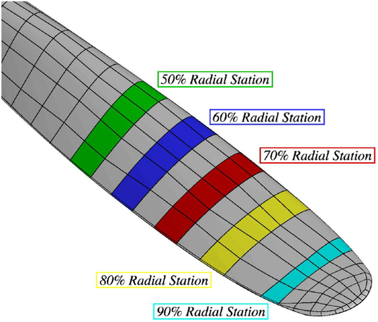
Figure 7. Commander propeller sections used for the damping calculations.

Based upon the derived pitching moment and pitch angle, the aerodynamic damping is estimated via Equation 4:

(4) \begin{equation}\theta_{cycle} = \int \left( C_m^{D*} - C_m^{U*} \right) \partial \alpha,\end{equation}

where $C_m^{D*}$ and $C_m^{U*}$ are the pitching moment coefficients along the radial station minus the mean value observed for that section, with superscripts ^D and ^U indicating downstroke and upstroke, respectively. To determine the aerodynamic damping based upon a change in pitching moment, and therefore relate such aerodynamic damping estimations to the two-dimensional study, the mean value of the pitching moment is subtracted from the instantaneous to ensure the blade rotational effects become less influential.

4.2 Computational setup

Based upon the supplied geometry a computation domain of $120^{\circ}$ was created with a radial distance from the origin of $5\ R/c$ . The inflow was selected to be also $5\ R/c$ with the outflow $8\ R/c$ from the origin in the vertical direction, this is shown in Fig. 8(b). A solid cylindrical hub was created to simplify the background topology with the hub extending the length of the computational domain, from inflow to outflow.

A chimera grid (Fig. 8a) was used to allow for the deflection of the blade during the aeroelastic computations. A C-O-grid was used for the foreground mesh, and this was due to the blunt trailing edge and blade tip design. The blade root section was cut at $0.124\frac{r}{R}$ . This station was selected to remove the need to mesh around the complex hub mounting structures and also ensure a sufficient amount of cells are placed radially inwards for the chimera interpolation. A conventional background grid was derived for the computational domain. A grid convergence study was conducted with the grid sizes presented in Table 5.

Table 5 Grids used for mesh convergence study of the 3D aeroelastic cases

The baseline test conditions for this propeller were based upon the initial starting conditions of the static wind-tunnel test conducted by DOWTY in the 1970s^{(Reference Burton5)}. Sea-level conditions were assumed, with the reference velocity and length, for the Reynolds number, selected as the tip Mach number at 1400(rpm) and tip chord length, respectively. Following the convergence of the rigid flow-field at 1400(rpm), the aeroelastic method was then used^{(Reference Higgins, Jimenez-Garcia, Barakos and Bown15)}.

A single revolution is used to settle the structural response. Following this, the blade rotational velocity was accelerated from 1400 to 1750(rpm) over 5 revolutions. This acceleration mirrored the process conducted during the experiment. Table 6 details the computational parameters.

Table 6 Summary of the Commander propeller blade test conditions

A time-step comparison is conducted using 1^◦ and 0.5^◦ steps per propeller revolution.

4.2.1 Structural modelling

For the aeroelastic simulation, a NASTRAN structural model is derived to obtain the mode shapes and frequencies for the modal aeroelastic method. The structural model for the Commander blades are based upon the assumption of a solid material blade. The linear mass distribution is calculated as a function of the cross-section area, with the blade inertia based upon the integration of the aerofoil section shape. The blade was assumed to be of 1100 grade aluminum alloy, resulting in a Young’s Modulus of 69GPa, Shear Modulus of 26GPa and mass density of 2710kg/m $^3$ . The cross-sectional area, linear mass and blade sectional inertias are presented in Fig. 9(a). The derived mode shapes match those seen within the experiment, with Fig. 9(b) showing the frequency response compared to the experiment.

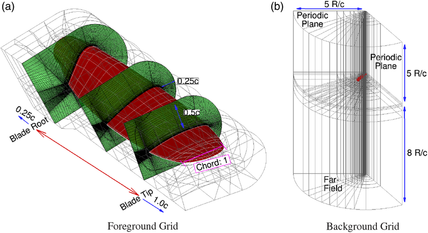
Figure 8. Commander propeller computational domain and chimera grid.

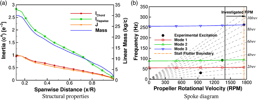
Figure 9. Commander propeller blade structural properties and resultant spoke diagram.

In terms of structural damping, a value is supplied to the modal method. For these calculations a transition was made from an initial high value of 0.10 to a final value of 0.001. This allows for the control of the initial aeroelastic response during the first aeroelastic revolution.

4.3 Commander propeller blade 3D aerodynamic damping estimation

Presented in Table 7 is the aerodynamic damping estimation from the 3D aeroelastic test case for the URANS and SAS simulations. As can be seen, and as expected from the dynamic stall study, positive damping values are observed for the URANS results, with reduced damping estimations seen for the SAS. At the 70% station, the damping estimation reduces by 50%, with the 90% station reducing further producing a negative damping estimation. This reduction in aerodynamic damping for the SAS result is also found within the amount of aerodynamic work derived from the entire blade. As observed from Table 7, the URANS result produces a negative work estimation with the SAS solution producing positive work. From experimental^{(Reference Burton5)} and simulation data^{(Reference Higgins, Jimenez-Garcia, Barakos and Bown15)}, it is known that this propeller blade is found to suffer from stall flutter. Analysis of the modal amplitudes from the simulation data found the SAS results to significantly increase in torsional content with the trend in terms of torsional stress observed across the blade. This is presented in Fig. 10. Through the use of the SAS method, the negative aerodynamic damping value associated with stall flutter is achieved.

Table 7 Comparison three-dimensional aerodynamic damping estimates for the 3D URANS and SAS simulations over the entire simulation

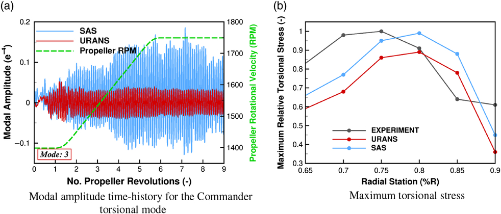
Figure 10. Time history of the modal amplitude results and torsional stress trends across the blade for the aeroelastic validation^{(Reference Higgins, Jimenez-Garcia, Barakos and Bown16)}.

As previously stated, the 3D aerodynamic damping is estimated using the changes in pitching moment. This is presented in Fig. 11 for the 70% and 90% radial stations. As observed from both URANS and SAS simulations, there is a significant shift in pitching moment at the start of the first revolution. This is a result of the start-up of the aeroelastic deformations. Following this, oscillations in both URANS and SAS simulations settle, with a linear increase in the pitching moment found during the transition phase for both radial stations. Examining the profiles for the 70% station, an order of magnitude larger variations in pitching moment are observed during the transition phase for the SAS simulation when compared to the URANS. This increases to two orders of magnitude following the completion of the acceleration. For the 90% station, a linear trend in pitching moment is also observed during the transition for the URANS and SAS simulations, however, once the acceleration is complete, significant fluctuations of $\pm 0.4$ in $C_m$ , are captured by the SAS.

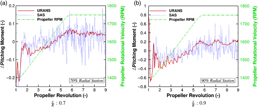
Figure 11. Comparison of the change in pitching moment for the URANS and SAS simulations.

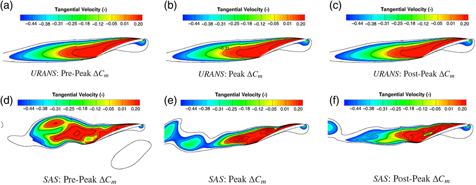
Figure 12. Flow visualisation at $\frac{x}{R}: 0.9$ of the tangential velocity profile for the SAS and URANS simulations at maximum $\Delta C_m$ .

Shown in Fig. 12 is the flow visualisation, using radial slices, of the non-dimensional tangential velocity at the 90% radial station around the maximum change in pitching moment for the URANS (a,b,c) and SAS (d,e,f) simulations. The tangential velocity is the dominant component across the aerofoil section, therefore, its fluctuations highlight the alterations in detached flow. As can be seen from both the URANS and SAS results, the 90% station is fully stalled. This results in an entire stall bubble predicted by URANS. Very slight changes are observed around the peak value for the URANS simulation, in which the detached flow moves towards the leading-edge, thus changing the pressure distribution. The change in pressure distribution on the upper surface, for the URANS simulation, is shown in Fig. 13(a). There is a reduction in pressure towards the leading-edge at the peak moment location due to the increase in the stalled flow. This detached flow then travels further downstream causing an increase in pressure which reduces the pitching moment. These changes in surface pressure coefficient, and hence pitching moment, for the URANS simulations are small in comparison to the SAS.

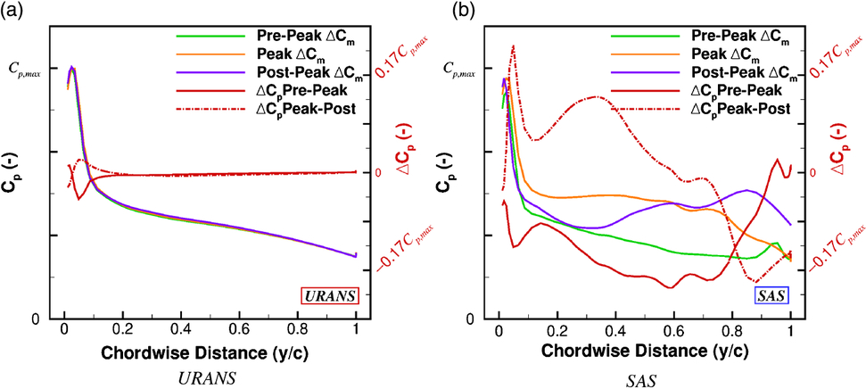
Figure 13. Surface pressure coefficient on the blade upper surface at the 90% radial station through the peak $\Delta C_m$ for the URANS and SAS simulations.

Looking at the SAS flow visualisation results, the structure of the detached flow is significantly different when compared to the URANS. For the URANS, one singular vortex is produced, whereas the SAS method is able to capture the smaller vortex structures which combine to create the entire section wake. Looking at the pre-peak station (Fig. 12(d)), at least five vortical structures can be observed for the SAS result. There are three small pockets of detached flow on the blade surface, with two larger structures beginning to shed. As peak pitching moment is reached (Fig. 12(e)), the two larger vortices have shed from the station. This shedding causes a significant reduction in pressure, as observed from Fig. 13(b). Following the shedding of the two larger vortices, the flow attempts to recover post-peak resulting in a positive shift in pressure. It is this process of vortex shedding which causes the larger fluctuations in pitching moment and hence reduced stability in terms of the aerodynamic damping.

To summarise, using the change in pitching moment from its mean and the aeroelastic blade pitch angle, the aerodynamic damping of a given propeller section can be estimated. A comparison of the aerodynamic damping is made of the Commander propeller blade, which is found to be active in torsion, using URANS and SAS methods. Both observed radial stations, with the SAS simulation were found to produce lower levels of aerodynamic damping. This is due to the fact that greater amounts of flow features, such as shedding open stall bubbles, are produced, and therefore cause greater variation in loads and blade deflections. This correlates to the dynamic stall investigations in which the aerodynamic damping is reduced for the quasi-3D SAS solutions, and to the model validation^{(Reference Higgins, Jimenez-Garcia, Barakos and Bown15)} in which the full 3D aeroelastic simulation using SAS was found to flutter, with the URANS producing a stable result.