


1 Introduction
Flow over a cylindrical structure is commonly encountered in many engineering fields, such as oil drilling risers, long span bridges and skyscrapers. The flow separation and alternating vortex shedding in the downstream wake could cause significant increases in the mean drag and lift fluctuations, leading to serious structural vibrations known as vortex-induced vibrations (VIVs), which may lead to possible fatigue damage and catastrophic consequences. Therefore, the effective suppression of vortex shedding is of fundamental and practical significance.
Over the past few decades, various passive and active open-loop control techniques have been developed to suppress vortex shedding behind a circular cylinder (Choi, Jeon & Kim Reference Choi, Jeon and Kim2008; Rashidi, Hayatdavoodi & Esfahani Reference Rashidi, Hayatdavoodi and Esfahani2016). Among these different approaches, the use of splitter plates as a passive control method has been extensively investigated both experimentally and numerically due to their simple geometric configuration and easy implementation. This work focuses mainly on the wake instabilities of flow over a circular cylinder with attached parallel dual splitter plates (abbreviated as PDSPs hereafter). In the next two subsections, some of the relevant scientific works on the wake control of a circular cylinder with attached PDSPs and the wake transition in the flow around a bluff body are reviewed.
1.1 Parallel dual splitter plates
The pioneering work on wake control by PDSPs was conducted by Grimminger (Reference Grimminger1945) through experiments that investigated the effects of different types of guide vanes on the drag and vibration of circular cylinders. Currently, a type of free-to-rotate suppression device composed of PDSPs is already available as a practical commercial solution (Schaudt et al.
Reference Schaudt, Wajnikonis, Spencer, Xu, Leverette and Masters2008; Taggart & Tognarelli Reference Taggart and Tognarelli2008; Baarholm et al.
Reference Baarholm, Skaugset, Lie and Braaten2015). Assi, Bearman & Kitney (Reference Assi, Bearman and Kitney2009) proposed different low-drag solutions to suppress the VIVs of circular cylinders: a single splitter plate, dual oblique splitter plates and PDSPs with or without a gap. They found that the device with a single splitter plate developed a mean transverse force, which can be eliminated by using a dual splitter plate arrangement. They also found that the attached PDSPs could produce the largest drag reduction, with resulting drag coefficients equal to approximately 60 % of those for a bare fixed cylinder over the Reynolds number range up to
 $3\times 10^{4}$
. Later, Assi et al. (Reference Assi, Bearman, Kitney and Tognarelli2010) experimentally revealed that this device could effectively suppress the wake-induced vibration of tandem cylinders with a substantial drag reduction, while a single splitter plate and helical strakes were not effective. Assi, Rodrigues & Freire (Reference Assi, Rodrigues and Freire2012) experimentally found that the suppression effectiveness and drag efficiency of this suppressor are directly related to the plate length and suggested that there might be an optimum plate length to increase the suppression and reduce the drag. The effect of the oblique angle of the dual splitter plates was also investigated by Assi, Franco & Vestri (Reference Assi, Franco and Vestri2014), who found that the device with larger oblique angles was less stable than that with parallel plates and could induce high-amplitude vibrations for specific reduced velocities. Yu et al. (Reference Yu, Xie, Yan, Constantinides, Oakley and Karniadakis2015) also evaluated the effectiveness of this type of parallel-plate ‘fairing’ for VIV suppression based on numerical simulations. This work was soon extended by Xie et al. (Reference Xie, Yu, Constantinides, Triantafyllou and Karniadakis2015) to higher Reynolds numbers, with the consideration of the gap between adjacent fairing modules.
$3\times 10^{4}$
. Later, Assi et al. (Reference Assi, Bearman, Kitney and Tognarelli2010) experimentally revealed that this device could effectively suppress the wake-induced vibration of tandem cylinders with a substantial drag reduction, while a single splitter plate and helical strakes were not effective. Assi, Rodrigues & Freire (Reference Assi, Rodrigues and Freire2012) experimentally found that the suppression effectiveness and drag efficiency of this suppressor are directly related to the plate length and suggested that there might be an optimum plate length to increase the suppression and reduce the drag. The effect of the oblique angle of the dual splitter plates was also investigated by Assi, Franco & Vestri (Reference Assi, Franco and Vestri2014), who found that the device with larger oblique angles was less stable than that with parallel plates and could induce high-amplitude vibrations for specific reduced velocities. Yu et al. (Reference Yu, Xie, Yan, Constantinides, Oakley and Karniadakis2015) also evaluated the effectiveness of this type of parallel-plate ‘fairing’ for VIV suppression based on numerical simulations. This work was soon extended by Xie et al. (Reference Xie, Yu, Constantinides, Triantafyllou and Karniadakis2015) to higher Reynolds numbers, with the consideration of the gap between adjacent fairing modules.
Using a stationary design, the effect of a parallel-plate ‘fairing’ on the hydrodynamic performance was numerically investigated by Pontaza et al. (Reference Pontaza, Kotikanyadanam, Moeleker, Menon and Bhat2012). This device was found to achieve a low mean drag coefficient of 0.52 at
 $Re\simeq 10^{6}$
(where
$Re\simeq 10^{6}$
(where
 $Re$
is the Reynolds number, based on the cylinder diameter
$Re$
is the Reynolds number, based on the cylinder diameter
 $D$
and free stream velocity
$D$
and free stream velocity
 $U_{\infty }$
), which is attributed to the fact that the reattachment of the boundary layers along the plates enables good pressure recovery. They observed that the splitter plates prevent the near-wake interaction of opposite-sign vorticity shear layers emanating from either side of the fairing module, which largely eliminates the near-wake flow unsteadiness, resulting in negligible root mean square (r.m.s.) values of the drag and lift coefficients.
$U_{\infty }$
), which is attributed to the fact that the reattachment of the boundary layers along the plates enables good pressure recovery. They observed that the splitter plates prevent the near-wake interaction of opposite-sign vorticity shear layers emanating from either side of the fairing module, which largely eliminates the near-wake flow unsteadiness, resulting in negligible root mean square (r.m.s.) values of the drag and lift coefficients.
Bao & Tao (Reference Bao and Tao2013) numerically investigated the wake control of a circular cylinder by dual short plates (
 $L/D=0.3$
, where
$L/D=0.3$
, where
 $L$
is the plate length) symmetrically attached to the rear surface of the cylinder in the laminar flow regime. They found that, properly positioned, the dual-plate device had advantages over the traditional single splitter plate in wake control. Furthermore, the wake pattern can be classified into three different regimes depending on the attachment angle of the dual control plates.
$L$
is the plate length) symmetrically attached to the rear surface of the cylinder in the laminar flow regime. They found that, properly positioned, the dual-plate device had advantages over the traditional single splitter plate in wake control. Furthermore, the wake pattern can be classified into three different regimes depending on the attachment angle of the dual control plates.
Abdi, Rezazadeh & Abdi (Reference Abdi, Rezazadeh and Abdi2017) numerically investigated the effects of the location and the number of splitter plates on wake control by using a circular cylinder with one, two or three rigid splitter plates (
 $L/D=1.0$
) attached to its rear surface and parallel to the streamwise direction at
$L/D=1.0$
) attached to its rear surface and parallel to the streamwise direction at
 $Re=100$
. The results showed that increasing the number of plates from one to two symmetric plates could lead to a noticeable reduction in the hydrodynamic forces, but further increasing the number of attached plates to three had a rather limited effect on the flow quantities. The largest force reduction, with a 23 % reduction in drag coefficient and a 95 % reduction in the r.m.s. value of the lift coefficient compared to the corresponding values of a bare cylinder, was achieved for the configuration with PDSPs at an attachment angle of
$Re=100$
. The results showed that increasing the number of plates from one to two symmetric plates could lead to a noticeable reduction in the hydrodynamic forces, but further increasing the number of attached plates to three had a rather limited effect on the flow quantities. The largest force reduction, with a 23 % reduction in drag coefficient and a 95 % reduction in the r.m.s. value of the lift coefficient compared to the corresponding values of a bare cylinder, was achieved for the configuration with PDSPs at an attachment angle of
 $45^{\circ }$
.
$45^{\circ }$
.
Law & Jaiman (Reference Law and Jaiman2017) investigated the wake stabilization mechanism of several suppression devices attached to a circular cylinder. It was found that the cylinder with one attached splitter plate experienced galloping at a higher reduced velocity, whereas a U-shaped device composed of two parallel splitter plates was still robust for two-dimensional laminar flow. For higher Reynolds numbers in the range
 $6150\leqslant Re\leqslant 7400$
, the latter device could produce a reduction of 93.3 % in the maximum VIV amplitude and was also found to be effective in reducing the mean drag and fluctuating lift force on this vibrating system.
$6150\leqslant Re\leqslant 7400$
, the latter device could produce a reduction of 93.3 % in the maximum VIV amplitude and was also found to be effective in reducing the mean drag and fluctuating lift force on this vibrating system.
A number of studies have also investigated the use of base cavities formed by dual splitter plates in wake control (Kruiswyk & Dutton Reference Kruiswyk and Dutton1990; Molezzi & Dutton Reference Molezzi and Dutton1995; Chandrmohan Reference Chandrmohan2009; Taherian et al. Reference Taherian, Nili-Ahmadabadi, Karimi and Tavakoli2017). Using the particle image velocimetry (PIV) technique, Taherian et al. (Reference Taherian, Nili-Ahmadabadi, Karimi and Tavakoli2017) investigated the flow around a thick blunt trailing-edge aerofoil with a base cavity formed by PDSPs at low Reynolds numbers. It was observed that the two vortices were sucked into the cavity, leading to a decrease in the size of the separation region. Moreover, the cavity was found to reduce the drag, with a reduction in the vortex shedding frequency.
Note that although these investigations have indicated that the presence of the attached PDSPs greatly affects the wake regimes or characteristics, to the best of our knowledge, no computational work has addressed the effect of the attached PDSPs on the wake transition of bluff bodies. This is another important aspect of the current work.
1.2 Secondary instability
The wake transition results in the first three-dimensionality in the near wake, which is an intermediate flow state and a crucial stage between laminar vortex shedding at low Reynolds numbers and turbulent flow at high Reynolds numbers. This line of research was initiated by the seminal experimental work of Williamson (Reference Williamson1988), who identified two successive transition stages in the near wake of a circular cylinder corresponding to two distinct discontinuities in the Strouhal–Reynolds number relationship. The first three-dimensional shedding to appear between Reynolds numbers of 180 and 194 is mode A. This mode has a wavelength around four diameters and is hysteretic. Another instability is called mode B, which occurs for Reynolds numbers between 230 and 260, and is characterized by finer-scale streamwise vortices with a wavelength close to one diameter. The physical origins of the two three-dimensional instabilities (modes A and B) were further disclosed in Williamson (Reference Williamson1996). It was proposed that mode A is the result of an elliptic instability in the near-wake vortex cores, while mode B is a manifestation of a hyperbolic instability in a region of the braid shear layers. The numerical research on this topic was greatly promoted by the work of Barkley & Henderson (Reference Barkley and Henderson1996), who performed a highly accurate Floquet stability analysis of the two-dimensional periodic wake of a circular cylinder. They precisely determined that the critical Reynolds number for the mode A instability is
 $188.5\pm 1.0$
, with a critical spanwise wavelength of
$188.5\pm 1.0$
, with a critical spanwise wavelength of
 $3.96\pm 0.02$
diameters, whereas for the mode B instability, the critical Reynolds number is
$3.96\pm 0.02$
diameters, whereas for the mode B instability, the critical Reynolds number is
 $259\pm 2$
, with a critical spanwise wavelength of
$259\pm 2$
, with a critical spanwise wavelength of
 $0.822\pm 0.007$
diameters. The structures of the two unstable modes they obtained confirmed that the instability leading to mode A peaks around the core of the Bérnard–von Kármán (BvK) vortices, while the instability related to mode B is much more concentrated in the braid regions connecting the BvK vortices. A third unstable mode is predicted by the same method to occur at
$0.822\pm 0.007$
diameters. The structures of the two unstable modes they obtained confirmed that the instability leading to mode A peaks around the core of the Bérnard–von Kármán (BvK) vortices, while the instability related to mode B is much more concentrated in the braid regions connecting the BvK vortices. A third unstable mode is predicted by the same method to occur at
 $Re\simeq 377$
, corresponding to a quasi-periodic mode, or mode QP (Blackburn, Marques & Lopez Reference Blackburn, Marques and Lopez2005), but clear evidence of this mode has not been found experimentally. Marques, Lopez & Blackburn (Reference Marques, Lopez and Blackburn2004) analytically showed that there are only three possibilities (modes A, B and QP) for the transition from the basic state to three-dimensional flow in systems with spatio-temporal symmetry
$Re\simeq 377$
, corresponding to a quasi-periodic mode, or mode QP (Blackburn, Marques & Lopez Reference Blackburn, Marques and Lopez2005), but clear evidence of this mode has not been found experimentally. Marques, Lopez & Blackburn (Reference Marques, Lopez and Blackburn2004) analytically showed that there are only three possibilities (modes A, B and QP) for the transition from the basic state to three-dimensional flow in systems with spatio-temporal symmetry
 $Z2\times O(2)$
, and mode QP exists either as modulated travelling waves or as modulated standing waves.
$Z2\times O(2)$
, and mode QP exists either as modulated travelling waves or as modulated standing waves.
Compared with the circular cylinder, Ryan, Thompson & Hourigan (Reference Ryan, Thompson and Hourigan2005) found that the sequence of transitions to three-dimensional flow is substantially altered in the wake of a bluff elongated cylinder, using a method similar to that presented in Barkley & Henderson (Reference Barkley and Henderson1996). A new mode, mode B
 $^{\prime }$
, was observed to be the most unstable mode for
$^{\prime }$
, was observed to be the most unstable mode for
 $AR\geqslant 7.5$
(
$AR\geqslant 7.5$
(
 $AR=\text{length}$
to width), and it shares the same spatio-temporal symmetry as mode B. Rao et al. (Reference Rao, Leontini, Thompson and Hourigan2017) systematically studied the three-dimensionality of elliptical cylinder wakes at low angles of incidence and mapped the different modes and various transition sequences as the body configuration is changed. They observed two new paths to instability through a quite long wavelength mode
$AR=\text{length}$
to width), and it shares the same spatio-temporal symmetry as mode B. Rao et al. (Reference Rao, Leontini, Thompson and Hourigan2017) systematically studied the three-dimensionality of elliptical cylinder wakes at low angles of incidence and mapped the different modes and various transition sequences as the body configuration is changed. They observed two new paths to instability through a quite long wavelength mode
 $\hat{\text{A}}$
and an intermediate wavelength mode
$\hat{\text{A}}$
and an intermediate wavelength mode
 $\hat{\text{B}}$
, respectively. The two new modes also emerged in the work of Leontini, Lo Jacono & Thompson (Reference Leontini, Lo Jacono and Thompson2015). Mode
$\hat{\text{B}}$
, respectively. The two new modes also emerged in the work of Leontini, Lo Jacono & Thompson (Reference Leontini, Lo Jacono and Thompson2015). Mode
 $\hat{\text{B}}$
was found to share many characteristics of mode B
$\hat{\text{B}}$
was found to share many characteristics of mode B
 $^{\prime }$
, such as the same spatio-temporal symmetry and a similar critical wavelength. However, the physical mechanism responsible for this mode was not disclosed.
$^{\prime }$
, such as the same spatio-temporal symmetry and a similar critical wavelength. However, the physical mechanism responsible for this mode was not disclosed.
Serson et al. (Reference Serson, Meneghini, Carmo, Volpe and Gioria2014) investigated the effect of the presence of a detached splitter plate on the wake transition of the flow around a circular cylinder. They found that when the value of the gap is small, the splitter plate has a stabilizing effect on the flow and the instabilities only develop downstream of the splitter plate. In these cases, mode A is the first to develop in the wake, followed by mode QP, while mode B is absent. For a gap equal to two diameters, mode A appears at a much lower
 $Re$
than in the bare cylinder case, and modes B and QP are detected. Additionally, a period-doubling mode, known as mode C, is present. As the gap further increases, the splitter plate has a limited influence on the development of the wake transition, which is attributed to the presence of vortex shedding in the gap, and the stability characteristics of the flow become similar to those of a bare cylinder.
$Re$
than in the bare cylinder case, and modes B and QP are detected. Additionally, a period-doubling mode, known as mode C, is present. As the gap further increases, the splitter plate has a limited influence on the development of the wake transition, which is attributed to the presence of vortex shedding in the gap, and the stability characteristics of the flow become similar to those of a bare cylinder.
As mentioned previously, studies on wake control by splitter plates have been limited to focusing on VIV suppressions or wake characteristics, such as the drag coefficient and shedding frequency, with the exception of the work by Serson et al. (Reference Serson, Meneghini, Carmo, Volpe and Gioria2014), who provided valuable information on the wake transition of a cylinder–splitter plate system. However, it is possible that the flow patterns and control effects vary for different cylinder–plate combinations. The wake transition scenario may subsequently change, and the instabilities leading to it remain to be disclosed. In the present study, which could be regarded as an extension of the works by Bao & Tao (Reference Bao and Tao2013) and Serson et al. (Reference Serson, Meneghini, Carmo, Volpe and Gioria2014), we investigate the effects of attached PDSPs on both the primary and secondary instabilities via a linear stability analysis in combination with a weakly nonlinear analysis and three-dimensional direct numerical simulations. Specifically, the questions that we attempt to answer in the current study are as follows: How do the PDSPs alter the wake transitions of a circular cylinder and are there any new modes that occur in the presence of these plates? If so, in what order do these modes occur with respect to the parameters of the splitter plates? What are the physical mechanisms responsible for the new modes? How do their nonlinear characters behave? Addressing these questions will improve the understanding of the wake instabilities of bluff bodies with complex geometries.
The remainder of this paper is organized as follows: the case set-up and numerical formulation used are elaborated in § 2. Section 3 presents the results from the two-dimensional simulations and the stability analysis, including the wake transition of a bare cylinder as a benchmark for the data of the configuration under consideration. The behaviours of the different three-dimensional instability modes observed are demonstrated in detail, followed by the weakly nonlinear analysis and a few three-dimensional direct simulations. Conclusions are drawn in § 4.
2 Methodology
2.1 Problem definition
In the present work, the flow past a circular cylinder of diameter
 $D$
with PDSPs fitted at the rear surface of the cylinder is investigated. A schematic diagram of the problem under consideration is shown in figure 1. The control plates are symmetrically arranged with respect to the wake centreline and parallel to the flow direction. The relative position of the plate to the cylinder is controlled by the parameter
$D$
with PDSPs fitted at the rear surface of the cylinder is investigated. A schematic diagram of the problem under consideration is shown in figure 1. The control plates are symmetrically arranged with respect to the wake centreline and parallel to the flow direction. The relative position of the plate to the cylinder is controlled by the parameter
 $\unicode[STIX]{x1D6FC}$
, which is defined as the angle of the straight line connecting the centre of the cylinder and the attachment point with respect to the wake centreline. This means that the attachment angle
$\unicode[STIX]{x1D6FC}$
, which is defined as the angle of the straight line connecting the centre of the cylinder and the attachment point with respect to the wake centreline. This means that the attachment angle
 $\unicode[STIX]{x1D6FC}$
varies in the range of
$\unicode[STIX]{x1D6FC}$
varies in the range of
 $0^{\circ }{-}90^{\circ }$
. The thickness of the plates is as small as
$0^{\circ }{-}90^{\circ }$
. The thickness of the plates is as small as
 $D/200$
, such that the pressure drag on the control plates is negligible compared with the drag force. The incoming uniform flow velocity is represented by
$D/200$
, such that the pressure drag on the control plates is negligible compared with the drag force. The incoming uniform flow velocity is represented by
 $U_{\infty }$
. The Reynolds number based on the diameter of the cylinder and the steady free-stream velocity varies in the range of 50–350, corresponding to the wake transition in the bare circular cylinder case. A splitter plate length of
$U_{\infty }$
. The Reynolds number based on the diameter of the cylinder and the steady free-stream velocity varies in the range of 50–350, corresponding to the wake transition in the bare circular cylinder case. A splitter plate length of
 $L/D=1.0$
is employed to examine the effects of the attachment angle
$L/D=1.0$
is employed to examine the effects of the attachment angle
 $\unicode[STIX]{x1D6FC}$
on both the primary and secondary instabilities that lead to the wake transition. Simulations with different plate lengths at a fixed attachment angle are also performed to verify the plate length effect.
$\unicode[STIX]{x1D6FC}$
on both the primary and secondary instabilities that lead to the wake transition. Simulations with different plate lengths at a fixed attachment angle are also performed to verify the plate length effect.

Figure 1. Schematic drawing of a circular cylinder with PDSPs fitted at its rear surface in a parallel arrangement.
2.2 Numerical method
2.2.1 Linear stability analysis
The time-dependent flow dynamics in the present study is described by the incompressible Navier–Stokes (NS) equations
 $$\begin{eqnarray}\displaystyle & \displaystyle \frac{\unicode[STIX]{x2202}\boldsymbol{u}}{\unicode[STIX]{x2202}t}+(\boldsymbol{u}\boldsymbol{\cdot }\unicode[STIX]{x1D735})\boldsymbol{u}=-\frac{1}{\unicode[STIX]{x1D70C}}\unicode[STIX]{x1D735}p+\unicode[STIX]{x1D708}\unicode[STIX]{x1D6FB}^{2}\boldsymbol{u}, & \displaystyle\end{eqnarray}$$
 $$\begin{eqnarray}\displaystyle & \displaystyle \unicode[STIX]{x1D735}\boldsymbol{\cdot }\boldsymbol{u}=0, & \displaystyle\end{eqnarray}$$
where
 $\boldsymbol{u}=(u,v,w)$
is the velocity vector,
$\boldsymbol{u}=(u,v,w)$
is the velocity vector,
 $t$
is time (and is non-dimensionalized by
$t$
is time (and is non-dimensionalized by
 $U_{\infty }/D$
to give a dimensionless time
$U_{\infty }/D$
to give a dimensionless time
 $\unicode[STIX]{x1D70F}=tU_{\infty }/D$
),
$\unicode[STIX]{x1D70F}=tU_{\infty }/D$
),
 $\unicode[STIX]{x1D70C}$
is the density of the fluid,
$\unicode[STIX]{x1D70C}$
is the density of the fluid,
 $p$
is the pressure and
$p$
is the pressure and
 $\unicode[STIX]{x1D710}$
is the kinematic viscosity. The Reynolds number is defined as
$\unicode[STIX]{x1D710}$
is the kinematic viscosity. The Reynolds number is defined as
 $Re=U_{\infty }D/\unicode[STIX]{x1D710}$
. These equations were resolved using a spectral/hp element method (Karniadakis & Sherwin Reference Karniadakis and Sherwin2013) embedded in the open-source code Nektar
$Re=U_{\infty }D/\unicode[STIX]{x1D710}$
. These equations were resolved using a spectral/hp element method (Karniadakis & Sherwin Reference Karniadakis and Sherwin2013) embedded in the open-source code Nektar
 $++$
(Cantwell et al.
Reference Cantwell, Moxey, Comerford, Bolis, Rocco, Mengaldo, De Grazia, Yakovlev, Lombard and Ekelschot2015; Xu et al.
Reference Xu, Cantwell, Monteserin, Eskilsson, Engsig-Karup and Sherwin2018), in which a three-step stiffly stable splitting scheme for time integration (Karniadakis, Israeli & Orszag Reference Karniadakis, Israeli and Orszag1991; Guermond & Shen Reference Guermond and Shen2003) is adopted. The spatial domain is split into quadrilateral elements, and high-order Lagrange tensor-product polynomial shape functions are imposed on each macro-element. The spatial resolution is controlled by varying the order
$++$
(Cantwell et al.
Reference Cantwell, Moxey, Comerford, Bolis, Rocco, Mengaldo, De Grazia, Yakovlev, Lombard and Ekelschot2015; Xu et al.
Reference Xu, Cantwell, Monteserin, Eskilsson, Engsig-Karup and Sherwin2018), in which a three-step stiffly stable splitting scheme for time integration (Karniadakis, Israeli & Orszag Reference Karniadakis, Israeli and Orszag1991; Guermond & Shen Reference Guermond and Shen2003) is adopted. The spatial domain is split into quadrilateral elements, and high-order Lagrange tensor-product polynomial shape functions are imposed on each macro-element. The spatial resolution is controlled by varying the order
 $N_{p}$
of the polynomial, which is interpolated at the Gauss–Lobatto–Legendre quadrature points. For two-dimensional simulations, a saturated periodic flow is provided as the base flow for the stability analysis. Additionally, some full three-dimensional simulations, with Fourier expansion in the spanwise direction
$N_{p}$
of the polynomial, which is interpolated at the Gauss–Lobatto–Legendre quadrature points. For two-dimensional simulations, a saturated periodic flow is provided as the base flow for the stability analysis. Additionally, some full three-dimensional simulations, with Fourier expansion in the spanwise direction
 $(z)$
(Karniadakis Reference Karniadakis1990), are conducted to investigate the nonlinear evolution of the flow.
$(z)$
(Karniadakis Reference Karniadakis1990), are conducted to investigate the nonlinear evolution of the flow.
Similar to that utilized in Barkley & Henderson (Reference Barkley and Henderson1996), a bi-global direct stability analysis based on Floquet theory is then performed to assess the stability of the two-dimensional periodic solutions of the above equations by decomposing the velocity and pressure fields
 $(\boldsymbol{u},p)$
into a two-dimensional base flow
$(\boldsymbol{u},p)$
into a two-dimensional base flow
 $(\boldsymbol{U},P)$
, with period
$(\boldsymbol{U},P)$
, with period
 $T$
, and an infinitesimal three-dimensional perturbation
$T$
, and an infinitesimal three-dimensional perturbation
 $(\boldsymbol{u}^{\prime },p^{\prime })$
, as follows:
$(\boldsymbol{u}^{\prime },p^{\prime })$
, as follows:
 $$\begin{eqnarray}\displaystyle & \displaystyle \boldsymbol{u}(x,y,z;t)=\boldsymbol{U}(x,y;t)+\boldsymbol{u}^{\prime }(x,y,z;t), & \displaystyle\end{eqnarray}$$
 $$\begin{eqnarray}\displaystyle & \displaystyle p(x,y,z;t)=P(x,y;t)+p^{\prime }(x,y,z;t). & \displaystyle\end{eqnarray}$$
Substituting equations (2.3) and (2.4) into equations (2.1) and (2.2), subtracting off the NS equations for the base flow and neglecting the products of the perturbation fields yields the linearized Navier–Stokes equations (LNSEs), which govern the growth of perturbations to the leading order
 $$\begin{eqnarray}\displaystyle & \displaystyle \frac{\unicode[STIX]{x2202}\boldsymbol{u}^{\prime }}{\unicode[STIX]{x2202}t}+(\boldsymbol{U}\boldsymbol{\cdot }\unicode[STIX]{x1D735})\boldsymbol{u}^{\prime }+(\boldsymbol{u}^{\prime }\boldsymbol{\cdot }\unicode[STIX]{x1D735})\boldsymbol{U}=-\frac{1}{\unicode[STIX]{x1D70C}}\unicode[STIX]{x1D735}p^{\prime }+\unicode[STIX]{x1D708}\unicode[STIX]{x1D6FB}^{2}\boldsymbol{u}^{\prime }, & \displaystyle\end{eqnarray}$$
 $$\begin{eqnarray}\displaystyle & \displaystyle \unicode[STIX]{x1D735}\boldsymbol{\cdot }\boldsymbol{u}^{\prime }=0. & \displaystyle\end{eqnarray}$$
The solutions of the above linear perturbation equations can be expressed as a sum of functions of the form
 $\tilde{\boldsymbol{u}}(x,y,z;t)\text{e}^{\unicode[STIX]{x1D70E}t}$
, where
$\tilde{\boldsymbol{u}}(x,y,z;t)\text{e}^{\unicode[STIX]{x1D70E}t}$
, where
 $\tilde{\boldsymbol{u}}(x,y,z;t)$
, the Floquet modes, are T-periodic solutions, and the complex exponents
$\tilde{\boldsymbol{u}}(x,y,z;t)$
, the Floquet modes, are T-periodic solutions, and the complex exponents
 $\unicode[STIX]{x1D70E}$
are the Floquet exponents. These solutions can be obtained by using a Krylov subspace method together with the Arnoldi iteration algorithm (Mamun & Tuckerman Reference Mamun and Tuckerman1995; Barkley & Henderson Reference Barkley and Henderson1996; Carmo et al.
Reference Carmo, Sherwin, Bearman and Willden2008). The stability of the system is determined by the signs of the real parts of the exponents or the modulus of the Floquet multiplier
$\unicode[STIX]{x1D70E}$
are the Floquet exponents. These solutions can be obtained by using a Krylov subspace method together with the Arnoldi iteration algorithm (Mamun & Tuckerman Reference Mamun and Tuckerman1995; Barkley & Henderson Reference Barkley and Henderson1996; Carmo et al.
Reference Carmo, Sherwin, Bearman and Willden2008). The stability of the system is determined by the signs of the real parts of the exponents or the modulus of the Floquet multiplier
 $\unicode[STIX]{x1D707}=\text{e}^{\unicode[STIX]{x1D70E}T}$
. If all
$\unicode[STIX]{x1D707}=\text{e}^{\unicode[STIX]{x1D70E}T}$
. If all
 $Re\{\unicode[STIX]{x1D70E}\}<0$
(or
$Re\{\unicode[STIX]{x1D70E}\}<0$
(or
 $|\unicode[STIX]{x1D707}|<1$
), the perturbations will decay, and the flow remains in the two-dimensional state; otherwise, if at least one
$|\unicode[STIX]{x1D707}|<1$
), the perturbations will decay, and the flow remains in the two-dimensional state; otherwise, if at least one
 $Re\{\unicode[STIX]{x1D70E}\}>0$
(or
$Re\{\unicode[STIX]{x1D70E}\}>0$
(or
 $|\unicode[STIX]{x1D707}|>1$
) exists, the perturbation will grow exponentially over time, rendering the system linearly unstable. For
$|\unicode[STIX]{x1D707}|>1$
) exists, the perturbation will grow exponentially over time, rendering the system linearly unstable. For
 $Re\{\unicode[STIX]{x1D70E}\}=0$
(or
$Re\{\unicode[STIX]{x1D70E}\}=0$
(or
 $|\unicode[STIX]{x1D707}|=1$
), the flow is neutrally stable, and the corresponding Reynolds number and spanwise wavelength are called the critical Reynolds number and the critical wavelength, respectively.
$|\unicode[STIX]{x1D707}|=1$
), the flow is neutrally stable, and the corresponding Reynolds number and spanwise wavelength are called the critical Reynolds number and the critical wavelength, respectively.
Since the system we considered is assumed to be homogeneous in the spanwise direction, the velocity perturbations can be expressed by the Fourier integral
 $$\begin{eqnarray}\boldsymbol{u}^{\prime }(x,y,z;t)=\int _{-\infty }^{\infty }\hat{\boldsymbol{u}}(x,y,\unicode[STIX]{x1D6FD},t)\text{e}^{\text{i}\unicode[STIX]{x1D6FD}z}\,\text{d}\unicode[STIX]{x1D6FD},\end{eqnarray}$$
where
 $\unicode[STIX]{x1D6FD}=2\unicode[STIX]{x03C0}/\unicode[STIX]{x1D706}$
denotes the spanwise wavenumber and
$\unicode[STIX]{x1D6FD}=2\unicode[STIX]{x03C0}/\unicode[STIX]{x1D706}$
denotes the spanwise wavenumber and
 $\unicode[STIX]{x1D706}$
is the corresponding wavelength of a perturbation. The pressure perturbation
$\unicode[STIX]{x1D706}$
is the corresponding wavelength of a perturbation. The pressure perturbation
 $p^{\prime }$
is treated in a similar manner. Following Barkley & Henderson (Reference Barkley and Henderson1996), the perturbations are of the form
$p^{\prime }$
is treated in a similar manner. Following Barkley & Henderson (Reference Barkley and Henderson1996), the perturbations are of the form
 $$\begin{eqnarray}\displaystyle & \displaystyle \boldsymbol{u}^{\prime }(x,y,z;t)=(\hat{u} \cos \unicode[STIX]{x1D6FD}z,\hat{v}\cos \unicode[STIX]{x1D6FD}z,{\hat{w}}\sin \unicode[STIX]{x1D6FD}z), & \displaystyle\end{eqnarray}$$
 $$\begin{eqnarray}\displaystyle & \displaystyle p^{\prime }(x,y,z;t)=\hat{p}\cos \unicode[STIX]{x1D6FD}z. & \displaystyle\end{eqnarray}$$
Then, the perturbation equation can be written as
 $$\begin{eqnarray}\displaystyle & \displaystyle \frac{\unicode[STIX]{x2202}\hat{u} }{\unicode[STIX]{x2202}t}+U\frac{\unicode[STIX]{x2202}\hat{u} }{\unicode[STIX]{x2202}x}+V\frac{\unicode[STIX]{x2202}\hat{u} }{\unicode[STIX]{x2202}y}+\hat{u} \frac{\unicode[STIX]{x2202}U}{\unicode[STIX]{x2202}x}+\hat{v}\frac{\unicode[STIX]{x2202}U}{\unicode[STIX]{x2202}y}=-\frac{1}{\unicode[STIX]{x1D70C}}\frac{\unicode[STIX]{x2202}\hat{p}}{\unicode[STIX]{x2202}x}+\unicode[STIX]{x1D708}\left(\frac{\unicode[STIX]{x2202}^{2}\hat{u} }{\unicode[STIX]{x2202}x^{2}}+\frac{\unicode[STIX]{x2202}^{2}\hat{u} }{\unicode[STIX]{x2202}y^{2}}-\unicode[STIX]{x1D6FD}^{2}\hat{u} \right), & \displaystyle\end{eqnarray}$$
 $$\begin{eqnarray}\displaystyle & \displaystyle \frac{\unicode[STIX]{x2202}\hat{v}}{\unicode[STIX]{x2202}t}+U\frac{\unicode[STIX]{x2202}\hat{v}}{\unicode[STIX]{x2202}x}+V\frac{\unicode[STIX]{x2202}\hat{v}}{\unicode[STIX]{x2202}y}+\hat{u} \frac{\unicode[STIX]{x2202}V}{\unicode[STIX]{x2202}x}+\hat{v}\frac{\unicode[STIX]{x2202}V}{\unicode[STIX]{x2202}y}=-\frac{1}{\unicode[STIX]{x1D70C}}\frac{\unicode[STIX]{x2202}\hat{p}}{\unicode[STIX]{x2202}y}+\unicode[STIX]{x1D708}\left(\frac{\unicode[STIX]{x2202}^{2}\hat{v}}{\unicode[STIX]{x2202}x^{2}}+\frac{\unicode[STIX]{x2202}^{2}\hat{v}}{\unicode[STIX]{x2202}y^{2}}-\unicode[STIX]{x1D6FD}^{2}\hat{v}\right), & \displaystyle\end{eqnarray}$$
 $$\begin{eqnarray}\displaystyle & \displaystyle \frac{\unicode[STIX]{x2202}{\hat{w}}}{\unicode[STIX]{x2202}t}+U\frac{\unicode[STIX]{x2202}{\hat{w}}}{\unicode[STIX]{x2202}x}+V\frac{\unicode[STIX]{x2202}{\hat{w}}}{\unicode[STIX]{x2202}y}=\unicode[STIX]{x1D6FD}\frac{1}{\unicode[STIX]{x1D70C}}\hat{p}+\unicode[STIX]{x1D708}\left(\frac{\unicode[STIX]{x2202}^{2}{\hat{w}}}{\unicode[STIX]{x2202}x^{2}}+\frac{\unicode[STIX]{x2202}^{2}{\hat{w}}}{\unicode[STIX]{x2202}y^{2}}-\unicode[STIX]{x1D6FD}^{2}{\hat{w}}\right), & \displaystyle\end{eqnarray}$$
 $$\begin{eqnarray}\displaystyle & \displaystyle \frac{\unicode[STIX]{x2202}\hat{u} }{\unicode[STIX]{x2202}x}+\frac{\unicode[STIX]{x2202}\hat{v}}{\unicode[STIX]{x2202}y}+\unicode[STIX]{x1D6FD}{\hat{w}}=0, & \displaystyle\end{eqnarray}$$
which means that the three-dimensional stability problem can be simplified as a series of two-dimensional stability problems, each of which is explicitly a function of the kinematic viscosity
 $\unicode[STIX]{x1D708}$
(and therefore the Reynolds number
$\unicode[STIX]{x1D708}$
(and therefore the Reynolds number
 $Re$
) and the wavenumber
$Re$
) and the wavenumber
 $\unicode[STIX]{x1D6FD}$
of the perturbation in the spanwise direction.
$\unicode[STIX]{x1D6FD}$
of the perturbation in the spanwise direction.
A two-dimensional domain extending
 $35D$
upstream,
$35D$
upstream,
 $60D$
downstream and
$60D$
downstream and
 $45D$
to either side of the centre of the circular cylinder was employed. The boundary conditions used to generate the base flow were specified as follows: a free-stream Dirichlet condition (
$45D$
to either side of the centre of the circular cylinder was employed. The boundary conditions used to generate the base flow were specified as follows: a free-stream Dirichlet condition (
 $U=1,V=0$
) was set at the upstream and lateral boundaries, while a Neumann condition (
$U=1,V=0$
) was set at the upstream and lateral boundaries, while a Neumann condition (
 $\unicode[STIX]{x2202}U/\unicode[STIX]{x2202}\boldsymbol{n}=0,\unicode[STIX]{x2202}V/\unicode[STIX]{x2202}\boldsymbol{n}=0$
) was enforced at the downstream boundary; on the surface of the cylinder and the splitter plates, a no-slip Dirichlet condition (
$\unicode[STIX]{x2202}U/\unicode[STIX]{x2202}\boldsymbol{n}=0,\unicode[STIX]{x2202}V/\unicode[STIX]{x2202}\boldsymbol{n}=0$
) was enforced at the downstream boundary; on the surface of the cylinder and the splitter plates, a no-slip Dirichlet condition (
 $U=0,V=0$
) was imposed; for the pressure, a high-order Neumann condition was set at all boundaries except the outlet where the pressure was set to zero (Karniadakis et al.
Reference Karniadakis, Israeli and Orszag1991). Corresponding to the boundary conditions of the base flow, the perturbation velocity was set to zero (
$U=0,V=0$
) was imposed; for the pressure, a high-order Neumann condition was set at all boundaries except the outlet where the pressure was set to zero (Karniadakis et al.
Reference Karniadakis, Israeli and Orszag1991). Corresponding to the boundary conditions of the base flow, the perturbation velocity was set to zero (
 $\boldsymbol{u}^{\prime }=0$
) at all boundaries, with the exception of the outflow boundary where a Neumann-type condition was imposed as
$\boldsymbol{u}^{\prime }=0$
) at all boundaries, with the exception of the outflow boundary where a Neumann-type condition was imposed as
 $\unicode[STIX]{x2202}\boldsymbol{u}^{\prime }/\unicode[STIX]{x2202}\boldsymbol{n}=0$
.
$\unicode[STIX]{x2202}\boldsymbol{u}^{\prime }/\unicode[STIX]{x2202}\boldsymbol{n}=0$
.

Figure 2. Example of two-dimensional mesh used in the current study. (a) The complete computational domain for the case of
 $\unicode[STIX]{x1D6FC}=60^{\circ }$
and
$\unicode[STIX]{x1D6FC}=60^{\circ }$
and
 $L/D=1.0$
. (b) Mesh detail in the vicinity of the cylinder–splitters system. (c) Mesh detail in the vicinity of one of the splitter plates.
$L/D=1.0$
. (b) Mesh detail in the vicinity of the cylinder–splitters system. (c) Mesh detail in the vicinity of one of the splitter plates.
Because of the no-slip boundary condition enforced on the surface of the splitter plates, the mesh around these splitter plates is required to be fine enough to resolve the boundary layers. Therefore, the number of two-dimensional quadrilateral elements of the mesh generated to discretize the Navier–Stokes equations is relatively large, varying from 1600 to 1800, depending on
 $\unicode[STIX]{x1D6FC}$
; an example is shown in figure 2. The element distribution was kept constant for all Reynolds numbers, varying only according to the geometrical configuration. The non-dimensional time step was set as 0.0015, and the integration in time was second-order accurate. After the two-dimensional simulations reached an asymptotic, time-periodic state, 32 equally spaced snapshots were saved for one period of vortex shedding, which are enough to properly reconstruct the base flow for the stability calculations.
$\unicode[STIX]{x1D6FC}$
; an example is shown in figure 2. The element distribution was kept constant for all Reynolds numbers, varying only according to the geometrical configuration. The non-dimensional time step was set as 0.0015, and the integration in time was second-order accurate. After the two-dimensional simulations reached an asymptotic, time-periodic state, 32 equally spaced snapshots were saved for one period of vortex shedding, which are enough to properly reconstruct the base flow for the stability calculations.
Table 1. Convergence test results of global quantities for different basis function polynomial orders with
 $Re=350$
and
$Re=350$
and
 $\unicode[STIX]{x1D6FC}=40^{\circ }$
. The magnitude of the Floquet multiplier
$\unicode[STIX]{x1D6FC}=40^{\circ }$
. The magnitude of the Floquet multiplier
 $|\unicode[STIX]{x1D707}|$
corresponds to a spanwise wavenumber
$|\unicode[STIX]{x1D707}|$
corresponds to a spanwise wavenumber
 $\unicode[STIX]{x1D6FD}D=5.5$
.
$\unicode[STIX]{x1D6FD}D=5.5$
.

To increase computational efficiency with the premise of guaranteeing calculation precision, a grid resolution test was performed by varying the polynomial order (
 $N_{p}$
) of the basis functions. Different measures for convergence are adopted: the Strouhal number St, mean and r.m.s. drag coefficients
$N_{p}$
) of the basis functions. Different measures for convergence are adopted: the Strouhal number St, mean and r.m.s. drag coefficients
 $\overline{C_{D}}$
and
$\overline{C_{D}}$
and
 $C_{D}^{\prime }$
, r.m.s. lift coefficient
$C_{D}^{\prime }$
, r.m.s. lift coefficient
 $C_{L}^{\prime }$
and leading eigenvalue magnitude
$C_{L}^{\prime }$
and leading eigenvalue magnitude
 $|\unicode[STIX]{x1D707}|$
. The related hydrodynamic force coefficients are defined as follows:
$|\unicode[STIX]{x1D707}|$
. The related hydrodynamic force coefficients are defined as follows:
 $$\begin{eqnarray}C_{D}=\frac{F_{D}}{0.5\unicode[STIX]{x1D70C}U_{\infty }^{2}D},\quad C_{L}=\frac{F_{L}}{0.5\unicode[STIX]{x1D70C}U_{\infty }^{2}D},\quad St=\frac{f_{s}D}{U_{\infty }},\end{eqnarray}$$
where
 $F_{D}$
and
$F_{D}$
and
 $F_{L}$
are the drag force and lift force, respectively, obtained by integration along the wall and
$F_{L}$
are the drag force and lift force, respectively, obtained by integration along the wall and
 $f_{s}$
is the vortex-shedding frequency measured from the time series of the lift force. The r.m.s. drag and lift coefficients are defined as
$f_{s}$
is the vortex-shedding frequency measured from the time series of the lift force. The r.m.s. drag and lift coefficients are defined as
 $$\begin{eqnarray}C_{D}^{\prime }=\sqrt{\frac{1}{N}\mathop{\sum }_{i=1}^{N}(C_{D,i}-\overline{C_{D}})^{2}},\quad C_{L}^{\prime }=\sqrt{\frac{1}{N}\mathop{\sum }_{i=1}^{N}(C_{L,i}-\overline{C_{L}})^{2}},\end{eqnarray}$$
where
 $N$
is the number of values in the time series of
$N$
is the number of values in the time series of
 $C_{D}$
or
$C_{D}$
or
 $C_{L}$
, and
$C_{L}$
, and
 $\overline{C_{D}}$
and
$\overline{C_{D}}$
and
 $\overline{C_{L}}$
denote the time-averaged (mean) drag and lift coefficients, respectively.
$\overline{C_{L}}$
denote the time-averaged (mean) drag and lift coefficients, respectively.
The resolution study is carried out at
 $Re=350$
for the case with
$Re=350$
for the case with
 $\unicode[STIX]{x1D6FC}=40^{\circ }$
and
$\unicode[STIX]{x1D6FC}=40^{\circ }$
and
 $L/D=1.0$
. The results presented in table 1 show small differences in the global quantities for order
$L/D=1.0$
. The results presented in table 1 show small differences in the global quantities for order
 $N_{p}\geqslant 7$
(the relative difference is less than 0.1 %), and hence
$N_{p}\geqslant 7$
(the relative difference is less than 0.1 %), and hence
 $N_{p}=7$
is used hereafter.
$N_{p}=7$
is used hereafter.
2.2.2 Weakly nonlinear analysis
The evolution of the instability mode near its critical Reynolds number has often been successfully described by the Landau equation. It has been widely applied as a low-dimensional model to describe and classify the nonlinear behaviour of wake transitions in the vicinity of the critical Reynolds number (Provansal, Mathis & Boyer Reference Provansal, Mathis and Boyer1987; Henderson Reference Henderson1997; Carmo, Meneghini & Sherwin Reference Carmo, Meneghini and Sherwin2010; Ng, Vo & Sheard Reference Ng, Vo and Sheard2018). Here, considering the complex amplitude
 $A(t)$
of a perturbation mode, the Landau equation is written up to the third order as
$A(t)$
of a perturbation mode, the Landau equation is written up to the third order as
 $$\begin{eqnarray}\frac{\text{d}A}{\text{d}t}=(\unicode[STIX]{x1D70E}+\text{i}\unicode[STIX]{x1D714})A-l(1+ic)|A|^{2}A+\cdots \,,\end{eqnarray}$$
where
 $\unicode[STIX]{x1D70E}$
is the linear growth rate and
$\unicode[STIX]{x1D70E}$
is the linear growth rate and
 $\unicode[STIX]{x1D714}$
is the angular oscillation frequency. On the right-hand side of the equation, the first term describes the linear growth in the linear growth phase (
$\unicode[STIX]{x1D714}$
is the angular oscillation frequency. On the right-hand side of the equation, the first term describes the linear growth in the linear growth phase (
 $|A|\rightarrow 0$
), while the second term determines the weakly nonlinear properties of the transition. The sign of the real coefficient
$|A|\rightarrow 0$
), while the second term determines the weakly nonlinear properties of the transition. The sign of the real coefficient
 $l$
is of special concern, since the type of transition directly depends on it. If
$l$
is of special concern, since the type of transition directly depends on it. If
 $l>0$
, the transition is supercritical (non-hysteretic) and can usually be properly described by the Landau equation truncated at the third order; if
$l>0$
, the transition is supercritical (non-hysteretic) and can usually be properly described by the Landau equation truncated at the third order; if
 $l<0$
, the transition is subcritical (hysteretic), and at least quintic terms are needed to adequately describe the saturation process of the bifurcation. Here
$l<0$
, the transition is subcritical (hysteretic), and at least quintic terms are needed to adequately describe the saturation process of the bifurcation. Here
 $c$
is the Landau constant, which indicates the modification of the oscillation frequency from the linear regime to the saturated state.
$c$
is the Landau constant, which indicates the modification of the oscillation frequency from the linear regime to the saturated state.
To obtain the values of
 $l$
and
$l$
and
 $c$
, the complex amplitude
$c$
, the complex amplitude
 $A$
is decomposed into magnitude and phase components as
$A$
is decomposed into magnitude and phase components as
 $$\begin{eqnarray}A(t)=\unicode[STIX]{x1D70C}(t)\text{e}^{\text{i}\unicode[STIX]{x1D6F7}(t)},\end{eqnarray}$$
where
 $\unicode[STIX]{x1D70C}(t)=|A(t)|$
and
$\unicode[STIX]{x1D70C}(t)=|A(t)|$
and
 $\unicode[STIX]{x1D6F7}(t)=\arg (A(t))$
. Equation (2.16) can then be separated into real and imaginary parts,
$\unicode[STIX]{x1D6F7}(t)=\arg (A(t))$
. Equation (2.16) can then be separated into real and imaginary parts,
 $$\begin{eqnarray}\frac{\text{d}\log (\unicode[STIX]{x1D70C})}{\text{d}t}=\unicode[STIX]{x1D70E}-l\unicode[STIX]{x1D70C}^{2},\end{eqnarray}$$
 $$\begin{eqnarray}\frac{\text{d}\unicode[STIX]{x1D6F7}}{\text{d}t}=\unicode[STIX]{x1D714}-lc\unicode[STIX]{x1D70C}^{2}.\end{eqnarray}$$
Given equation (2.18), the values of the real parameters in the model can be determined by plotting
 $\text{d}\log |A|/\text{d}t$
against
$\text{d}\log |A|/\text{d}t$
against
 $|A|^{2}$
, where the
$|A|^{2}$
, where the
 $y$
-intercept gives the linear growth rate
$y$
-intercept gives the linear growth rate
 $\unicode[STIX]{x1D70E}$
and the slope of the curve close to the
$\unicode[STIX]{x1D70E}$
and the slope of the curve close to the
 $y$
-axis yields
$y$
-axis yields
 $-l$
. Noting that the real amplitude at saturation is time independent, equation (2.18) gives
$-l$
. Noting that the real amplitude at saturation is time independent, equation (2.18) gives
 $\unicode[STIX]{x1D70C}_{sat}^{2}=\unicode[STIX]{x1D70E}/l$
. The value of the Landau constant
$\unicode[STIX]{x1D70C}_{sat}^{2}=\unicode[STIX]{x1D70E}/l$
. The value of the Landau constant
 $c$
can be obtained by using (2.19), considering that the mode amplitude
$c$
can be obtained by using (2.19), considering that the mode amplitude
 $A$
oscillates with a constant angular frequency
$A$
oscillates with a constant angular frequency
 $\unicode[STIX]{x1D714}_{sat}$
when the flow reaches the saturated periodic state. Therefore,
$\unicode[STIX]{x1D714}_{sat}$
when the flow reaches the saturated periodic state. Therefore,
 $(\text{d}\unicode[STIX]{x1D6F7}/\text{d}t)=\unicode[STIX]{x1D714}_{sat}=\unicode[STIX]{x1D714}-lc\unicode[STIX]{x1D70C}_{sat}^{2}=\unicode[STIX]{x1D714}-\unicode[STIX]{x1D70E}c$
. Rearranging this equation, the Landau constant
$(\text{d}\unicode[STIX]{x1D6F7}/\text{d}t)=\unicode[STIX]{x1D714}_{sat}=\unicode[STIX]{x1D714}-lc\unicode[STIX]{x1D70C}_{sat}^{2}=\unicode[STIX]{x1D714}-\unicode[STIX]{x1D70E}c$
. Rearranging this equation, the Landau constant
 $c$
can be computed by equation
$c$
can be computed by equation
 $$\begin{eqnarray}c=\frac{\unicode[STIX]{x1D714}-\unicode[STIX]{x1D714}_{sat}}{\unicode[STIX]{x1D70E}}.\end{eqnarray}$$
The Landau diffusivity constant can be expressed as
 $$\begin{eqnarray}\text{Landau diffusivity constant }=\frac{Re-Re_{c}}{\unicode[STIX]{x1D70E}}\times \frac{\unicode[STIX]{x1D708}}{D^{2}},\end{eqnarray}$$
where
 $D^{2}/\unicode[STIX]{x1D708}$
is the viscous diffusion time. The value of this constant obtained by Provansal et al. (Reference Provansal, Mathis and Boyer1987) is approximately 5 for a circular cylinder wake. Sheard, Thompson & Hourigan (Reference Sheard, Thompson and Hourigan2004) also evaluated this constant for flow past a ring with a varying aspect ratio to highlight different wakes that the Hopf transition bifurcates from in each of the flow regimes.
$D^{2}/\unicode[STIX]{x1D708}$
is the viscous diffusion time. The value of this constant obtained by Provansal et al. (Reference Provansal, Mathis and Boyer1987) is approximately 5 for a circular cylinder wake. Sheard, Thompson & Hourigan (Reference Sheard, Thompson and Hourigan2004) also evaluated this constant for flow past a ring with a varying aspect ratio to highlight different wakes that the Hopf transition bifurcates from in each of the flow regimes.
Finally, the mode amplitude
 $A$
could be defined in terms of different flow variables (Henderson Reference Henderson1997; Sheard et al.
Reference Sheard, Thompson and Hourigan2004; Jiménez-González et al.
Reference Jiménez-González, Sanmiguel-Rojas, Sevilla and Martínez-Bazán2013). In the present analysis, the amplitude
$A$
could be defined in terms of different flow variables (Henderson Reference Henderson1997; Sheard et al.
Reference Sheard, Thompson and Hourigan2004; Jiménez-González et al.
Reference Jiménez-González, Sanmiguel-Rojas, Sevilla and Martínez-Bazán2013). In the present analysis, the amplitude
 $A$
is taken as the lift coefficient for the primary instability. For the secondary instability, this amplitude is defined as follows:
$A$
is taken as the lift coefficient for the primary instability. For the secondary instability, this amplitude is defined as follows:
 $$\begin{eqnarray}|A|=\left[\int _{V}|\hat{u} _{1}(x,y,t)|^{2}\,\text{d}V\right]^{1/2},\end{eqnarray}$$
where
 $V$
is the two-dimensional cross-section of the computational domain and
$V$
is the two-dimensional cross-section of the computational domain and
 $\hat{u} _{1}(x,y,t)$
is the coefficient of the Fourier mode with the same wavenumber as the instability mode being considered. A similar definition was employed in Henderson & Barkley (Reference Henderson and Barkley1996), Henderson (Reference Henderson1997) and Carmo et al. (Reference Carmo, Meneghini and Sherwin2010), only differing from the expression adopted here by a constant factor.
$\hat{u} _{1}(x,y,t)$
is the coefficient of the Fourier mode with the same wavenumber as the instability mode being considered. A similar definition was employed in Henderson & Barkley (Reference Henderson and Barkley1996), Henderson (Reference Henderson1997) and Carmo et al. (Reference Carmo, Meneghini and Sherwin2010), only differing from the expression adopted here by a constant factor.
3 Results
3.1 Primary instability
It is well known that at very low Reynolds numbers, the flow over a circular cylinder is steady and symmetric with respect to the wake centreline. As the Reynolds number is increased beyond a certain value, termed the ‘critical Reynolds number’, the steady wake, undergoing a Hopf bifurcation, becomes unsteady with the onset of periodic vortex shedding called the BvK street. This instability is the so-called primary instability. As the attached PDSPs topologically change the flow pattern of a circular cylinder, the primary instability may be subsequently altered. To compute the criticality of this primary instability, a steady-state base flow is required, which can be obtained by using the selective frequency damping method (Åkervik et al. Reference Åkervik, Brandt, Henningson, Hœpffner, Marxen and Schlatter2006). This method is based on filtering out the most unstable modes within the flow, yielding an unstable steady solution to the Navier–Stokes equations.

Figure 3. Critical Reynolds number of the primary instability plotted against (a)
 $\unicode[STIX]{x1D6FC}$
with a constant plate length of
$\unicode[STIX]{x1D6FC}$
with a constant plate length of
 $L/D=1.0$
and (b)
$L/D=1.0$
and (b)
 $L/D$
with a constant attachment angle of
$L/D$
with a constant attachment angle of
 $\unicode[STIX]{x1D6FC}=60^{\circ }$
.
$\unicode[STIX]{x1D6FC}=60^{\circ }$
.
Figure 3(a,b) presents the critical Reynolds number
 $Re_{c1}$
for different attachment angles
$Re_{c1}$
for different attachment angles
 $\unicode[STIX]{x1D6FC}$
with a constant plate length
$\unicode[STIX]{x1D6FC}$
with a constant plate length
 $L/D=1.0$
and various plate lengths at a fixed attachment angle of
$L/D=1.0$
and various plate lengths at a fixed attachment angle of
 $\unicode[STIX]{x1D6FC}=60^{\circ }$
, respectively. In figure 3(a), the critical Reynolds number monotonically increases with increasing
$\unicode[STIX]{x1D6FC}=60^{\circ }$
, respectively. In figure 3(a), the critical Reynolds number monotonically increases with increasing
 $\unicode[STIX]{x1D6FC}$
before reaching the maximum at
$\unicode[STIX]{x1D6FC}$
before reaching the maximum at
 $\unicode[STIX]{x1D6FC}=40^{\circ }$
, after which it monotonically decreases with further increase in
$\unicode[STIX]{x1D6FC}=40^{\circ }$
, after which it monotonically decreases with further increase in
 $\unicode[STIX]{x1D6FC}$
. This means that the flow is the most stable at
$\unicode[STIX]{x1D6FC}$
. This means that the flow is the most stable at
 $\unicode[STIX]{x1D6FC}=40^{\circ }$
(
$\unicode[STIX]{x1D6FC}=40^{\circ }$
(
 $Re_{c1}$
is the highest). This image also shows that the flow over the cylinder with attached PDSPs is less stable than that with a single splitter plate when the attachment angle
$Re_{c1}$
is the highest). This image also shows that the flow over the cylinder with attached PDSPs is less stable than that with a single splitter plate when the attachment angle
 $\unicode[STIX]{x1D6FC}\geqslant 60^{\circ }$
, which is probably due to the shifting of the separating points to the trailing edge of the flat plates for
$\unicode[STIX]{x1D6FC}\geqslant 60^{\circ }$
, which is probably due to the shifting of the separating points to the trailing edge of the flat plates for
 $\unicode[STIX]{x1D6FC}\geqslant 60^{\circ }$
(Bao & Tao Reference Bao and Tao2013), as will be shown in the following subsection.
$\unicode[STIX]{x1D6FC}\geqslant 60^{\circ }$
(Bao & Tao Reference Bao and Tao2013), as will be shown in the following subsection.
The first case of
 $L/D=0$
in figure 3(b) corresponds to the well-known flow past a bare circular cylinder, and the result for this case (
$L/D=0$
in figure 3(b) corresponds to the well-known flow past a bare circular cylinder, and the result for this case (
 $Re_{c1}=46.58$
) coincides well with that in the available literature (Kumar & Mittal Reference Kumar and Mittal2006; Park & Yang Reference Park and Yang2016). It can be observed that the critical Reynolds number monotonically increases as
$Re_{c1}=46.58$
) coincides well with that in the available literature (Kumar & Mittal Reference Kumar and Mittal2006; Park & Yang Reference Park and Yang2016). It can be observed that the critical Reynolds number monotonically increases as
 $L/D$
is increased.
$L/D$
is increased.
3.2 Hydrodynamic forces
The Strouhal number and force coefficients of the different configurations in question are presented as functions of
 $Re$
. The results for a bare cylinder are also displayed to facilitate the identification of influences from the PDSPs.
$Re$
. The results for a bare cylinder are also displayed to facilitate the identification of influences from the PDSPs.
The effects of
 $\unicode[STIX]{x1D6FC}$
on the hydrodynamic forces are first examined at
$\unicode[STIX]{x1D6FC}$
on the hydrodynamic forces are first examined at
 $L/D=1.0$
. Figure 4(a) shows the
$L/D=1.0$
. Figure 4(a) shows the
 $St-Re$
relationships for different
$St-Re$
relationships for different
 $\unicode[STIX]{x1D6FC}$
. For each angle, the Strouhal number is monotonically increased as
$\unicode[STIX]{x1D6FC}$
. For each angle, the Strouhal number is monotonically increased as
 $Re$
is increased, with exceptions for the cases of
$Re$
is increased, with exceptions for the cases of
 $\unicode[STIX]{x1D6FC}=70^{\circ }$
,
$\unicode[STIX]{x1D6FC}=70^{\circ }$
,
 $80^{\circ }$
and
$80^{\circ }$
and
 $90^{\circ }$
, which show slight decreases for higher
$90^{\circ }$
, which show slight decreases for higher
 $Re$
. It can also be observed that an increase in
$Re$
. It can also be observed that an increase in
 $\unicode[STIX]{x1D6FC}$
leads to an increase in
$\unicode[STIX]{x1D6FC}$
leads to an increase in
 $St$
at lower
$St$
at lower
 $Re$
. However, for higher
$Re$
. However, for higher
 $Re$
,
$Re$
,
 $St$
increases with increasing
$St$
increases with increasing
 $\unicode[STIX]{x1D6FC}$
until it reaches the maximum at
$\unicode[STIX]{x1D6FC}$
until it reaches the maximum at
 $\unicode[STIX]{x1D6FC}=50^{\circ }$
, and then decreases as
$\unicode[STIX]{x1D6FC}=50^{\circ }$
, and then decreases as
 $\unicode[STIX]{x1D6FC}$
further increases.
$\unicode[STIX]{x1D6FC}$
further increases.
Figures 4(b) and 4(c) show the variations of the mean drag coefficient and r.m.s. value of the lift coefficient, respectively, with
 $Re$
and
$Re$
and
 $\unicode[STIX]{x1D6FC}$
. As shown in figure 4(b), it is apparent that for a fixed
$\unicode[STIX]{x1D6FC}$
. As shown in figure 4(b), it is apparent that for a fixed
 $\unicode[STIX]{x1D6FC}$
, the value of
$\unicode[STIX]{x1D6FC}$
, the value of
 $\overline{C_{D}}$
decreases with increasing
$\overline{C_{D}}$
decreases with increasing
 $Re$
. Meanwhile,
$Re$
. Meanwhile,
 $\overline{C_{D}}$
generally decreases as
$\overline{C_{D}}$
generally decreases as
 $\unicode[STIX]{x1D6FC}$
increases from
$\unicode[STIX]{x1D6FC}$
increases from
 $0^{\circ }$
to
$0^{\circ }$
to
 $50^{\circ }$
and increases as
$50^{\circ }$
and increases as
 $\unicode[STIX]{x1D6FC}$
further increases. As shown in figure 4(c),
$\unicode[STIX]{x1D6FC}$
further increases. As shown in figure 4(c),
 $C_{L}^{\prime }$
monotonically increases as
$C_{L}^{\prime }$
monotonically increases as
 $Re$
is increased, and its variation trend with
$Re$
is increased, and its variation trend with
 $\unicode[STIX]{x1D6FC}$
is similar to that of
$\unicode[STIX]{x1D6FC}$
is similar to that of
 $\overline{C_{D}}$
. This means that the best control efficiency of the PDSPs could be achieved at approximately
$\overline{C_{D}}$
. This means that the best control efficiency of the PDSPs could be achieved at approximately
 $\unicode[STIX]{x1D6FC}=50^{\circ }$
, which may shed some light on the optimal design of the parallel-plate fairing to achieve better wake control or VIV suppression.
$\unicode[STIX]{x1D6FC}=50^{\circ }$
, which may shed some light on the optimal design of the parallel-plate fairing to achieve better wake control or VIV suppression.

Figure 4. Variation of the two-dimensional hydrodynamic forces with
 $Re$
and
$Re$
and
 $\unicode[STIX]{x1D6FC}$
: (a) Strouhal number, (b) mean drag coefficient and (c) r.m.s. lift coefficient.
$\unicode[STIX]{x1D6FC}$
: (a) Strouhal number, (b) mean drag coefficient and (c) r.m.s. lift coefficient.
The influence of the splitter plate length at
 $\unicode[STIX]{x1D6FC}=60^{\circ }$
is then investigated. Figure 5(a) shows the variation of the Strouhal number with
$\unicode[STIX]{x1D6FC}=60^{\circ }$
is then investigated. Figure 5(a) shows the variation of the Strouhal number with
 $Re$
and
$Re$
and
 $L/D$
. Notice that the value of
$L/D$
. Notice that the value of
 $St$
for the bare cylinder (
$St$
for the bare cylinder (
 $L/D=0$
) in the present study is consistent with that obtained by Barkley & Henderson (Reference Barkley and Henderson1996). For the cases of
$L/D=0$
) in the present study is consistent with that obtained by Barkley & Henderson (Reference Barkley and Henderson1996). For the cases of
 $L/D=0.5$
and
$L/D=0.5$
and
 $0.75$
,
$0.75$
,
 $St$
is observed to increase first and then decrease with increasing
$St$
is observed to increase first and then decrease with increasing
 $Re$
, whereas
$Re$
, whereas
 $St$
is a monotonically increasing function of
$St$
is a monotonically increasing function of
 $Re$
for the other cases. For a fixed and lower
$Re$
for the other cases. For a fixed and lower
 $Re$
, the value of
$Re$
, the value of
 $St$
decreases with increasing
$St$
decreases with increasing
 $L/D$
.
$L/D$
.
The variation of
 $\overline{C_{D}}$
with
$\overline{C_{D}}$
with
 $Re$
and
$Re$
and
 $L/D$
is shown in figure 5(b). Obviously, the value of
$L/D$
is shown in figure 5(b). Obviously, the value of
 $\overline{C_{D}}$
for a bare cylinder is consistent with that reported by Henderson (Reference Henderson1995). The variation trend with
$\overline{C_{D}}$
for a bare cylinder is consistent with that reported by Henderson (Reference Henderson1995). The variation trend with
 $Re$
for the case of
$Re$
for the case of
 $L/D=0.25$
is similar to that for the bare cylinder. For cases with
$L/D=0.25$
is similar to that for the bare cylinder. For cases with
 $L/D>0.25$
,
$L/D>0.25$
,
 $\overline{C_{D}}$
decreases with increasing
$\overline{C_{D}}$
decreases with increasing
 $Re$
. Generally,
$Re$
. Generally,
 $\overline{C_{D}}$
is observed to decrease as the splitter plate length increases for a fixed
$\overline{C_{D}}$
is observed to decrease as the splitter plate length increases for a fixed
 $Re$
. Figure 5(c) shows the variation of
$Re$
. Figure 5(c) shows the variation of
 $C_{L}^{\prime }$
with
$C_{L}^{\prime }$
with
 $Re$
and
$Re$
and
 $L/D$
. The value of
$L/D$
. The value of
 $C_{L}^{\prime }$
for a bare cylinder (
$C_{L}^{\prime }$
for a bare cylinder (
 $L/D=0$
) is in good agreement with that in Qu et al. (Reference Qu, Norberg, Davidson, Peng and Wang2013). It is apparent that an increase in
$L/D=0$
) is in good agreement with that in Qu et al. (Reference Qu, Norberg, Davidson, Peng and Wang2013). It is apparent that an increase in
 $Re$
leads to an increase in
$Re$
leads to an increase in
 $C_{L}^{\prime }$
for a fixed
$C_{L}^{\prime }$
for a fixed
 $L/D$
. This image also shows that the value of
$L/D$
. This image also shows that the value of
 $C_{L}^{\prime }$
decreases with increasing
$C_{L}^{\prime }$
decreases with increasing
 $L/D$
for a fixed
$L/D$
for a fixed
 $Re$
. In summary, the presence of PDSPs has a considerable influence on the hydrodynamic characteristics of a circular cylinder, indicating significant modifications in the flow topology and wake instabilities.
$Re$
. In summary, the presence of PDSPs has a considerable influence on the hydrodynamic characteristics of a circular cylinder, indicating significant modifications in the flow topology and wake instabilities.

Figure 5. Variation of the two-dimensional hydrodynamic forces with
 $Re$
and
$Re$
and
 $L/D$
: (a) Strouhal number, (b) mean drag coefficient and (c) r.m.s. of lift coefficient.
$L/D$
: (a) Strouhal number, (b) mean drag coefficient and (c) r.m.s. of lift coefficient.
3.3 Modification of flow topology
Once
 $Re>Re_{c1}$
, the flow is characterized by time-periodic vortex shedding. To have a better understanding of the influence of the splitter plates on the flow topology, the processes of vortex shedding are illustrated in figure 6 for
$Re>Re_{c1}$
, the flow is characterized by time-periodic vortex shedding. To have a better understanding of the influence of the splitter plates on the flow topology, the processes of vortex shedding are illustrated in figure 6 for
 $\unicode[STIX]{x1D6FC}=20^{\circ }$
(left-hand side) and
$\unicode[STIX]{x1D6FC}=20^{\circ }$
(left-hand side) and
 $\unicode[STIX]{x1D6FC}=60^{\circ }$
(right-hand side) with
$\unicode[STIX]{x1D6FC}=60^{\circ }$
(right-hand side) with
 $L/D=1.0$
, respectively, showing a sequence of instantaneous streamlines at
$L/D=1.0$
, respectively, showing a sequence of instantaneous streamlines at
 $Re=250$
in the near wake during one half shedding period.
$Re=250$
in the near wake during one half shedding period.
For the case of
 $\unicode[STIX]{x1D6FC}=20^{\circ }$
, it can be observed that for
$\unicode[STIX]{x1D6FC}=20^{\circ }$
, it can be observed that for
 $T/6$
, the flow separating at the cylinder surface forms a recirculating region on the upper plate, as indicated by the streamlines. This region is then split into two parts by a growing secondary bubble formed at the rear tip of the plate, as shown in figure 6(c,e) at instants
$T/6$
, the flow separating at the cylinder surface forms a recirculating region on the upper plate, as indicated by the streamlines. This region is then split into two parts by a growing secondary bubble formed at the rear tip of the plate, as shown in figure 6(c,e) at instants
 $T/3$
and
$T/3$
and
 $T/2$
, respectively. Once the vortex is shed into the wake, the secondary bubble at the tip gradually shrinks and disappears. The process repeats symmetrically along the other half of the shedding period (instants
$T/2$
, respectively. Once the vortex is shed into the wake, the secondary bubble at the tip gradually shrinks and disappears. The process repeats symmetrically along the other half of the shedding period (instants
 $2T/3$
to
$2T/3$
to
 $T$
). The flow structures for
$T$
). The flow structures for
 $\unicode[STIX]{x1D6FC}=60^{\circ }$
are more simple than those for
$\unicode[STIX]{x1D6FC}=60^{\circ }$
are more simple than those for
 $\unicode[STIX]{x1D6FC}=20^{\circ }$
. The separated flow from the surface of the cylinder is quickly reattached on the surface of the plate, and then an almost steady recirculating bubble is formed at each outside corner enclosed by the cylinder and the plate; this is also seen in the mean-flow topology (figure 7
c). It can be observed that the separating point is shifted to the trailing edge of the flat plates.
$\unicode[STIX]{x1D6FC}=20^{\circ }$
. The separated flow from the surface of the cylinder is quickly reattached on the surface of the plate, and then an almost steady recirculating bubble is formed at each outside corner enclosed by the cylinder and the plate; this is also seen in the mean-flow topology (figure 7
c). It can be observed that the separating point is shifted to the trailing edge of the flat plates.

Figure 6. Instantaneous streamlines and vorticity contours over one half-shedding period for the cases of
 $\unicode[STIX]{x1D6FC}=20^{\circ }$
(a,c,e) and
$\unicode[STIX]{x1D6FC}=20^{\circ }$
(a,c,e) and
 $\unicode[STIX]{x1D6FC}=60^{\circ }$
(b,d,f) at
$\unicode[STIX]{x1D6FC}=60^{\circ }$
(b,d,f) at
 $Re=250$
with
$Re=250$
with
 $L/D=1.0$
: (a,b)
$L/D=1.0$
: (a,b)
 $t=T/6$
; (c,d)
$t=T/6$
; (c,d)
 $t=T/3$
; (e,f)
$t=T/3$
; (e,f)
 $t=T/2$
.
$t=T/2$
.
The streamlines of the mean flow are presented in figure 7 for selected cases of
 $\unicode[STIX]{x1D6FC}$
with
$\unicode[STIX]{x1D6FC}$
with
 $L/D=1.0$
. A drastic modification in the mean-flow topology is observed in the presence of the PDSPs. The recirculating region on the plate surface is gradually downsized and completely disappears at
$L/D=1.0$
. A drastic modification in the mean-flow topology is observed in the presence of the PDSPs. The recirculating region on the plate surface is gradually downsized and completely disappears at
 $\unicode[STIX]{x1D6FC}=80^{\circ }$
. Additionally, the recirculation length decreases with increasing
$\unicode[STIX]{x1D6FC}=80^{\circ }$
. Additionally, the recirculation length decreases with increasing
 $\unicode[STIX]{x1D6FC}$
.
$\unicode[STIX]{x1D6FC}$
.
The effect of varying the plate length from
 $L/D=0.25$
to
$L/D=0.25$
to
 $L/D=1.25$
at
$L/D=1.25$
at
 $\unicode[STIX]{x1D6FC}=60^{\circ }$
on the flow topology is also investigated at
$\unicode[STIX]{x1D6FC}=60^{\circ }$
on the flow topology is also investigated at
 $Re=250$
, and the instantaneous flow structure and mean-flow topology are similar to those of the case with
$Re=250$
, and the instantaneous flow structure and mean-flow topology are similar to those of the case with
 $L/D=1.0$
at this
$L/D=1.0$
at this
 $\unicode[STIX]{x1D6FC}$
.
$\unicode[STIX]{x1D6FC}$
.
All these changes in the flow topology lead to substantial changes in the secondary instabilities depending on
 $\unicode[STIX]{x1D6FC}$
and
$\unicode[STIX]{x1D6FC}$
and
 $L/D$
, as will be shown in the following section.
$L/D$
, as will be shown in the following section.

Figure 7. Streamlines of the mean flow for cases with
 $L/D=1.0$
at
$L/D=1.0$
at
 $Re=250$
. (a)
$Re=250$
. (a)
 $\unicode[STIX]{x1D6FC}=20^{\circ }$
; (b)
$\unicode[STIX]{x1D6FC}=20^{\circ }$
; (b)
 $\unicode[STIX]{x1D6FC}=40^{\circ }$
; (c)
$\unicode[STIX]{x1D6FC}=40^{\circ }$
; (c)
 $\unicode[STIX]{x1D6FC}=60^{\circ }$
; (d)
$\unicode[STIX]{x1D6FC}=60^{\circ }$
; (d)
 $\unicode[STIX]{x1D6FC}=80^{\circ }$
.
$\unicode[STIX]{x1D6FC}=80^{\circ }$
.
3.4 Secondary instability
3.4.1 Bare cylinder
In order to validate the method and provide a benchmark for the present study, a Floquet stability analysis was first performed for the bare cylinder case.
Figure 8(a) presents the modulus of the Floquet multiplier
 $|\unicode[STIX]{x1D707}|$
varying with the non-dimensional spanwise wavenumber
$|\unicode[STIX]{x1D707}|$
varying with the non-dimensional spanwise wavenumber
 $\unicode[STIX]{x1D6FD}D$
of the perturbation for various
$\unicode[STIX]{x1D6FD}D$
of the perturbation for various
 $Re$
. Two distinct peaks in these curves
$Re$
. Two distinct peaks in these curves
 $(\left|\unicode[STIX]{x1D707}\right|>1)$
are observed, which correspond to two different unstable modes: mode A, denoted by the peak of lower
$(\left|\unicode[STIX]{x1D707}\right|>1)$
are observed, which correspond to two different unstable modes: mode A, denoted by the peak of lower
 $\unicode[STIX]{x1D6FD}D$
, and mode B, denoted by the peak of higher
$\unicode[STIX]{x1D6FD}D$
, and mode B, denoted by the peak of higher
 $\unicode[STIX]{x1D6FD}D$
. Neutral stability curves for these two modes are shown in figure 8(b), and some points of neutral stability calculated in the present work coincide well with the neutral stability curves for modes A and B presented by Barkley & Henderson (Reference Barkley and Henderson1996). It can be seen that the base flow is first unstable to mode A, at a much lower
$\unicode[STIX]{x1D6FD}D$
. Neutral stability curves for these two modes are shown in figure 8(b), and some points of neutral stability calculated in the present work coincide well with the neutral stability curves for modes A and B presented by Barkley & Henderson (Reference Barkley and Henderson1996). It can be seen that the base flow is first unstable to mode A, at a much lower
 $Re$
than that of mode B. In the present study, the critical Reynolds number for mode A is
$Re$
than that of mode B. In the present study, the critical Reynolds number for mode A is
 $Re_{A}=189.5$
, with a spanwise wavelength of
$Re_{A}=189.5$
, with a spanwise wavelength of
 $\unicode[STIX]{x1D706}_{zA}/D=3.952$
, and for mode B, it is
$\unicode[STIX]{x1D706}_{zA}/D=3.952$
, and for mode B, it is
 $Re_{B}=260$
, with a spanwise wavelength of
$Re_{B}=260$
, with a spanwise wavelength of
 $\unicode[STIX]{x1D706}_{zB}/D=0.816$
. These values are in good agreement with the results reported by Barkley & Henderson (Reference Barkley and Henderson1996) (
$\unicode[STIX]{x1D706}_{zB}/D=0.816$
. These values are in good agreement with the results reported by Barkley & Henderson (Reference Barkley and Henderson1996) (
 $Re_{A}=188.5\pm 1.0$
,
$Re_{A}=188.5\pm 1.0$
,
 $\unicode[STIX]{x1D706}_{zA}/D=3.96\pm 0.02$
and
$\unicode[STIX]{x1D706}_{zA}/D=3.96\pm 0.02$
and
 $Re_{B}=259\pm 2$
,
$Re_{B}=259\pm 2$
,
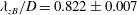 $\unicode[STIX]{x1D706}_{zB}/D=0.822\pm 0.007$
). However, mode A and mode B are not the only two modes to which the wake becomes unstable; a quasi-periodic mode with complex Floquet multipliers is predicted by the stability analysis to occur at
$\unicode[STIX]{x1D706}_{zB}/D=0.822\pm 0.007$
). However, mode A and mode B are not the only two modes to which the wake becomes unstable; a quasi-periodic mode with complex Floquet multipliers is predicted by the stability analysis to occur at
 $Re\simeq 377$
with a critical spanwise wavelength
$Re\simeq 377$
with a critical spanwise wavelength
 $\unicode[STIX]{x1D706}_{zQP}/D\simeq 1.8$
(Blackburn et al.
Reference Blackburn, Marques and Lopez2005).
$\unicode[STIX]{x1D706}_{zQP}/D\simeq 1.8$
(Blackburn et al.
Reference Blackburn, Marques and Lopez2005).
The two-dimensional instantaneous streamwise vorticity contours of modes A and B are presented in figure 9 on top of the line contours of the corresponding base-flow spanwise vorticity. Mode A and mode B are quite different in terms of the spatio-temporal symmetry. Mode A reveals the odd reflection-translation (RT) symmetry
 $\tilde{\unicode[STIX]{x1D714}}_{x}(x,y,z,t)=-\tilde{\unicode[STIX]{x1D714}}_{x}(x,-y,z,t+T/2)$
, for the streamwise vorticity of the Floquet mode swaps signs between each Strouhal vortex pair; mode B exhibits the even RT symmetry
$\tilde{\unicode[STIX]{x1D714}}_{x}(x,y,z,t)=-\tilde{\unicode[STIX]{x1D714}}_{x}(x,-y,z,t+T/2)$
, for the streamwise vorticity of the Floquet mode swaps signs between each Strouhal vortex pair; mode B exhibits the even RT symmetry
 $\tilde{\unicode[STIX]{x1D714}}_{x}(x,y,z,t)=\tilde{\unicode[STIX]{x1D714}}_{x}(x,-y,z,t+T/2)$
, for the streamwise vorticity of the Floquet mode has the same sign on both sides of the wake centreline. It can be observed that mode B decays downstream much more quickly than mode A. It can also be observed that mode A has stronger streamwise vorticity contours in the base flow vortex cores, while for mode B, stronger three-dimensional structures are observed in the shear layers that link the cores (Williamson Reference Williamson1996; Barkley & Henderson Reference Barkley and Henderson1996; Carmo et al.
Reference Carmo, Meneghini and Sherwin2010).
$\tilde{\unicode[STIX]{x1D714}}_{x}(x,y,z,t)=\tilde{\unicode[STIX]{x1D714}}_{x}(x,-y,z,t+T/2)$
, for the streamwise vorticity of the Floquet mode has the same sign on both sides of the wake centreline. It can be observed that mode B decays downstream much more quickly than mode A. It can also be observed that mode A has stronger streamwise vorticity contours in the base flow vortex cores, while for mode B, stronger three-dimensional structures are observed in the shear layers that link the cores (Williamson Reference Williamson1996; Barkley & Henderson Reference Barkley and Henderson1996; Carmo et al.
Reference Carmo, Meneghini and Sherwin2010).

Figure 8. Flow around a bare circular cylinder. (a) Variation of the modulus of the leading Floquet multiplier with the non-dimensional spanwise wavenumber
 $\unicode[STIX]{x1D6FD}D$
, (b) neutral stability curves.
$\unicode[STIX]{x1D6FD}D$
, (b) neutral stability curves.

Figure 9. Two-dimensional streamwise perturbation vorticity contours of a bare circular cylinder. Spanwise vorticity of base flow is overlaid as solid lines. (a) Mode A
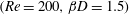 $(Re=200,\unicode[STIX]{x1D6FD}D=1.5)$
; (b) Mode B
$(Re=200,\unicode[STIX]{x1D6FD}D=1.5)$
; (b) Mode B
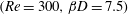 $(Re=300,\unicode[STIX]{x1D6FD}D=7.5)$
.
$(Re=300,\unicode[STIX]{x1D6FD}D=7.5)$
.
3.4.2 Cylinder with dual splitter plates
After summarizing the secondary instability emerging in the wake of flow past a bare cylinder, the effect of the PDSPs on the wake transition was examined, and the results for the secondary instabilities are presented and analysed in detail.
Figure 10 presents the modulus of the Floquet multiplier as a function of the non-dimensional perturbation spanwise wavenumber (left-hand side) and the corresponding neutral stability curves (right-hand side), for four different configurations with
 $L/D=1.0$
and various attachment angles ranging from
$L/D=1.0$
and various attachment angles ranging from
 $\unicode[STIX]{x1D6FC}=20^{\circ }$
to
$\unicode[STIX]{x1D6FC}=20^{\circ }$
to
 $\unicode[STIX]{x1D6FC}=80^{\circ }$
.
$\unicode[STIX]{x1D6FC}=80^{\circ }$
.

Figure 10. Flow around a circular cylinder with attached PDSPs with
 $L/D=1.0$
, for different attachment angles
$L/D=1.0$
, for different attachment angles
 $\unicode[STIX]{x1D6FC}$
: (a,b)
$\unicode[STIX]{x1D6FC}$
: (a,b)
 $20^{\circ }$
; (c,d)
$20^{\circ }$
; (c,d)
 $40^{\circ }$
; (e,f)
$40^{\circ }$
; (e,f)
 $60^{\circ }$
; (g,h)
$60^{\circ }$
; (g,h)
 $80^{\circ }$
. Left-hand images (a,c,e,g), variation of the modulus of the leading Floquet multiplier with the non-dimensional spanwise wavenumber
$80^{\circ }$
. Left-hand images (a,c,e,g), variation of the modulus of the leading Floquet multiplier with the non-dimensional spanwise wavenumber
 $\unicode[STIX]{x1D6FD}D$
; right-hand images (b,d,f,h), neutral stability curves.
$\unicode[STIX]{x1D6FD}D$
; right-hand images (b,d,f,h), neutral stability curves.
Figure 10(a,b) shows the results for the
 $\unicode[STIX]{x1D6FC}=20^{\circ }$
case. It can be seen that the two-dimensional flow is already unstable to infinitesimal three-dimensional perturbations for
$\unicode[STIX]{x1D6FC}=20^{\circ }$
case. It can be seen that the two-dimensional flow is already unstable to infinitesimal three-dimensional perturbations for
 $Re=200$
. Unlike the scenarios for the bare circular cylinder, this three-dimensional mode is not mode A but a mode with positive real multipliers for much smaller spanwise wavenumbers, here named A
$Re=200$
. Unlike the scenarios for the bare circular cylinder, this three-dimensional mode is not mode A but a mode with positive real multipliers for much smaller spanwise wavenumbers, here named A
 $^{\prime }$
, for which the critical Reynolds number is 185. As
$^{\prime }$
, for which the critical Reynolds number is 185. As
 $Re$
increases to 215, mode A appears with a critical spanwise wavelength
$Re$
increases to 215, mode A appears with a critical spanwise wavelength
 $\unicode[STIX]{x1D706}_{zA}/D=5.347$
(
$\unicode[STIX]{x1D706}_{zA}/D=5.347$
(
 $\unicode[STIX]{x1D6FD}_{zA}D=1.175$
), as shown in figure 10(a). As
$\unicode[STIX]{x1D6FD}_{zA}D=1.175$
), as shown in figure 10(a). As
 $Re$
increases further, the flow is unstable to mode B, at a critical Reynolds number of 273 with a spanwise wavelength
$Re$
increases further, the flow is unstable to mode B, at a critical Reynolds number of 273 with a spanwise wavelength
 $\unicode[STIX]{x1D706}_{zB}/D=1.203$
(
$\unicode[STIX]{x1D706}_{zB}/D=1.203$
(
 $\unicode[STIX]{x1D6FD}_{zB}D=5.225$
), and mode QP, at a critical Reynolds number 287 with a spanwise wavelength
$\unicode[STIX]{x1D6FD}_{zB}D=5.225$
), and mode QP, at a critical Reynolds number 287 with a spanwise wavelength
 $\unicode[STIX]{x1D706}_{zQP}/D=2.539$
(
$\unicode[STIX]{x1D706}_{zQP}/D=2.539$
(
 $\unicode[STIX]{x1D6FD}_{zQP}D=2.475$
). From the neutral stability curves displayed in figure 10(b), it can be seen that because of the existence of mode A
$\unicode[STIX]{x1D6FD}_{zQP}D=2.475$
). From the neutral stability curves displayed in figure 10(b), it can be seen that because of the existence of mode A
 $^{\prime }$
, the wakes of this configuration are unstable for arbitrarily small spanwise wavenumber perturbations for
$^{\prime }$
, the wakes of this configuration are unstable for arbitrarily small spanwise wavenumber perturbations for
 $Re\geqslant 185$
. In contrast, the wake of a bare circular cylinder is always stable as
$Re\geqslant 185$
. In contrast, the wake of a bare circular cylinder is always stable as
 $\unicode[STIX]{x1D6FD}D\rightarrow 0$
. This is surprising since the wake transition of the cylinder with PDSPs is very different from that of the bare cylinder. A similar phenomenon is observed in the work of Kevlahan (Reference Kevlahan2007), in which the flow is found to be generally unstable as
$\unicode[STIX]{x1D6FD}D\rightarrow 0$
. This is surprising since the wake transition of the cylinder with PDSPs is very different from that of the bare cylinder. A similar phenomenon is observed in the work of Kevlahan (Reference Kevlahan2007), in which the flow is found to be generally unstable as
 $\unicode[STIX]{x1D706}_{z}/D\rightarrow \infty$
in the wake of both tightly packed rotated and in-line circular cylinder arrays. They attributed this behaviour to the curvature of the function
$\unicode[STIX]{x1D706}_{z}/D\rightarrow \infty$
in the wake of both tightly packed rotated and in-line circular cylinder arrays. They attributed this behaviour to the curvature of the function
 $\left|\unicode[STIX]{x1D707}\right|$
(
$\left|\unicode[STIX]{x1D707}\right|$
(
 $\unicode[STIX]{x1D6FD}D$
) at
$\unicode[STIX]{x1D6FD}D$
) at
 $\unicode[STIX]{x1D6FD}D=0$
. This is also the case for the current investigation, for the second derivative of this function is positive for the
$\unicode[STIX]{x1D6FD}D=0$
. This is also the case for the current investigation, for the second derivative of this function is positive for the
 $\unicode[STIX]{x1D6FC}=20^{\circ }$
case, while it is negative for the bare cylinder case, as shown in figures 10(a) and 8(a), respectively.
$\unicode[STIX]{x1D6FC}=20^{\circ }$
case, while it is negative for the bare cylinder case, as shown in figures 10(a) and 8(a), respectively.
At
 $\unicode[STIX]{x1D6FC}=40^{\circ }$
, as shown in figure 10(c,d), the wake first becomes unstable to a moderate wavelength mode with positive real multipliers at a critical Reynolds number 255 with
$\unicode[STIX]{x1D6FC}=40^{\circ }$
, as shown in figure 10(c,d), the wake first becomes unstable to a moderate wavelength mode with positive real multipliers at a critical Reynolds number 255 with
 $\unicode[STIX]{x1D706}_{zB^{\prime }}/D=2.349$
(
$\unicode[STIX]{x1D706}_{zB^{\prime }}/D=2.349$
(
 $\unicode[STIX]{x1D6FD}_{zB^{\prime }}D=2.675$
). This mode is topologically analogous to mode B
$\unicode[STIX]{x1D6FD}_{zB^{\prime }}D=2.675$
). This mode is topologically analogous to mode B
 $^{\prime }$
of the elongated cylinder wake in the work of Ryan et al. (Reference Ryan, Thompson and Hourigan2005). As
$^{\prime }$
of the elongated cylinder wake in the work of Ryan et al. (Reference Ryan, Thompson and Hourigan2005). As
 $Re$
is increased, the instability mode A
$Re$
is increased, the instability mode A
 $^{\prime }$
emerges with a critical Reynolds number of
$^{\prime }$
emerges with a critical Reynolds number of
 $Re_{A^{\prime }}=270$
and a spanwise wavelength of
$Re_{A^{\prime }}=270$
and a spanwise wavelength of
 $\unicode[STIX]{x1D706}_{zA^{\prime }}/D=17.952$
(
$\unicode[STIX]{x1D706}_{zA^{\prime }}/D=17.952$
(
 $\unicode[STIX]{x1D6FD}_{zA^{\prime }}D=0.35$
), followed by mode A with a critical Reynolds number of
$\unicode[STIX]{x1D6FD}_{zA^{\prime }}D=0.35$
), followed by mode A with a critical Reynolds number of
 $Re_{A}=279$
and a spanwise wavelength of
$Re_{A}=279$
and a spanwise wavelength of
 $\unicode[STIX]{x1D706}_{zA}/D=4.654$
(
$\unicode[STIX]{x1D706}_{zA}/D=4.654$
(
 $\unicode[STIX]{x1D6FD}_{zA}D=1.35$
). Another instability mode, mode B, appears in a higher wavenumber region for a higher
$\unicode[STIX]{x1D6FD}_{zA}D=1.35$
). Another instability mode, mode B, appears in a higher wavenumber region for a higher
 $Re$
. In the stability curves of this configuration, it can be observed that the lower branch of mode A
$Re$
. In the stability curves of this configuration, it can be observed that the lower branch of mode A
 $^{\prime }$
is quite small but not zero. Therefore, the instability wavelength of mode A
$^{\prime }$
is quite small but not zero. Therefore, the instability wavelength of mode A
 $^{\prime }$
is fairly broad for this configuration.
$^{\prime }$
is fairly broad for this configuration.
For the case of
 $\unicode[STIX]{x1D6FC}=60^{\circ }$
, the results in figure 10(e,f) show that the flow is unstable to three topologically different instability modes, which appear in sequence as
$\unicode[STIX]{x1D6FC}=60^{\circ }$
, the results in figure 10(e,f) show that the flow is unstable to three topologically different instability modes, which appear in sequence as
 $Re$
increases. At a Reynolds number of 260, the wake first becomes linearly unstable to the mode A
$Re$
increases. At a Reynolds number of 260, the wake first becomes linearly unstable to the mode A
 $^{\prime }$
instability for a wavelength of
$^{\prime }$
instability for a wavelength of
 $\unicode[STIX]{x1D706}_{zA^{\prime }}/D=31.416$
(
$\unicode[STIX]{x1D706}_{zA^{\prime }}/D=31.416$
(
 $\unicode[STIX]{x1D6FD}_{zA^{\prime }}D=0.2$
). As shown in figure 10(f), the flow is also unstable for arbitrarily small spanwise wavenumber perturbations for
$\unicode[STIX]{x1D6FD}_{zA^{\prime }}D=0.2$
). As shown in figure 10(f), the flow is also unstable for arbitrarily small spanwise wavenumber perturbations for
 $Re\geqslant 275$
due to the presence of the mode A
$Re\geqslant 275$
due to the presence of the mode A
 $^{\prime }$
instability. The other two instability modes are mode B
$^{\prime }$
instability. The other two instability modes are mode B
 $^{\prime }$
and mode A, appearing at
$^{\prime }$
and mode A, appearing at
 $Re_{B^{\prime }}=268$
with
$Re_{B^{\prime }}=268$
with
 $\unicode[STIX]{x1D706}_{zB^{\prime }}/D=2.285$
(
$\unicode[STIX]{x1D706}_{zB^{\prime }}/D=2.285$
(
 $\unicode[STIX]{x1D6FD}_{zB^{\prime }}D=2.75$
) and
$\unicode[STIX]{x1D6FD}_{zB^{\prime }}D=2.75$
) and
 $Re_{A}=305$
with
$Re_{A}=305$
with
 $\unicode[STIX]{x1D706}_{zA}/D=4.707$
(
$\unicode[STIX]{x1D706}_{zA}/D=4.707$
(
 $\unicode[STIX]{x1D6FD}_{zA}D=1.335$
), respectively.
$\unicode[STIX]{x1D6FD}_{zA}D=1.335$
), respectively.
The secondary instability scenario in the flow around the configuration with
 $\unicode[STIX]{x1D6FC}=80^{\circ }$
is more complicated, for the five topologically different modes exhibited in the previous cases were identified, as illustrated in figure 10(g,h). The first instability mode, which emerges at a critical Reynolds number of 207 with
$\unicode[STIX]{x1D6FC}=80^{\circ }$
is more complicated, for the five topologically different modes exhibited in the previous cases were identified, as illustrated in figure 10(g,h). The first instability mode, which emerges at a critical Reynolds number of 207 with
 $\unicode[STIX]{x1D706}_{zA^{\prime }}/D=26.737$
(
$\unicode[STIX]{x1D706}_{zA^{\prime }}/D=26.737$
(
 $\unicode[STIX]{x1D6FD}_{zA^{\prime }}D=0.235$
), is mode A
$\unicode[STIX]{x1D6FD}_{zA^{\prime }}D=0.235$
), is mode A
 $^{\prime }$
. Similar to the case of
$^{\prime }$
. Similar to the case of
 $\unicode[STIX]{x1D6FC}=40^{\circ }$
, the wake of this configuration is also unstable for perturbations with quite small spanwise wavenumbers. The following mode is instability mode A, which appears at
$\unicode[STIX]{x1D6FC}=40^{\circ }$
, the wake of this configuration is also unstable for perturbations with quite small spanwise wavenumbers. The following mode is instability mode A, which appears at
 $Re_{A}=230$
with
$Re_{A}=230$
with
 $\unicode[STIX]{x1D706}_{zA}/D=5.236$
(
$\unicode[STIX]{x1D706}_{zA}/D=5.236$
(
 $\unicode[STIX]{x1D6FD}_{zA}D=1.2$
). The next instability mode, which appears at a critical Reynolds number of 240 with
$\unicode[STIX]{x1D6FD}_{zA}D=1.2$
). The next instability mode, which appears at a critical Reynolds number of 240 with
 $\unicode[STIX]{x1D706}_{zB^{\prime }}/D=2.762$
(
$\unicode[STIX]{x1D706}_{zB^{\prime }}/D=2.762$
(
 $\unicode[STIX]{x1D6FD}_{zB^{\prime }}D=2.275$
), is mode B
$\unicode[STIX]{x1D6FD}_{zB^{\prime }}D=2.275$
), is mode B
 $^{\prime }$
. As shown by the neutral stability curves, the unstable region of this mode is obviously narrowing with increasing
$^{\prime }$
. As shown by the neutral stability curves, the unstable region of this mode is obviously narrowing with increasing
 $Re$
, which means that this mode could probably disappear with a further increase in
$Re$
, which means that this mode could probably disappear with a further increase in
 $Re$
. The critical Reynolds numbers for the last two modes, mode B and mode QP, are 292 with
$Re$
. The critical Reynolds numbers for the last two modes, mode B and mode QP, are 292 with
 $\unicode[STIX]{x1D706}_{zB}/D=0.959$
(
$\unicode[STIX]{x1D706}_{zB}/D=0.959$
(
 $\unicode[STIX]{x1D6FD}_{zB}D=6.55$
) and 330 with
$\unicode[STIX]{x1D6FD}_{zB}D=6.55$
) and 330 with
 $\unicode[STIX]{x1D706}_{zQP}/D=2.06$
(
$\unicode[STIX]{x1D706}_{zQP}/D=2.06$
(
 $\unicode[STIX]{x1D6FD}_{zQP}D=3.05$
), respectively.
$\unicode[STIX]{x1D6FD}_{zQP}D=3.05$
), respectively.
The effects of
 $L/D$
on the secondary instability were also studied. Since the minimum values of the drag and lift coefficients were achieved in the range of
$L/D$
on the secondary instability were also studied. Since the minimum values of the drag and lift coefficients were achieved in the range of
 $50^{\circ }\leqslant \unicode[STIX]{x1D6FC}\leqslant 60^{\circ }$
for
$50^{\circ }\leqslant \unicode[STIX]{x1D6FC}\leqslant 60^{\circ }$
for
 $L/D=1.0$
, the configurations with a constant attachment angle
$L/D=1.0$
, the configurations with a constant attachment angle
 $\unicode[STIX]{x1D6FC}=60^{\circ }$
were selected, with
$\unicode[STIX]{x1D6FC}=60^{\circ }$
were selected, with
 $L/D$
equal to 0.25, 0.5, 0.75 and 1.25, as shown in figure 11.
$L/D$
equal to 0.25, 0.5, 0.75 and 1.25, as shown in figure 11.
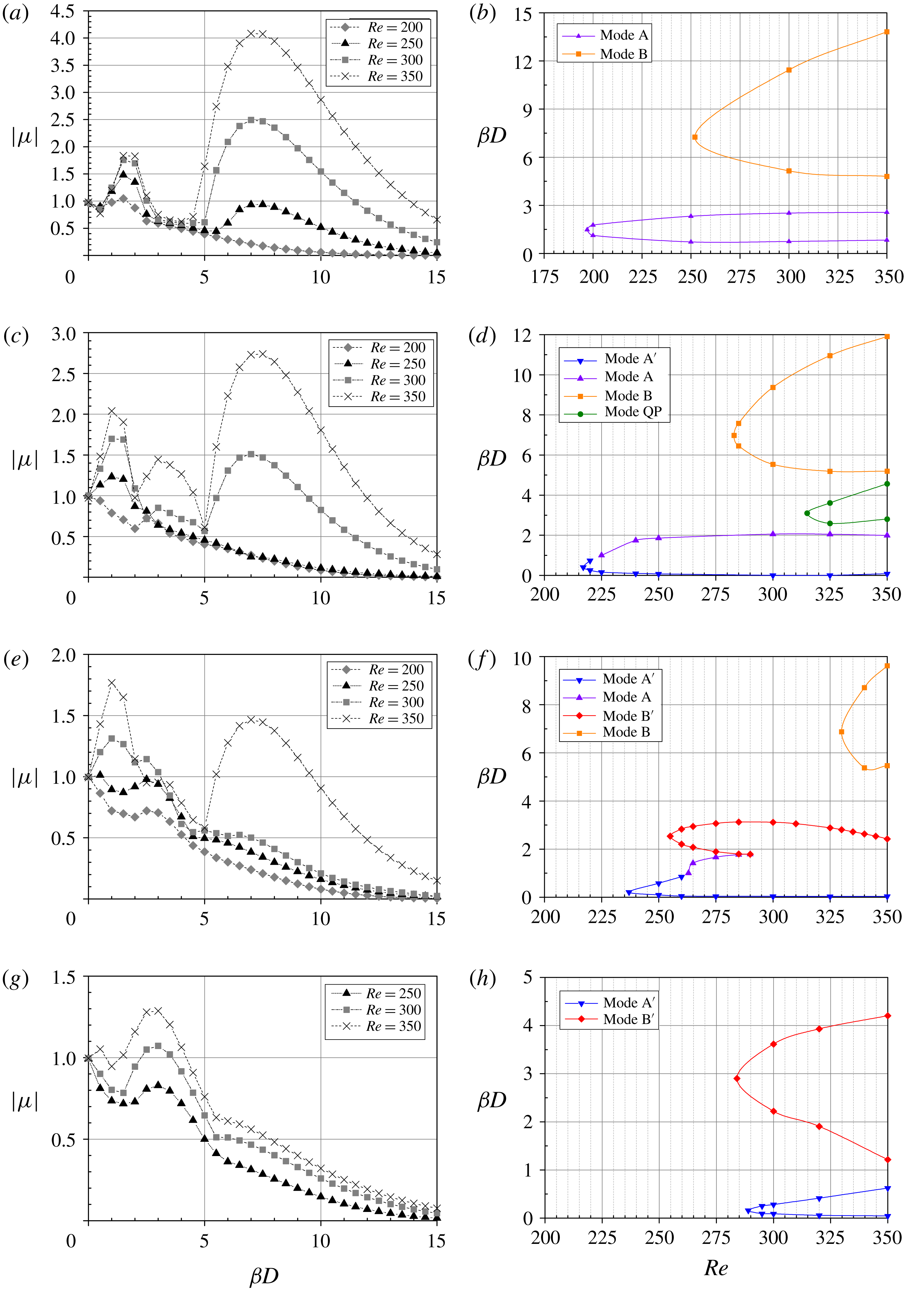
Figure 11. Flow around a circular cylinder with attached PDSPs with
 $\unicode[STIX]{x1D6FC}=60^{\circ }$
, for different splitter plate lengths
$\unicode[STIX]{x1D6FC}=60^{\circ }$
, for different splitter plate lengths
 $L/D$
: (a,b) 0.25; (c,d)
$L/D$
: (a,b) 0.25; (c,d)
 $0.5$
; (e,f)
$0.5$
; (e,f)
 $0.75$
; (g,h)
$0.75$
; (g,h)
 $1.25$
. Left-hand images (a,c,e,g), variation of the modulus of the leading Floquet multiplier with the non-dimensional spanwise wavenumber
$1.25$
. Left-hand images (a,c,e,g), variation of the modulus of the leading Floquet multiplier with the non-dimensional spanwise wavenumber
 $\unicode[STIX]{x1D6FD}D$
; right-hand images (b,d,f,h), neutral stability curves.
$\unicode[STIX]{x1D6FD}D$
; right-hand images (b,d,f,h), neutral stability curves.
For the case of very short splitter plates
 $(L/D=0.25)$
, the results are very similar to those observed in the wake of a bare cylinder, as depicted in figure 11(a,b). The two noticeable peaks with positive real Floquet multipliers in figure 11(a) correspond to mode A (lower
$(L/D=0.25)$
, the results are very similar to those observed in the wake of a bare cylinder, as depicted in figure 11(a,b). The two noticeable peaks with positive real Floquet multipliers in figure 11(a) correspond to mode A (lower
 $\unicode[STIX]{x1D6FD}D$
) and mode B (higher
$\unicode[STIX]{x1D6FD}D$
) and mode B (higher
 $\unicode[STIX]{x1D6FD}D$
). Also, a least unstable mode with complex Floquet multipliers exists for intermediate wavenumbers between the two peaks. The neutral stability curves presented in figure 11(b) show that the critical Reynolds number and the corresponding wavelength for mode A are 197 and
$\unicode[STIX]{x1D6FD}D$
). Also, a least unstable mode with complex Floquet multipliers exists for intermediate wavenumbers between the two peaks. The neutral stability curves presented in figure 11(b) show that the critical Reynolds number and the corresponding wavelength for mode A are 197 and
 $4.26$
(
$4.26$
(
 $\unicode[STIX]{x1D6FD}_{zA}D=1.475$
), respectively, both of which are slightly higher than their counterparts in the bare cylinder case. Meanwhile, the onset of mode B occurs slightly earlier in terms of the Reynolds numbers (
$\unicode[STIX]{x1D6FD}_{zA}D=1.475$
), respectively, both of which are slightly higher than their counterparts in the bare cylinder case. Meanwhile, the onset of mode B occurs slightly earlier in terms of the Reynolds numbers (
 $Re_{B}=252$
) than in the bare cylinder case. The critical spanwise wavelength of this instability mode is
$Re_{B}=252$
) than in the bare cylinder case. The critical spanwise wavelength of this instability mode is
 $\unicode[STIX]{x1D706}_{zB}/D=0.867$
(
$\unicode[STIX]{x1D706}_{zB}/D=0.867$
(
 $\unicode[STIX]{x1D6FD}_{zB}D=7.25$
), which is larger than that of mode B for the bare cylinder case.
$\unicode[STIX]{x1D6FD}_{zB}D=7.25$
), which is larger than that of mode B for the bare cylinder case.
If the length of the splitter plates is increased to
 $L/D=0.5$
, the secondary instability scenario would change. In fact, as shown in figure 11(c,d), compared with the bare cylinder case, one more transition mode, mode A
$L/D=0.5$
, the secondary instability scenario would change. In fact, as shown in figure 11(c,d), compared with the bare cylinder case, one more transition mode, mode A
 $^{\prime }$
, is observed, to which the wake of this configuration is first to become unstable. The instability mode emerges at its bifurcation point of
$^{\prime }$
, is observed, to which the wake of this configuration is first to become unstable. The instability mode emerges at its bifurcation point of
 $Re_{A^{\prime }}=217$
, with a spanwise wavelength of
$Re_{A^{\prime }}=217$
, with a spanwise wavelength of
 $\unicode[STIX]{x1D706}_{zA^{\prime }}/D=14.784$
(
$\unicode[STIX]{x1D706}_{zA^{\prime }}/D=14.784$
(
 $\unicode[STIX]{x1D6FD}_{zA^{\prime }}D=0.425$
). The critical Reynolds number for mode A is 225, which is quite close to that for mode A
$\unicode[STIX]{x1D6FD}_{zA^{\prime }}D=0.425$
). The critical Reynolds number for mode A is 225, which is quite close to that for mode A
 $^{\prime }$
, and the unstable eigenmode has a spanwise wavelength of
$^{\prime }$
, and the unstable eigenmode has a spanwise wavelength of
 $\unicode[STIX]{x1D706}_{zA}/D=5.03$
(
$\unicode[STIX]{x1D706}_{zA}/D=5.03$
(
 $\unicode[STIX]{x1D6FD}_{zA}D=1.25$
). The appearance of mode B is also delayed in terms of
$\unicode[STIX]{x1D6FD}_{zA}D=1.25$
). The appearance of mode B is also delayed in terms of
 $Re$
, at
$Re$
, at
 $Re_{B}=283$
, with a larger critical spanwise wavelength of
$Re_{B}=283$
, with a larger critical spanwise wavelength of
 $\unicode[STIX]{x1D706}_{zB}/D=0.901$
(
$\unicode[STIX]{x1D706}_{zB}/D=0.901$
(
 $\unicode[STIX]{x1D6FD}_{zB}D=6.975$
). Moreover, the quasi-periodic mode with complex Floquet multipliers for intermediate wavenumbers is detected at
$\unicode[STIX]{x1D6FD}_{zB}D=6.975$
). Moreover, the quasi-periodic mode with complex Floquet multipliers for intermediate wavenumbers is detected at
 $Re_{QP}=315$
with a wavelength of
$Re_{QP}=315$
with a wavelength of
 $\unicode[STIX]{x1D706}_{zQP}/D=2.027$
(
$\unicode[STIX]{x1D706}_{zQP}/D=2.027$
(
 $\unicode[STIX]{x1D6FD}_{zQP}D=3.1$
). This mode appears considerably earlier compared with that in the bare cylinder case.
$\unicode[STIX]{x1D6FD}_{zQP}D=3.1$
). This mode appears considerably earlier compared with that in the bare cylinder case.
The results of the case of
 $L/D=0.75$
are shown in figure 11(e,f). Compared with the case of
$L/D=0.75$
are shown in figure 11(e,f). Compared with the case of
 $L/D=0.5$
, the appearances of modes A
$L/D=0.5$
, the appearances of modes A
 $^{\prime }$
, A and B are further delayed in terms of
$^{\prime }$
, A and B are further delayed in terms of
 $Re$
. The critical Reynolds numbers for the three modes are 237, 263 and 330, with corresponding spanwise wavelengths of
$Re$
. The critical Reynolds numbers for the three modes are 237, 263 and 330, with corresponding spanwise wavelengths of
 $\unicode[STIX]{x1D706}_{zA^{\prime }}/D=25.133$
(
$\unicode[STIX]{x1D706}_{zA^{\prime }}/D=25.133$
(
 $\unicode[STIX]{x1D6FD}_{zA^{\prime }}D=0.25$
),
$\unicode[STIX]{x1D6FD}_{zA^{\prime }}D=0.25$
),
 $\unicode[STIX]{x1D706}_{zA}/D=5.464$
(
$\unicode[STIX]{x1D706}_{zA}/D=5.464$
(
 $\unicode[STIX]{x1D6FD}_{zA}D=1.15$
) and
$\unicode[STIX]{x1D6FD}_{zA}D=1.15$
) and
 $\unicode[STIX]{x1D706}_{zB}/D=0.914$
(
$\unicode[STIX]{x1D706}_{zB}/D=0.914$
(
 $\unicode[STIX]{x1D6FD}_{zB}D=6.875$
), respectively. From the neutral stability curves, mode A
$\unicode[STIX]{x1D6FD}_{zB}D=6.875$
), respectively. From the neutral stability curves, mode A
 $^{\prime }$
is observed to develop in the wake for arbitrarily small spanwise wavenumber perturbations for
$^{\prime }$
is observed to develop in the wake for arbitrarily small spanwise wavenumber perturbations for
 $Re>250$
. In this case, the intermediate wavelength mode is no longer mode QP but mode B
$Re>250$
. In this case, the intermediate wavelength mode is no longer mode QP but mode B
 $^{\prime }$
, which appears at its bifurcation point of
$^{\prime }$
, which appears at its bifurcation point of
 $Re=255$
, with a spanwise wavelength of
$Re=255$
, with a spanwise wavelength of
 $\unicode[STIX]{x1D706}_{zB^{\prime }}/D=2.479$
(
$\unicode[STIX]{x1D706}_{zB^{\prime }}/D=2.479$
(
 $\unicode[STIX]{x1D6FD}_{zB^{\prime }}D=2.535$
).
$\unicode[STIX]{x1D6FD}_{zB^{\prime }}D=2.535$
).
For
 $L/D=1.25$
, the transition modes observed in the bare cylinder case completely disappear and two topologically different modes emerge, as displayed in figure 11(g,h). The critical Reynolds numbers for the two modes, mode A
$L/D=1.25$
, the transition modes observed in the bare cylinder case completely disappear and two topologically different modes emerge, as displayed in figure 11(g,h). The critical Reynolds numbers for the two modes, mode A
 $^{\prime }$
and mode B
$^{\prime }$
and mode B
 $^{\prime }$
, are quite close. The onset of mode A
$^{\prime }$
, are quite close. The onset of mode A
 $^{\prime }$
is predicted to occur at
$^{\prime }$
is predicted to occur at
 $Re_{A^{\prime }}=289$
, with a spanwise wavelength of
$Re_{A^{\prime }}=289$
, with a spanwise wavelength of
 $\unicode[STIX]{x1D706}_{zA^{\prime }}/D=39.27$
(
$\unicode[STIX]{x1D706}_{zA^{\prime }}/D=39.27$
(
 $\unicode[STIX]{x1D6FD}_{zA^{\prime }}D=0.16$
), and that of mode B
$\unicode[STIX]{x1D6FD}_{zA^{\prime }}D=0.16$
), and that of mode B
 $^{\prime }$
is slightly earlier, at
$^{\prime }$
is slightly earlier, at
 $Re_{B^{\prime }}=284$
with a spanwise wavelength of
$Re_{B^{\prime }}=284$
with a spanwise wavelength of
 $\unicode[STIX]{x1D706}_{zB^{\prime }}/D=2.167$
(
$\unicode[STIX]{x1D706}_{zB^{\prime }}/D=2.167$
(
 $\unicode[STIX]{x1D6FD}_{zB^{\prime }}D=2.9$
). Again, the flow is unstable to mode A
$\unicode[STIX]{x1D6FD}_{zB^{\prime }}D=2.9$
). Again, the flow is unstable to mode A
 $^{\prime }$
for quite small spanwise perturbation wavenumbers.
$^{\prime }$
for quite small spanwise perturbation wavenumbers.
3.4.3 Mode characteristics
In order to reveal the characteristics of the modes found in the above section, images of the two-dimensional topology for each mode are presented for the specific case of
 $\unicode[STIX]{x1D6FC}=40^{\circ }$
and
$\unicode[STIX]{x1D6FC}=40^{\circ }$
and
 $L/D=1.0$
. The mode topology adopted here is representative of that found for other configurations. These images show the colour contours of the streamwise perturbation vorticity, overlaid with black contour lines denoting the positions of the base-flow vortex cores.
$L/D=1.0$
. The mode topology adopted here is representative of that found for other configurations. These images show the colour contours of the streamwise perturbation vorticity, overlaid with black contour lines denoting the positions of the base-flow vortex cores.
Figure 12(a,c) presents a comparison of structures between mode A and mode A
 $^{\prime }$
at
$^{\prime }$
at
 $Re=300$
. It is evident that the instability mode A depicted in figure 12(a) shows the same overall near- and far-wake structures and spatio-temporal symmetry as those found in the wake of a bare circular cylinder (shown in figure 9
a). As shown in figure 12(c), mode A
$Re=300$
. It is evident that the instability mode A depicted in figure 12(a) shows the same overall near- and far-wake structures and spatio-temporal symmetry as those found in the wake of a bare circular cylinder (shown in figure 9
a). As shown in figure 12(c), mode A
 $^{\prime }$
has the same spatio-temporal symmetry as mode A, and the near-wake perturbation field distribution of mode A
$^{\prime }$
has the same spatio-temporal symmetry as mode A, and the near-wake perturbation field distribution of mode A
 $^{\prime }$
is quite similar to that of mode A. Specifically, the structures of mode A and mode A
$^{\prime }$
is quite similar to that of mode A. Specifically, the structures of mode A and mode A
 $^{\prime }$
are almost the same in the first two vortices at the rear of the splitter plates. However, substantial distinctions emerge from the third vortex and further downstream. For example, mode A has one blue lobe in the lower portion of the third vortex and one red lobe in the upper portion of this vortex, whereas mode A
$^{\prime }$
are almost the same in the first two vortices at the rear of the splitter plates. However, substantial distinctions emerge from the third vortex and further downstream. For example, mode A has one blue lobe in the lower portion of the third vortex and one red lobe in the upper portion of this vortex, whereas mode A
 $^{\prime }$
has only one blue lobe extending over the entire vortex. This is circled with solid lines in figure 12(a,c). Another example of difference exists in the spatial structures of the braid shear layer, which is indicated by the arrows overlaid on the figure. In this region, the sign of the perturbation vorticity changes once for mode A
$^{\prime }$
has only one blue lobe extending over the entire vortex. This is circled with solid lines in figure 12(a,c). Another example of difference exists in the spatial structures of the braid shear layer, which is indicated by the arrows overlaid on the figure. In this region, the sign of the perturbation vorticity changes once for mode A
 $^{\prime }$
(blue–red), while the sign keeps constant for mode A. It is worth noting that the streamwise perturbation vorticity of mode A
$^{\prime }$
(blue–red), while the sign keeps constant for mode A. It is worth noting that the streamwise perturbation vorticity of mode A
 $^{\prime }$
decays downstream more quickly than that of mode A for the first several shedding cycles. Nevertheless, the perturbation field further downstream shows a higher and more persistent perturbation amplitude in the streamwise perturbation vortex cores of mode A
$^{\prime }$
decays downstream more quickly than that of mode A for the first several shedding cycles. Nevertheless, the perturbation field further downstream shows a higher and more persistent perturbation amplitude in the streamwise perturbation vortex cores of mode A
 $^{\prime }$
, which is not shown in figure 12(c) but can be observed in its three-dimensional reconstruction (figure 13
b) or the three-dimensional direct numerical simulation results (figures 22
c and 23
f).
$^{\prime }$
, which is not shown in figure 12(c) but can be observed in its three-dimensional reconstruction (figure 13
b) or the three-dimensional direct numerical simulation results (figures 22
c and 23
f).

Figure 12. Two-dimensional streamwise perturbation vorticity contours of the circular cylinder with attached PDSPs for
 $\unicode[STIX]{x1D6FC}=40^{\circ }$
and
$\unicode[STIX]{x1D6FC}=40^{\circ }$
and
 $L/D=1.0$
. Spanwise vorticity of base flow is overlaid as solid lines. (a) Mode A (
$L/D=1.0$
. Spanwise vorticity of base flow is overlaid as solid lines. (a) Mode A (
 $Re=300$
,
$Re=300$
,
 $\unicode[STIX]{x1D6FD}D=1.57$
); (b) mode B (
$\unicode[STIX]{x1D6FD}D=1.57$
); (b) mode B (
 $Re=350$
,
$Re=350$
,
 $\unicode[STIX]{x1D6FD}D=6.28$
); (c) mode A
$\unicode[STIX]{x1D6FD}D=6.28$
); (c) mode A
 $^{\prime }$
(
$^{\prime }$
(
 $Re=300$
,
$Re=300$
,
 $\unicode[STIX]{x1D6FD}D=0.52$
); (d) mode B
$\unicode[STIX]{x1D6FD}D=0.52$
); (d) mode B
 $^{\prime }$
(
$^{\prime }$
(
 $Re=350$
,
$Re=350$
,
 $\unicode[STIX]{x1D6FD}D=2.62$
).
$\unicode[STIX]{x1D6FD}D=2.62$
).
An instability mode found by Leontini et al. (Reference Leontini, Lo Jacono and Thompson2015) in the wake of elliptic cylinders, named mode Â, has many features in common with mode A
 $^{\prime }$
, such as the spatio-temporal symmetries and near-wake perturbation field distributions. The critical wavelength of mode  is also very long, for example, approaching
$^{\prime }$
, such as the spatio-temporal symmetries and near-wake perturbation field distributions. The critical wavelength of mode  is also very long, for example, approaching
 $28D$
in the case with
$28D$
in the case with
 $\unicode[STIX]{x1D6E4}=2.4$
(
$\unicode[STIX]{x1D6E4}=2.4$
(
 $\unicode[STIX]{x1D6E4}=$
major/minor axis ratio). In view of these facts, it is reasonable to speculate that the physical mechanism leading to mode A
$\unicode[STIX]{x1D6E4}=$
major/minor axis ratio). In view of these facts, it is reasonable to speculate that the physical mechanism leading to mode A
 $^{\prime }$
is similar to that causing mode  in the wake of elliptic cylinders.
$^{\prime }$
is similar to that causing mode  in the wake of elliptic cylinders.

Figure 13. Three-dimensional view of the unstable Floquet modes combined with the base flow for the configuration with
 $\unicode[STIX]{x1D6FC}=40^{\circ }$
and
$\unicode[STIX]{x1D6FC}=40^{\circ }$
and
 $L/D=1.0$
. (a) Mode A (
$L/D=1.0$
. (a) Mode A (
 $Re=300$
,
$Re=300$
,
 $\unicode[STIX]{x1D6FD}D=1.57$
); (b) mode A
$\unicode[STIX]{x1D6FD}D=1.57$
); (b) mode A
 $^{\prime }$
(
$^{\prime }$
(
 $Re=300$
,
$Re=300$
,
 $\unicode[STIX]{x1D6FD}D=0.52$
); (c) mode B (
$\unicode[STIX]{x1D6FD}D=0.52$
); (c) mode B (
 $Re=350$
,
$Re=350$
,
 $\unicode[STIX]{x1D6FD}D=6.28$
); (d) mode B
$\unicode[STIX]{x1D6FD}D=6.28$
); (d) mode B
 $^{\prime }$
(
$^{\prime }$
(
 $Re=350$
,
$Re=350$
,
 $\unicode[STIX]{x1D6FD}D=2.62$
). Translucent surfaces represent iso-surfaces of
$\unicode[STIX]{x1D6FD}D=2.62$
). Translucent surfaces represent iso-surfaces of
 $|\unicode[STIX]{x1D714}_{z}|$
. Solid red and blue surfaces are iso-surfaces of positive and negative
$|\unicode[STIX]{x1D714}_{z}|$
. Solid red and blue surfaces are iso-surfaces of positive and negative
 $\unicode[STIX]{x1D714}_{x}$
, respectively.
$\unicode[STIX]{x1D714}_{x}$
, respectively.
The spatial structures of the streamwise perturbation vorticity of mode B and mode B
 $^{\prime }$
at
$^{\prime }$
at
 $Re=350$
are illustrated in figure 12(b,d). Mode B depicted in figure 12(b) clearly shows similarities with the corresponding mode in a bare cylinder wake, such as the spatio-temporal symmetry. The main difference exists in the near-wake structure, which could be ascribed to the presence of the splitter plates. Additionally, for the geometry under investigation, the perturbation vorticity of mode B decays slower than that for the bare cylinder.
$Re=350$
are illustrated in figure 12(b,d). Mode B depicted in figure 12(b) clearly shows similarities with the corresponding mode in a bare cylinder wake, such as the spatio-temporal symmetry. The main difference exists in the near-wake structure, which could be ascribed to the presence of the splitter plates. Additionally, for the geometry under investigation, the perturbation vorticity of mode B decays slower than that for the bare cylinder.
For mode B
 $^{\prime }$
, as shown in figure 12(d), the sign of the streamwise vorticity is maintained from one half-cycle to the next, which indicates the same symmetry as mode B. The near-wake structure of mode B
$^{\prime }$
, as shown in figure 12(d), the sign of the streamwise vorticity is maintained from one half-cycle to the next, which indicates the same symmetry as mode B. The near-wake structure of mode B
 $^{\prime }$
is almost the same as that of mode B. However, mode B
$^{\prime }$
is almost the same as that of mode B. However, mode B
 $^{\prime }$
has a distinct structure from the third vortex and further downstream. An example of these distinctions is found by focusing on the vortex that is just shed into the wake and circled with solid lines in figure 12(b,d). The blue lobe in this vortex pervades the braid and vortex core for mode B
$^{\prime }$
has a distinct structure from the third vortex and further downstream. An example of these distinctions is found by focusing on the vortex that is just shed into the wake and circled with solid lines in figure 12(b,d). The blue lobe in this vortex pervades the braid and vortex core for mode B
 $^{\prime }$
, whereas the blue lobe is mainly concentrated in the vortex core for mode B.
$^{\prime }$
, whereas the blue lobe is mainly concentrated in the vortex core for mode B.
As previously mentioned, the instability mode B
 $^{\prime }$
was also identified by Ryan et al. (Reference Ryan, Thompson and Hourigan2005) in stability calculations of the flow around elongated elliptic leading-edge cylinders with
$^{\prime }$
was also identified by Ryan et al. (Reference Ryan, Thompson and Hourigan2005) in stability calculations of the flow around elongated elliptic leading-edge cylinders with
 $AR\geqslant 7.5$
. Striking similarities between the two-dimensional structure of mode B
$AR\geqslant 7.5$
. Striking similarities between the two-dimensional structure of mode B
 $^{\prime }$
are found when comparing figure 12(d) to the results presented in Ryan et al. (Reference Ryan, Thompson and Hourigan2005). The non-dimensional spanwise wavelength of mode B
$^{\prime }$
are found when comparing figure 12(d) to the results presented in Ryan et al. (Reference Ryan, Thompson and Hourigan2005). The non-dimensional spanwise wavelength of mode B
 $^{\prime }$
found in the present investigation is also reasonably close to the value of 2.2 reported in Ryan et al. (Reference Ryan, Thompson and Hourigan2005). The main difference that can be observed is that the braid shear layers of mode B
$^{\prime }$
found in the present investigation is also reasonably close to the value of 2.2 reported in Ryan et al. (Reference Ryan, Thompson and Hourigan2005). The main difference that can be observed is that the braid shear layers of mode B
 $^{\prime }$
in Ryan et al. (Reference Ryan, Thompson and Hourigan2005) decay more slowly, which probably results from the fact that these layers are more elongated due to the much longer geometry.
$^{\prime }$
in Ryan et al. (Reference Ryan, Thompson and Hourigan2005) decay more slowly, which probably results from the fact that these layers are more elongated due to the much longer geometry.
As is well known, the instability leading to mode B is concentrated in the braid shear layer. Nevertheless, this is not true for mode B
 $^{\prime }$
. In figure 12(d), the instability responsible for mode B
$^{\prime }$
. In figure 12(d), the instability responsible for mode B
 $^{\prime }$
is observed to be mainly focused in the wake vortex cores and persist far downstream. This feature of mode B
$^{\prime }$
is observed to be mainly focused in the wake vortex cores and persist far downstream. This feature of mode B
 $^{\prime }$
is much like that of mode A, which means that the elliptic instability may also be involved in the development of mode B
$^{\prime }$
is much like that of mode A, which means that the elliptic instability may also be involved in the development of mode B
 $^{\prime }$
, as Ryan et al. (Reference Ryan, Thompson and Hourigan2005) proposed. Leontini et al. (Reference Leontini, Lo Jacono and Thompson2015) also observed a mode named mode B̂ with a complicated perturbation field distribution similar to that of mode B
$^{\prime }$
, as Ryan et al. (Reference Ryan, Thompson and Hourigan2005) proposed. Leontini et al. (Reference Leontini, Lo Jacono and Thompson2015) also observed a mode named mode B̂ with a complicated perturbation field distribution similar to that of mode B
 $^{\prime }$
, and they speculated that a number of cooperative mechanisms contribute to its growth.
$^{\prime }$
, and they speculated that a number of cooperative mechanisms contribute to its growth.
Corresponding to their two-dimensional topology, the three-dimensional structures of the unstable modes described above are presented in figure 13. For each mode, the three-dimensional topology is obtained by a linear combination of the base flow and a Floquet mode of arbitrary intensity. For uniformity in the visualizations and easy comparison, the spanwise domain for the four modes has been extended out to
 $12D$
.
$12D$
.
The two- and three-dimensional structures of the quasi-periodic modes obtained in the present study will not be presented here, as the determination of these structures from the Floquet modes is not straightforward and is dependent on the phase, as discussed in Blackburn et al. (Reference Blackburn, Marques and Lopez2005).
3.4.4 Mode relationships
From the Floquet multipliers presented in the previous sections, it is not easy to distinguish mode A and mode A
 $^{\prime }$
. For the configurations investigated in the present work, two different relationships between the two modes are found through additional calculations, and two examples are shown in figure 14(a,b). In figure 14(a), two distinct stability branches are observed, and the identification of mode A and mode A
$^{\prime }$
. For the configurations investigated in the present work, two different relationships between the two modes are found through additional calculations, and two examples are shown in figure 14(a,b). In figure 14(a), two distinct stability branches are observed, and the identification of mode A and mode A
 $^{\prime }$
is quite easy. On the other hand, it is difficult to distinguish the two modes from figure 14(b), for the distinction between the branches of mode A and mode A
$^{\prime }$
is quite easy. On the other hand, it is difficult to distinguish the two modes from figure 14(b), for the distinction between the branches of mode A and mode A
 $^{\prime }$
disappears and mode A appears as a continuation of mode A
$^{\prime }$
disappears and mode A appears as a continuation of mode A
 $^{\prime }$
. In cases like this, mode A
$^{\prime }$
. In cases like this, mode A
 $^{\prime }$
gradually changes to mode A with increasing wavenumber, and the only way to distinguish the two modes is to examine the perturbation field distributions.
$^{\prime }$
gradually changes to mode A with increasing wavenumber, and the only way to distinguish the two modes is to examine the perturbation field distributions.
Figure 14(c–k) shows the streamwise perturbation vorticity contours for different spanwise wavenumbers, corresponding to the results of
 $Re=240$
in figure 14(b). The distinction can be made by focusing on the local perturbation structure in the third vortex, as described previously. It can be observed that the contours appear to be constant for spanwise wavenumbers beyond
$Re=240$
in figure 14(b). The distinction can be made by focusing on the local perturbation structure in the third vortex, as described previously. It can be observed that the contours appear to be constant for spanwise wavenumbers beyond
 $\unicode[STIX]{x1D6FD}D=1.2$
. This gradual change is also observed for the configurations with splitter plate lengths of
$\unicode[STIX]{x1D6FD}D=1.2$
. This gradual change is also observed for the configurations with splitter plate lengths of
 $L/D=0.5$
and 0.75, which can be seen from their neutral stability curves (figures 11(d) and 11(f), respectively).
$L/D=0.5$
and 0.75, which can be seen from their neutral stability curves (figures 11(d) and 11(f), respectively).

Figure 14. Variation of the modulus of the leading Floquet multiplier with the spanwise wavenumber
 $\unicode[STIX]{x1D6FD}D$
at (a)
$\unicode[STIX]{x1D6FD}D$
at (a)
 $\unicode[STIX]{x1D6FC}=40^{\circ }$
and (b)
$\unicode[STIX]{x1D6FC}=40^{\circ }$
and (b)
 $\unicode[STIX]{x1D6FC}=80^{\circ }$
. (c–k) Contours of the streamwise perturbation vorticity at the same instant of vortex shedding at
$\unicode[STIX]{x1D6FC}=80^{\circ }$
. (c–k) Contours of the streamwise perturbation vorticity at the same instant of vortex shedding at
 $Re=240$
for spanwise wavenumbers
$Re=240$
for spanwise wavenumbers
 $\unicode[STIX]{x1D6FD}D$
of (c)
$\unicode[STIX]{x1D6FD}D$
of (c)
 $0.7$
, (d)
$0.7$
, (d)
 $0.8$
, (e)
$0.8$
, (e)
 $0.9$
, (f)
$0.9$
, (f)
 $1.0$
, (g)
$1.0$
, (g)
 $1.1$
, (h)
$1.1$
, (h)
 $1.2$
, (i)
$1.2$
, (i)
 $1.3$
, (j)
$1.3$
, (j)
 $1.4$
, (k)
$1.4$
, (k)
 $1.5$
.
$1.5$
.
Similar to mode A and mode A
 $^{\prime }$
, there also exist two different relationships between mode B and mode B
$^{\prime }$
, there also exist two different relationships between mode B and mode B
 $^{\prime }$
. For example, the two modes correspond to two independent branches in figures 10(h) and 11(f), which facilitates their identifications. However, for the case of
$^{\prime }$
. For example, the two modes correspond to two independent branches in figures 10(h) and 11(f), which facilitates their identifications. However, for the case of
 $\unicode[STIX]{x1D6FC}=40^{\circ }$
and
$\unicode[STIX]{x1D6FC}=40^{\circ }$
and
 $L/D=1.0$
, a gradual change from mode B
$L/D=1.0$
, a gradual change from mode B
 $^{\prime }$
to mode B is observed in figures 10(d) and 15(a), which makes the differentiation quite difficult. Thus, the variation in the perturbation field distributions with increasing wavenumber is examined, as shown in figure 15(b–j). It can be observed that the blue lobe in the third vortex that is just shed into the wake shrinks with increasing wavenumber until the wavenumber reaches 5.0. For
$^{\prime }$
to mode B is observed in figures 10(d) and 15(a), which makes the differentiation quite difficult. Thus, the variation in the perturbation field distributions with increasing wavenumber is examined, as shown in figure 15(b–j). It can be observed that the blue lobe in the third vortex that is just shed into the wake shrinks with increasing wavenumber until the wavenumber reaches 5.0. For
 $\unicode[STIX]{x1D6FD}D\geqslant 5.1$
, this blue lobe keeps almost constant and is concentrated in the vortex core, consistent with the previous description of mode B.
$\unicode[STIX]{x1D6FD}D\geqslant 5.1$
, this blue lobe keeps almost constant and is concentrated in the vortex core, consistent with the previous description of mode B.
Gradual changes from one instability mode to another are not uncommon, as a previous stability analysis of the wake behind an inclined flat plate with an attack angle of
 $30^{\circ }$
shows that a quasi-periodic mode appears as the continuation of mode C, shown in figure 5 of Yang et al. (Reference Yang, Pettersen, Andersson and Narasimhamurthy2013). Additionally, in the wake of an inclined elliptical cylinder with
$30^{\circ }$
shows that a quasi-periodic mode appears as the continuation of mode C, shown in figure 5 of Yang et al. (Reference Yang, Pettersen, Andersson and Narasimhamurthy2013). Additionally, in the wake of an inclined elliptical cylinder with
 $\unicode[STIX]{x1D6E4}=2.5$
and an incidence angle of
$\unicode[STIX]{x1D6E4}=2.5$
and an incidence angle of
 $12^{\circ }$
, mode  is observed to gradually change to mode A with increasing wavelength (see figure 16 of Rao et al. (Reference Rao, Leontini, Thompson and Hourigan2017)).
$12^{\circ }$
, mode  is observed to gradually change to mode A with increasing wavelength (see figure 16 of Rao et al. (Reference Rao, Leontini, Thompson and Hourigan2017)).

Figure 15. Variation of the modulus of the leading Floquet multiplier with the spanwise wavenumber
 $\unicode[STIX]{x1D6FD}D$
at (a)
$\unicode[STIX]{x1D6FD}D$
at (a)
 $40^{\circ }$
. (b–j) Contours of the streamwise perturbation vorticity at the same instant of vortex shedding at of
$40^{\circ }$
. (b–j) Contours of the streamwise perturbation vorticity at the same instant of vortex shedding at of
 $Re=330$
for spanwise wavenumbers
$Re=330$
for spanwise wavenumbers
 $\unicode[STIX]{x1D6FD}D$
of (b) 3.0, (c) 3.5, (d) 4.0, (e) 4.5, (f) 4.9, (g) 5.0, (h) 5.1, (i) 5.5, (j) 6.0.
$\unicode[STIX]{x1D6FD}D$
of (b) 3.0, (c) 3.5, (d) 4.0, (e) 4.5, (f) 4.9, (g) 5.0, (h) 5.1, (i) 5.5, (j) 6.0.
3.4.5 Criticalities of instability modes
In order to present a more complete picture of the onsets of the three-dimensional wake instabilities in the presence of PDSPs, the critical Reynolds numbers (
 $Re_{c2}$
) and respective spanwise perturbation wavelengths (
$Re_{c2}$
) and respective spanwise perturbation wavelengths (
 $\unicode[STIX]{x1D706}_{cr}$
) varying according to the cylinder–plate configurations are plotted in figure 16.
$\unicode[STIX]{x1D706}_{cr}$
) varying according to the cylinder–plate configurations are plotted in figure 16.

Figure 16. Variation of the critical Reynolds number and respective spanwise perturbation wavelength with the attachment angle
 $\unicode[STIX]{x1D6FC}$
(a–c) and the splitter plate length
$\unicode[STIX]{x1D6FC}$
(a–c) and the splitter plate length
 $L/D$
(d–f).
$L/D$
(d–f).
Figure 16(a) shows the critical Reynolds number of each instability mode as a function of
 $\unicode[STIX]{x1D6FC}$
; the corresponding critical wavelengths are presented in figure 16(b,c). As shown,
$\unicode[STIX]{x1D6FC}$
; the corresponding critical wavelengths are presented in figure 16(b,c). As shown,
 $Re_{c2}$
for each of the synchronous modes first increases and then decreases with
$Re_{c2}$
for each of the synchronous modes first increases and then decreases with
 $\unicode[STIX]{x1D6FC}$
; modes A, B and B
$\unicode[STIX]{x1D6FC}$
; modes A, B and B
 $^{\prime }$
hit their peaks at
$^{\prime }$
hit their peaks at
 $\unicode[STIX]{x1D6FC}=60^{\circ }$
, and mode A
$\unicode[STIX]{x1D6FC}=60^{\circ }$
, and mode A
 $^{\prime }$
hits its peak at
$^{\prime }$
hits its peak at
 $\unicode[STIX]{x1D6FC}=40^{\circ }$
. This trend for mode B
$\unicode[STIX]{x1D6FC}=40^{\circ }$
. This trend for mode B
 $^{\prime }$
is weak in comparison, and its
$^{\prime }$
is weak in comparison, and its
 $Re_{c2}$
has relatively small fluctuations. The quasi-periodic mode disappears between
$Re_{c2}$
has relatively small fluctuations. The quasi-periodic mode disappears between
 $\unicode[STIX]{x1D6FC}=20^{\circ }$
and
$\unicode[STIX]{x1D6FC}=20^{\circ }$
and
 $\unicode[STIX]{x1D6FC}=80^{\circ }$
. The critical wavelengths are found to have a complicated relationship with
$\unicode[STIX]{x1D6FC}=80^{\circ }$
. The critical wavelengths are found to have a complicated relationship with
 $\unicode[STIX]{x1D6FC}$
.
$\unicode[STIX]{x1D6FC}$
.
 $\unicode[STIX]{x1D706}_{cr}$
for both modes A and B
$\unicode[STIX]{x1D706}_{cr}$
for both modes A and B
 $^{\prime }$
first decreases and then increases. For mode B,
$^{\prime }$
first decreases and then increases. For mode B,
 $\unicode[STIX]{x1D706}_{cr}$
first mildly increases until
$\unicode[STIX]{x1D706}_{cr}$
first mildly increases until
 $\unicode[STIX]{x1D6FC}=40^{\circ }$
and then gradually decreases before slightly increasing further.
$\unicode[STIX]{x1D6FC}=40^{\circ }$
and then gradually decreases before slightly increasing further.
 $\unicode[STIX]{x1D706}_{cr}$
for mode A
$\unicode[STIX]{x1D706}_{cr}$
for mode A
 $^{\prime }$
is a strong function of
$^{\prime }$
is a strong function of
 $\unicode[STIX]{x1D6FC}$
, with large fluctuations as
$\unicode[STIX]{x1D6FC}$
, with large fluctuations as
 $\unicode[STIX]{x1D6FC}$
increases.
$\unicode[STIX]{x1D6FC}$
increases.
The critical Reynolds number of each instability mode is also dependent upon the splitter plate length, as shown in figure 16(d). This image shows that
 $Re_{c2}$
is almost a linear function of
$Re_{c2}$
is almost a linear function of
 $L/D$
for each of the four synchronous modes in the wakes of the configurations with splitter plates. For the quasi-periodic mode QP, its critical Reynolds number first increases and then decreases with increasing
$L/D$
for each of the four synchronous modes in the wakes of the configurations with splitter plates. For the quasi-periodic mode QP, its critical Reynolds number first increases and then decreases with increasing
 $L/D$
. Mode A
$L/D$
. Mode A
 $^{\prime }$
is found to be unstable for
$^{\prime }$
is found to be unstable for
 $L/D\geqslant 0.5$
, and mode B
$L/D\geqslant 0.5$
, and mode B
 $^{\prime }$
is found to be unstable for
$^{\prime }$
is found to be unstable for
 $L/D\geqslant 0.75$
. The values of the critical wavelength presented in figure 16(e,f) show that
$L/D\geqslant 0.75$
. The values of the critical wavelength presented in figure 16(e,f) show that
 $L/D$
has the greatest impact on the wavelengths of modes A and A
$L/D$
has the greatest impact on the wavelengths of modes A and A
 $^{\prime }$
. The critical spanwise wavelength
$^{\prime }$
. The critical spanwise wavelength
 $\unicode[STIX]{x1D706}_{cr}$
for mode A is observed to initially increase with increasing length of PDSPs until
$\unicode[STIX]{x1D706}_{cr}$
for mode A is observed to initially increase with increasing length of PDSPs until
 $L/D=0.75$
and then decrease. For mode A
$L/D=0.75$
and then decrease. For mode A
 $^{\prime }$
,
$^{\prime }$
,
 $\unicode[STIX]{x1D706}_{cr}$
increases almost linearly with increasing
$\unicode[STIX]{x1D706}_{cr}$
increases almost linearly with increasing
 $L/D$
. The values of
$L/D$
. The values of
 $\unicode[STIX]{x1D706}_{cr}$
for both mode B and mode QP increase slightly with increasing
$\unicode[STIX]{x1D706}_{cr}$
for both mode B and mode QP increase slightly with increasing
 $L/D$
, while the value of
$L/D$
, while the value of
 $\unicode[STIX]{x1D706}_{cr}$
for mode B
$\unicode[STIX]{x1D706}_{cr}$
for mode B
 $^{\prime }$
decreases as
$^{\prime }$
decreases as
 $L/D$
increases.
$L/D$
increases.
This figure also shows that the onset of mode A always precedes that of mode B for all the configurations investigated in this work. Meanwhile, if mode A
 $^{\prime }$
is observed to develop in the wake, its onset always precedes that of mode A. In addition, mode QP is the last mode to appear if it does exist. It is worth noting that the wakes of the configurations in which mode A is not the first mode to appear might be much clearer for the initial transition to three-dimensional flow.
$^{\prime }$
is observed to develop in the wake, its onset always precedes that of mode A. In addition, mode QP is the last mode to appear if it does exist. It is worth noting that the wakes of the configurations in which mode A is not the first mode to appear might be much clearer for the initial transition to three-dimensional flow.
For all configurations considered here, the wakes are not always unstable to mode QP, which is stabilized at intermediate attachment angles
 $40^{\circ }\leqslant \unicode[STIX]{x1D6FC}\leqslant 60^{\circ }$
and at larger splitter plate lengths
$40^{\circ }\leqslant \unicode[STIX]{x1D6FC}\leqslant 60^{\circ }$
and at larger splitter plate lengths
 $L/D\geqslant 0.75$
(see figures 10 and 11). This stabilization of mode QP may be attributed to the presence of the mode B
$L/D\geqslant 0.75$
(see figures 10 and 11). This stabilization of mode QP may be attributed to the presence of the mode B
 $^{\prime }$
instability. Because the spanwise wavelength range for mode B
$^{\prime }$
instability. Because the spanwise wavelength range for mode B
 $^{\prime }$
highly coincides with that for mode QP, the appearance of mode B
$^{\prime }$
highly coincides with that for mode QP, the appearance of mode B
 $^{\prime }$
could rule out the possibility of the occurrence of mode QP for these configurations. For example, mode QP is unstable for
$^{\prime }$
could rule out the possibility of the occurrence of mode QP for these configurations. For example, mode QP is unstable for
 $L/D\leqslant 0.5$
, whereas there is no mode QP being unstable once mode B
$L/D\leqslant 0.5$
, whereas there is no mode QP being unstable once mode B
 $^{\prime }$
emerges for
$^{\prime }$
emerges for
 $L/D\geqslant 0.75$
. Additionally, by examining the neutral stability curves of
$L/D\geqslant 0.75$
. Additionally, by examining the neutral stability curves of
 $\unicode[STIX]{x1D6FC}=80^{\circ }$
in figure 10(h), it was found that only when mode B
$\unicode[STIX]{x1D6FC}=80^{\circ }$
in figure 10(h), it was found that only when mode B
 $^{\prime }$
almost disappeared would mode QP start to appear, which should provide another good indication that the presence of mode B
$^{\prime }$
almost disappeared would mode QP start to appear, which should provide another good indication that the presence of mode B
 $^{\prime }$
may be responsible for the stabilization of mode QP.
$^{\prime }$
may be responsible for the stabilization of mode QP.
3.4.6 Possible physical mechanism of mode
 $B^{\prime }$

In this subsection, evidence is presented that the hyperbolic instability may play a role in the development of the mode B
 $^{\prime }$
instability. The basic theory of this mechanism for viscous fluids was proposed by Lagnado, Phan-Thien & Leal (Reference Lagnado, Phan-Thien and Leal1984), who showed that vortex stretching along the principal axis of the strain of the base flow field provides the sources of instability for the perturbation streamwise vorticity. To illustrate how this hyperbolic instability contributes to the growth of mode B
$^{\prime }$
instability. The basic theory of this mechanism for viscous fluids was proposed by Lagnado, Phan-Thien & Leal (Reference Lagnado, Phan-Thien and Leal1984), who showed that vortex stretching along the principal axis of the strain of the base flow field provides the sources of instability for the perturbation streamwise vorticity. To illustrate how this hyperbolic instability contributes to the growth of mode B
 $^{\prime }$
, snapshots of the streamwise vorticity contours of the Floquet mode superimposed on instantaneous base-flow streamtraces in the near wake of the trailing edges of the splitter plates over a shedding period are presented in figure 17.
$^{\prime }$
, snapshots of the streamwise vorticity contours of the Floquet mode superimposed on instantaneous base-flow streamtraces in the near wake of the trailing edges of the splitter plates over a shedding period are presented in figure 17.

Figure 17. Streamwise vorticity field of the mode B
 $^{\prime }$
instability overlaid with instantaneous streamtraces of the base flow in the near wake during one shedding cycle, for the case of
$^{\prime }$
instability overlaid with instantaneous streamtraces of the base flow in the near wake during one shedding cycle, for the case of
 $\unicode[STIX]{x1D6FC}=40^{\circ }$
,
$\unicode[STIX]{x1D6FC}=40^{\circ }$
,
 $L/D=1.0$
and
$L/D=1.0$
and
 $Re=300$
: (a)
$Re=300$
: (a)
 $t=T/8$
; (b)
$t=T/8$
; (b)
 $t=T/4$
; (c)
$t=T/4$
; (c)
 $t=3T/8$
; (d)
$t=3T/8$
; (d)
 $t=T/2$
; (e)
$t=T/2$
; (e)
 $t=5T/8$
; (f)
$t=5T/8$
; (f)
 $t=3T/4$
; (g)
$t=3T/4$
; (g)
 $t=7T/8$
; (h)
$t=7T/8$
; (h)
 $t=T$
.
$t=T$
.
In figure 17(a), for
 $T/8$
, a hyperbolic region of base flow in the upper right of the upper splitter plate trailing edge is formed close to the vortex that is about to be shed into the wake, as shown by the instantaneous straining streamlines. After this hyperbolic region is merged with the recirculation bubble at the trailing edges of the splitter plates, the newly formed hyperbolic region in figure 17(b) for
$T/8$
, a hyperbolic region of base flow in the upper right of the upper splitter plate trailing edge is formed close to the vortex that is about to be shed into the wake, as shown by the instantaneous straining streamlines. After this hyperbolic region is merged with the recirculation bubble at the trailing edges of the splitter plates, the newly formed hyperbolic region in figure 17(b) for
 $T/4$
amplifies the positive perturbation streamwise vorticity in this region through a stretching mechanism. Part of the amplified streamwise vorticity is convected upstream and to the opposite side of the wake by the base flow, as indicated by the left–downward streamtraces at instants
$T/4$
amplifies the positive perturbation streamwise vorticity in this region through a stretching mechanism. Part of the amplified streamwise vorticity is convected upstream and to the opposite side of the wake by the base flow, as indicated by the left–downward streamtraces at instants
 $T/4$
,
$T/4$
,
 $3T/8$
and
$3T/8$
and
 $T/2$
. Meanwhile, in figure 17(c), at instant
$T/2$
. Meanwhile, in figure 17(c), at instant
 $3T/8$
, a new region of hyperbolic flow starts to be formed at the trailing edge of the lower splitter plate, and the negative perturbation streamwise vorticity in this hyperbolic region is then amplified through the stretching mechanism, as shown in figure 17(d) at instant
$3T/8$
, a new region of hyperbolic flow starts to be formed at the trailing edge of the lower splitter plate, and the negative perturbation streamwise vorticity in this hyperbolic region is then amplified through the stretching mechanism, as shown in figure 17(d) at instant
 $T/2$
. When the newly formed base-flow spanwise vortex is shed into the wake at instant
$T/2$
. When the newly formed base-flow spanwise vortex is shed into the wake at instant
 $5T/8$
, a recirculation bubble is formed at the trailing edges of the splitter plates, and the aforementioned convected positive streamwise vorticity reaches the bottom side of the wake. The process repeats symmetrically during the other half of the shedding period (instants
$5T/8$
, a recirculation bubble is formed at the trailing edges of the splitter plates, and the aforementioned convected positive streamwise vorticity reaches the bottom side of the wake. The process repeats symmetrically during the other half of the shedding period (instants
 $5T/8$
to
$5T/8$
to
 $T$
).
$T$
).
From what has been depicted above, the development of the streamwise perturbation vorticity for a half-cycle could be divided into two stages according to whether the amalgamation of the original hyperbolic region and the recirculation bubble at the trailing edges of the splitter plates occurs. Before this amalgamation, the perturbations develop in the region of hyperbolic base flow, resulting in the generation and amplification of the negative streamwise vorticity, which would develop into the vortex core of the streamwise perturbation vorticity in the next half of the shedding period. Once this amalgamation takes place, the positive streamwise vorticity is amplified at one side of the wake and convected to the other side. It should be noted that during the convection of the positive streamwise vorticity from one side of the wake to the opposite side, its sign does not change. This could explain the even reflection–translation symmetry of this mode.
3.5 Weakly nonlinear analysis
In this subsection, the results of the analysis based on the Landau model are presented for both the primary instability and selected secondary instabilities. Since the mode amplitude is time periodic, its envelope is measured to apply to the Landau equation.
3.5.1 Weakly nonlinear analysis of the primary instability
For the primary instability, the
 $l$
-coefficients evaluated for the configurations considered in the current work are all positive, indicating that this first-occurring Hopf bifurcation is supercritical. The Landau constant and the Landau diffusivity constant are also calculated to show how the nonlinear effect varies with the parameters.
$l$
-coefficients evaluated for the configurations considered in the current work are all positive, indicating that this first-occurring Hopf bifurcation is supercritical. The Landau constant and the Landau diffusivity constant are also calculated to show how the nonlinear effect varies with the parameters.
The variation of the Landau constant with
 $\unicode[STIX]{x1D6FC}$
is presented in figure 18(a). For a smaller attachment angle (
$\unicode[STIX]{x1D6FC}$
is presented in figure 18(a). For a smaller attachment angle (
 $10^{\circ }\leqslant \unicode[STIX]{x1D6FC}\leqslant 30^{\circ }$
), the measured Landau constant is almost constant, with a minuscule increase with
$10^{\circ }\leqslant \unicode[STIX]{x1D6FC}\leqslant 30^{\circ }$
), the measured Landau constant is almost constant, with a minuscule increase with
 $\unicode[STIX]{x1D6FC}$
, whereas for a larger attachment angle (
$\unicode[STIX]{x1D6FC}$
, whereas for a larger attachment angle (
 $\unicode[STIX]{x1D6FC}\geqslant 40^{\circ }$
), it monotonically decreases and then keeps constant for
$\unicode[STIX]{x1D6FC}\geqslant 40^{\circ }$
), it monotonically decreases and then keeps constant for
 $\unicode[STIX]{x1D6FC}\geqslant 80^{\circ }$
. This trend results from the different vortex-shedding wakes, which can be further demonstrated by the Landau diffusivity constant displayed in figure 18(b). In this image, a significant deviation of the constants between
$\unicode[STIX]{x1D6FC}\geqslant 80^{\circ }$
. This trend results from the different vortex-shedding wakes, which can be further demonstrated by the Landau diffusivity constant displayed in figure 18(b). In this image, a significant deviation of the constants between
 $\unicode[STIX]{x1D6FC}\leqslant 30^{\circ }$
and
$\unicode[STIX]{x1D6FC}\leqslant 30^{\circ }$
and
 $\unicode[STIX]{x1D6FC}\geqslant 60^{\circ }$
is observed, highlighting the quite different near-wake structures of the post-Hopf transition between the two ranges, as shown in figure 6. Additionally, a transition stage is observed for
$\unicode[STIX]{x1D6FC}\geqslant 60^{\circ }$
is observed, highlighting the quite different near-wake structures of the post-Hopf transition between the two ranges, as shown in figure 6. Additionally, a transition stage is observed for
 $30^{\circ }<\unicode[STIX]{x1D6FC}<60^{\circ }$
, which is a manifestation of the wake structures for lower
$30^{\circ }<\unicode[STIX]{x1D6FC}<60^{\circ }$
, which is a manifestation of the wake structures for lower
 $\unicode[STIX]{x1D6FC}$
changing to those for higher
$\unicode[STIX]{x1D6FC}$
changing to those for higher
 $\unicode[STIX]{x1D6FC}$
.
$\unicode[STIX]{x1D6FC}$
.

Figure 18. (a) Variation of the Landau constant
 $c$
with the attachment angle
$c$
with the attachment angle
 $\unicode[STIX]{x1D6FC}$
; (b) variation of the Landau diffusivity constant with the attachment angle
$\unicode[STIX]{x1D6FC}$
; (b) variation of the Landau diffusivity constant with the attachment angle
 $\unicode[STIX]{x1D6FC}$
; (c) variation of the Landau constant
$\unicode[STIX]{x1D6FC}$
; (c) variation of the Landau constant
 $c$
with the splitter plate length
$c$
with the splitter plate length
 $L/D$
; (d) variation of the Landau diffusivity constant with the splitter plate length
$L/D$
; (d) variation of the Landau diffusivity constant with the splitter plate length
 $L/D$
.
$L/D$
.
Figure 18(c,d) shows the variations in the Landau constant and Landau diffusivity constant with
 $L/D$
, respectively. Notice that the Landau constant obtained at
$L/D$
, respectively. Notice that the Landau constant obtained at
 $L/D=0$
(bare cylinder) takes the value
$L/D=0$
(bare cylinder) takes the value
 $c=-2.71$
, which is in good agreement with that reported by Dušek, Le Gal & Fraunié (Reference Dušek, Le Gal and Fraunié1994), and the corresponding Landau diffusivity constant is 4.96, consistent with the value of approximately 5 obtained by Provansal et al. (Reference Provansal, Mathis and Boyer1987). The values of the Landau constant are observed to increase with increasing
$c=-2.71$
, which is in good agreement with that reported by Dušek, Le Gal & Fraunié (Reference Dušek, Le Gal and Fraunié1994), and the corresponding Landau diffusivity constant is 4.96, consistent with the value of approximately 5 obtained by Provansal et al. (Reference Provansal, Mathis and Boyer1987). The values of the Landau constant are observed to increase with increasing
 $L/D$
, indicating that a larger
$L/D$
, indicating that a larger
 $L/D$
would result in a larger frequency shift through the saturation of the wake. For the corresponding Landau diffusivity constant, the variation trend is quite different. A sudden jump from
$L/D$
would result in a larger frequency shift through the saturation of the wake. For the corresponding Landau diffusivity constant, the variation trend is quite different. A sudden jump from
 $L/D=0.25$
to 0.5 delineates two regimes, which highlights the different post-Hopf transition wakes.
$L/D=0.25$
to 0.5 delineates two regimes, which highlights the different post-Hopf transition wakes.
3.5.2 Weakly nonlinear analysis of mode A
$^{\prime }$
and mode B
$^{\prime }$


In order to assess the nonlinear characters of the two new modes, mode A
 $^{\prime }$
and mode B
$^{\prime }$
and mode B
 $^{\prime }$
, three-dimensional simulations were carried out at Reynolds numbers slightly higher than the critical Reynolds numbers. For each case, the periodic span was adopted as the critical spanwise wavelength of the instability mode in question and eight Fourier modes were used in the spanwise direction. The simulations were initialized by extending the two-dimensional base flow into the spanwise direction using a Fourier series representation and adding it to the three-dimensional unstable mode multiplied by a sufficiently small factor to enable the linear initial growth. This approach of choosing the periodic spanwise length and the initial condition, first employed by Henderson & Barkley (Reference Henderson and Barkley1996) and Henderson (Reference Henderson1997), has the superiority of making the mode evolution clear to be observed.
$^{\prime }$
, three-dimensional simulations were carried out at Reynolds numbers slightly higher than the critical Reynolds numbers. For each case, the periodic span was adopted as the critical spanwise wavelength of the instability mode in question and eight Fourier modes were used in the spanwise direction. The simulations were initialized by extending the two-dimensional base flow into the spanwise direction using a Fourier series representation and adding it to the three-dimensional unstable mode multiplied by a sufficiently small factor to enable the linear initial growth. This approach of choosing the periodic spanwise length and the initial condition, first employed by Henderson & Barkley (Reference Henderson and Barkley1996) and Henderson (Reference Henderson1997), has the superiority of making the mode evolution clear to be observed.
The nonlinear evolution behaviours of the mode A
 $^{\prime }$
and mode B
$^{\prime }$
and mode B
 $^{\prime }$
instabilities are presented in figure 19 for the cases of (
$^{\prime }$
instabilities are presented in figure 19 for the cases of (
 $\unicode[STIX]{x1D6FC}=80^{\circ }$
,
$\unicode[STIX]{x1D6FC}=80^{\circ }$
,
 $L/D=1.0$
,
$L/D=1.0$
,
 $Re=210$
) and (
$Re=210$
) and (
 $\unicode[STIX]{x1D6FC}=40^{\circ }$
,
$\unicode[STIX]{x1D6FC}=40^{\circ }$
,
 $L/D=1.0$
,
$L/D=1.0$
,
 $Re=260$
). The corresponding mode amplitude evolutions are shown in figure 19(a,c), respectively, where the insets display the time-periodic saturated state of the mode amplitude. Figure 19(b,d) shows the curves of the derivative of the amplitude logarithm against the square of the amplitude, which are used to determine the cubic coefficients of the Landau model. In both figures, the negative gradient close to the
$Re=260$
). The corresponding mode amplitude evolutions are shown in figure 19(a,c), respectively, where the insets display the time-periodic saturated state of the mode amplitude. Figure 19(b,d) shows the curves of the derivative of the amplitude logarithm against the square of the amplitude, which are used to determine the cubic coefficients of the Landau model. In both figures, the negative gradient close to the
 $y$
-axis suggests that both the mode A
$y$
-axis suggests that both the mode A
 $^{\prime }$
and mode B
$^{\prime }$
and mode B
 $^{\prime }$
transitions occur through a supercritical Hopf bifurcation in these two configurations. Hence, the transition to three-dimensionality through mode A
$^{\prime }$
transitions occur through a supercritical Hopf bifurcation in these two configurations. Hence, the transition to three-dimensionality through mode A
 $^{\prime }$
or mode B
$^{\prime }$
or mode B
 $^{\prime }$
instability is expected to take place at its predicted critical Reynolds number with no hysteresis. The mode amplitude predicted by the Landau equation truncated at the third order (linear form in (2.18)) is also plotted in figure 19(b,d) to show the departure due to nonlinear interactions in the flow. For mode A
$^{\prime }$
instability is expected to take place at its predicted critical Reynolds number with no hysteresis. The mode amplitude predicted by the Landau equation truncated at the third order (linear form in (2.18)) is also plotted in figure 19(b,d) to show the departure due to nonlinear interactions in the flow. For mode A
 $^{\prime }$
in figure 19(b), considering the non-rectilinear shape of the simulation amplitude growths, terms of order higher than three are required in the Landau equation to adequately model the nonlinear evolution of this instability. For mode B
$^{\prime }$
in figure 19(b), considering the non-rectilinear shape of the simulation amplitude growths, terms of order higher than three are required in the Landau equation to adequately model the nonlinear evolution of this instability. For mode B
 $^{\prime }$
in figure 19(d), it can be seen that the mode amplitude growths given by the Landau equation in linear form fit remarkably well to the simulation data until close to saturation. The limiting amplitude (
$^{\prime }$
in figure 19(d), it can be seen that the mode amplitude growths given by the Landau equation in linear form fit remarkably well to the simulation data until close to saturation. The limiting amplitude (
 $|A|_{lim}$
) predicted by the Landau equation up to third order (the
$|A|_{lim}$
) predicted by the Landau equation up to third order (the
 $\text{d}\log |A|/\text{d}t=0$
intercept) is slightly higher than that obtained by the simulations. Therefore, the introduction of only the quintic term in the Landau equation should be enough to accurately describe the instability evolution, and the coefficient of this term should be negative.
$\text{d}\log |A|/\text{d}t=0$
intercept) is slightly higher than that obtained by the simulations. Therefore, the introduction of only the quintic term in the Landau equation should be enough to accurately describe the instability evolution, and the coefficient of this term should be negative.
The characters of the bifurcations for the mode A
 $^{\prime }$
and mode B
$^{\prime }$
and mode B
 $^{\prime }$
instabilities can be verified by the bifurcation diagrams in figure 20, which displays the saturated amplitude squared of the perturbation computed at several
$^{\prime }$
instabilities can be verified by the bifurcation diagrams in figure 20, which displays the saturated amplitude squared of the perturbation computed at several
 $Re$
values around the onsets of the two modes. As shown in figure 20(a,b), the amplitude squared of the instability approaches zero as
$Re$
values around the onsets of the two modes. As shown in figure 20(a,b), the amplitude squared of the instability approaches zero as
 $Re$
is decreased to the critical value, following a straight line immediately after the bifurcation with no hysteresis observed, which confirms that the bifurcations for both mode A
$Re$
is decreased to the critical value, following a straight line immediately after the bifurcation with no hysteresis observed, which confirms that the bifurcations for both mode A
 $^{\prime }$
and mode B
$^{\prime }$
and mode B
 $^{\prime }$
are supercritical.
$^{\prime }$
are supercritical.

Figure 19. Results for the instability mode A
 $^{\prime }$
(a,b) of the case with
$^{\prime }$
(a,b) of the case with
 $\unicode[STIX]{x1D6FC}=80^{\circ }$
,
$\unicode[STIX]{x1D6FC}=80^{\circ }$
,
 $L/D=1.0$
,
$L/D=1.0$
,
 $\unicode[STIX]{x1D6FD}D=0.235$
(
$\unicode[STIX]{x1D6FD}D=0.235$
(
 $L_{zA^{\prime }}=2\unicode[STIX]{x03C0}/\unicode[STIX]{x1D6FD}=26.737D$
) at
$L_{zA^{\prime }}=2\unicode[STIX]{x03C0}/\unicode[STIX]{x1D6FD}=26.737D$
) at
 $Re=210$
and the instability mode B
$Re=210$
and the instability mode B
 $^{\prime }$
(c,d) of the case with
$^{\prime }$
(c,d) of the case with
 $\unicode[STIX]{x1D6FC}=40^{\circ }$
,
$\unicode[STIX]{x1D6FC}=40^{\circ }$
,
 $L/D=1.0$
,
$L/D=1.0$
,
 $\unicode[STIX]{x1D6FD}D=2.675$
(
$\unicode[STIX]{x1D6FD}D=2.675$
(
 $L_{zB^{\prime }}=2\unicode[STIX]{x03C0}/\unicode[STIX]{x1D6FD}=2.349D$
) at
$L_{zB^{\prime }}=2\unicode[STIX]{x03C0}/\unicode[STIX]{x1D6FD}=2.349D$
) at
 $Re=260$
. (a,c) The growth and saturation of the mode amplitude, and the insets show the time-periodic saturated state of the mode amplitude. (b,d) The derivative of the amplitude logarithm against the square of the amplitude, both of which indicate a supercritical behaviour, and the solid lines predicted by the linear form of the Landau equation project the linear gradient near the axis, as well as highlight the departure due to nonlinear interactions in the wake.
$Re=260$
. (a,c) The growth and saturation of the mode amplitude, and the insets show the time-periodic saturated state of the mode amplitude. (b,d) The derivative of the amplitude logarithm against the square of the amplitude, both of which indicate a supercritical behaviour, and the solid lines predicted by the linear form of the Landau equation project the linear gradient near the axis, as well as highlight the departure due to nonlinear interactions in the wake.

Figure 20. The mode amplitude squared of the perturbation (
 $|A|_{sat}^{2}$
) against
$|A|_{sat}^{2}$
) against
 $Re-Re_{c2}$
, (a) for mode A
$Re-Re_{c2}$
, (a) for mode A
 $^{\prime }$
with
$^{\prime }$
with
 $\unicode[STIX]{x1D6FC}=80^{\circ }$
,
$\unicode[STIX]{x1D6FC}=80^{\circ }$
,
 $L/D=1.0$
,
$L/D=1.0$
,
 $\unicode[STIX]{x1D6FD}D=0.235$
(
$\unicode[STIX]{x1D6FD}D=0.235$
(
 $L_{zA^{\prime }}/D=26.737$
),
$L_{zA^{\prime }}/D=26.737$
),
 $Re_{c2}=207$
and (b) for mode B
$Re_{c2}=207$
and (b) for mode B
 $^{\prime }$
with
$^{\prime }$
with
 $\unicode[STIX]{x1D6FC}=40^{\circ }$
,
$\unicode[STIX]{x1D6FC}=40^{\circ }$
,
 $L/D=1.0$
,
$L/D=1.0$
,
 $\unicode[STIX]{x1D6FD}D=2.675$
(
$\unicode[STIX]{x1D6FD}D=2.675$
(
 $L_{zB^{\prime }}/D=2.349$
),
$L_{zB^{\prime }}/D=2.349$
),
 $Re_{c2}=255$
. Both of the bifurcation diagrams indicate the supercritical behaviour with no hysteresis.
$Re_{c2}=255$
. Both of the bifurcation diagrams indicate the supercritical behaviour with no hysteresis.
The iso-surfaces of the vorticity at the saturated state are compared with those of the three-dimensional instability modes. It is found that their contours are quite similar, and the three-dimensional structures of the instability mode remain clearly observable in the saturated state after the nonlinear growth of the perturbation.
To check if all the three-dimensional transitions due to mode A
 $^{\prime }$
instability are supercritical, additional nonlinear analyses based on the Landau model were performed for (
$^{\prime }$
instability are supercritical, additional nonlinear analyses based on the Landau model were performed for (
 $\unicode[STIX]{x1D6FC}=40^{\circ },L/D=1.0$
), (
$\unicode[STIX]{x1D6FC}=40^{\circ },L/D=1.0$
), (
 $\unicode[STIX]{x1D6FC}=60^{\circ },L/D=1.0$
), (
$\unicode[STIX]{x1D6FC}=60^{\circ },L/D=1.0$
), (
 $\unicode[STIX]{x1D6FC}=60^{\circ },L/D=0.5$
), (
$\unicode[STIX]{x1D6FC}=60^{\circ },L/D=0.5$
), (
 $\unicode[STIX]{x1D6FC}=60^{\circ },L/D=0.75$
) and (
$\unicode[STIX]{x1D6FC}=60^{\circ },L/D=0.75$
) and (
 $\unicode[STIX]{x1D6FC}=60^{\circ },L/D=1.25$
). The configuration with
$\unicode[STIX]{x1D6FC}=60^{\circ },L/D=1.25$
). The configuration with
 $\unicode[STIX]{x1D6FC}=20^{\circ }$
and
$\unicode[STIX]{x1D6FC}=20^{\circ }$
and
 $L/D=1.0$
was not considered here, since mode A
$L/D=1.0$
was not considered here, since mode A
 $^{\prime }$
is unstable for arbitrarily small wavenumbers for this case. For mode B
$^{\prime }$
is unstable for arbitrarily small wavenumbers for this case. For mode B
 $^{\prime }$
, extra nonlinear analyses were also carried out for (
$^{\prime }$
, extra nonlinear analyses were also carried out for (
 $\unicode[STIX]{x1D6FC}=60^{\circ },L/D=1.0$
), (
$\unicode[STIX]{x1D6FC}=60^{\circ },L/D=1.0$
), (
 $\unicode[STIX]{x1D6FC}=80^{\circ },L/D=1.0$
) , (
$\unicode[STIX]{x1D6FC}=80^{\circ },L/D=1.0$
) , (
 $\unicode[STIX]{x1D6FC}=60^{\circ },L/D=0.75$
) and (
$\unicode[STIX]{x1D6FC}=60^{\circ },L/D=0.75$
) and (
 $\unicode[STIX]{x1D6FC}=60^{\circ },L/D=1.25$
). It is found that the transitions through both modes A
$\unicode[STIX]{x1D6FC}=60^{\circ },L/D=1.25$
). It is found that the transitions through both modes A
 $^{\prime }$
and B
$^{\prime }$
and B
 $^{\prime }$
for all configurations under consideration are supercritical (positive
$^{\prime }$
for all configurations under consideration are supercritical (positive
 $l$
).
$l$
).
A comparison of the
 $l$
coefficients, varying with
$l$
coefficients, varying with
 $\unicode[STIX]{x1D716}$
(
$\unicode[STIX]{x1D716}$
(
 $\unicode[STIX]{x1D716}=(Re-Re_{c2})/Re_{c2}$
, where
$\unicode[STIX]{x1D716}=(Re-Re_{c2})/Re_{c2}$
, where
 $Re_{c2}$
denotes the critical Reynolds number for modes A
$Re_{c2}$
denotes the critical Reynolds number for modes A
 $^{\prime }$
and B
$^{\prime }$
and B
 $^{\prime }$
), is presented in figure 21(a) for all configurations in question. The values of these Landau coefficients are markedly different between mode A
$^{\prime }$
), is presented in figure 21(a) for all configurations in question. The values of these Landau coefficients are markedly different between mode A
 $^{\prime }$
and mode B
$^{\prime }$
and mode B
 $^{\prime }$
, whereas the values within each mode show relatively small fluctuations. For mode A
$^{\prime }$
, whereas the values within each mode show relatively small fluctuations. For mode A
 $^{\prime }$
, the measured
$^{\prime }$
, the measured
 $l$
coefficients are in the range
$l$
coefficients are in the range
 $O(10^{1})<l_{A^{\prime }}<O(10^{2})$
(
$O(10^{1})<l_{A^{\prime }}<O(10^{2})$
(
 $20<l_{A^{\prime }}<100$
), while these coefficients are always much higher for mode B
$20<l_{A^{\prime }}<100$
), while these coefficients are always much higher for mode B
 $^{\prime }$
, with
$^{\prime }$
, with
 $l_{B^{\prime }}\approx O(10^{3})$
(
$l_{B^{\prime }}\approx O(10^{3})$
(
 $1400<l_{B^{\prime }}<2400$
). Therefore, the three-dimensional transition due to mode B
$1400<l_{B^{\prime }}<2400$
). Therefore, the three-dimensional transition due to mode B
 $^{\prime }$
instability occurs through a more strongly supercritical bifurcation than that due to mode A
$^{\prime }$
instability occurs through a more strongly supercritical bifurcation than that due to mode A
 $^{\prime }$
instability, regardless of the
$^{\prime }$
instability, regardless of the
 $Re$
in the range
$Re$
in the range
 $\unicode[STIX]{x1D716}<0.05$
. Consequently, the saturated amplitudes of the asymptotic state of mode A
$\unicode[STIX]{x1D716}<0.05$
. Consequently, the saturated amplitudes of the asymptotic state of mode A
 $^{\prime }$
consistently adopt much larger values than those of B
$^{\prime }$
consistently adopt much larger values than those of B
 $^{\prime }$
, as shown in figure 21(b). For mode B
$^{\prime }$
, as shown in figure 21(b). For mode B
 $^{\prime }$
, the limiting amplitudes predicted by the Landau equation in linear form are highly in accordance with the saturated amplitudes measured by simulations (
$^{\prime }$
, the limiting amplitudes predicted by the Landau equation in linear form are highly in accordance with the saturated amplitudes measured by simulations (
 $|A|_{B^{\prime },sat}^{2}\approx |A|_{B^{\prime },lim}^{2}$
), which can also be observed in figure 19(d). For mode A
$|A|_{B^{\prime },sat}^{2}\approx |A|_{B^{\prime },lim}^{2}$
), which can also be observed in figure 19(d). For mode A
 $^{\prime }$
, although the scatter of the mode amplitudes about the
$^{\prime }$
, although the scatter of the mode amplitudes about the
 $|A|_{lim}^{2}=|A|_{sat}^{2}$
line is significantly greater than that for mode B
$|A|_{lim}^{2}=|A|_{sat}^{2}$
line is significantly greater than that for mode B
 $^{\prime }$
, the predicted limiting amplitudes still show fair agreement with the saturated amplitudes obtained from the simulations (
$^{\prime }$
, the predicted limiting amplitudes still show fair agreement with the saturated amplitudes obtained from the simulations (
 $|A|_{A^{\prime },sat}^{2}=O(|A|_{A^{\prime },lim}^{2})$
).
$|A|_{A^{\prime },sat}^{2}=O(|A|_{A^{\prime },lim}^{2})$
).

Figure 21. (a) The
 $l$
coefficient of modes A
$l$
coefficient of modes A
 $^{\prime }$
and B
$^{\prime }$
and B
 $^{\prime }$
for all the configurations in question against
$^{\prime }$
for all the configurations in question against
 $\unicode[STIX]{x1D716}$
, which denotes the distance between the Reynolds number and its critical Reynolds number; (b) the limiting amplitude squared (
$\unicode[STIX]{x1D716}$
, which denotes the distance between the Reynolds number and its critical Reynolds number; (b) the limiting amplitude squared (
 $|A|_{lim}^{2}$
) predicted by the Landau equation in linear form versus the saturated amplitude squared (
$|A|_{lim}^{2}$
) predicted by the Landau equation in linear form versus the saturated amplitude squared (
 $|A|_{sat}^{2}$
) measured from simulations; the dashed line projects the linear function of
$|A|_{sat}^{2}$
) measured from simulations; the dashed line projects the linear function of
 $|A|_{lim}^{2}=|A|_{sat}^{2}$
.
$|A|_{lim}^{2}=|A|_{sat}^{2}$
.
3.6 Direct three-dimensional simulations
For comparison with the linear stability analysis, some full three-dimensional simulations were conducted to examine the nonlinear evolution of the three-dimensional modes. A spanwise domain length of 16 cylinder diameters with 128 Fourier planes was used to capture the wake dynamics henceforth.

Figure 22. Three-dimensional direct numerical simulation results for the case with
 $\unicode[STIX]{x1D6FC}=20^{\circ }$
and
$\unicode[STIX]{x1D6FC}=20^{\circ }$
and
 $L/D=1.0$
at
$L/D=1.0$
at
 $Re=250$
. (a,b) Time histories of the streamwise (
$Re=250$
. (a,b) Time histories of the streamwise (
 $u$
) and spanwise (
$u$
) and spanwise (
 $w$
) velocity components at a point in the wake (
$w$
) velocity components at a point in the wake (
 $(x,y,z)=(3.0,1.75,2.0)$
). Iso-surfaces of streamwise vorticity in plan view at
$(x,y,z)=(3.0,1.75,2.0)$
). Iso-surfaces of streamwise vorticity in plan view at
 $(c)$
$(c)$
 $\unicode[STIX]{x1D70F}=150$
, (d)
$\unicode[STIX]{x1D70F}=150$
, (d)
 $\unicode[STIX]{x1D70F}=203$
, (e)
$\unicode[STIX]{x1D70F}=203$
, (e)
 $\unicode[STIX]{x1D70F}=275$
and (f)
$\unicode[STIX]{x1D70F}=275$
and (f)
 $\unicode[STIX]{x1D70F}=352$
. Red and blue denote positive and negative values, respectively. The flow is from the left to the right in images (c–f).
$\unicode[STIX]{x1D70F}=352$
. Red and blue denote positive and negative values, respectively. The flow is from the left to the right in images (c–f).
The results for the case of
 $\unicode[STIX]{x1D6FC}=20^{\circ }$
,
$\unicode[STIX]{x1D6FC}=20^{\circ }$
,
 $L/D=1.0$
and
$L/D=1.0$
and
 $Re=250$
are presented in figure 22. The time histories of the streamwise (
$Re=250$
are presented in figure 22. The time histories of the streamwise (
 $u$
) and spanwise (
$u$
) and spanwise (
 $w$
) velocity components at a point in the wake are shown in figure 22(a,b), while the wake structures indicated by the iso-surfaces of the positive and negative streamwise vorticity contours in plan view are displayed in figure 22(c–f). For this configuration, the critical Reynolds numbers for the onsets of modes A
$w$
) velocity components at a point in the wake are shown in figure 22(a,b), while the wake structures indicated by the iso-surfaces of the positive and negative streamwise vorticity contours in plan view are displayed in figure 22(c–f). For this configuration, the critical Reynolds numbers for the onsets of modes A
 $^{\prime }$
, A and B predicted by the linear stability analysis are 185, 215 and 273, respectively. As the flow evolves towards saturation at
$^{\prime }$
, A and B predicted by the linear stability analysis are 185, 215 and 273, respectively. As the flow evolves towards saturation at
 $\unicode[STIX]{x1D70F}=150$
, one wavelength of the mode A
$\unicode[STIX]{x1D70F}=150$
, one wavelength of the mode A
 $^{\prime }$
instability covering the entire span is observed shedding parallel into the wake, with smaller wavelength structures similar to mode A appearing in the downstream vortex rollers. After the wake is saturated, vortex dislocations can be observed in the wake due to the presence of the mode A instability, as shown in figure 22(d). At a later time at
$^{\prime }$
instability covering the entire span is observed shedding parallel into the wake, with smaller wavelength structures similar to mode A appearing in the downstream vortex rollers. After the wake is saturated, vortex dislocations can be observed in the wake due to the presence of the mode A instability, as shown in figure 22(d). At a later time at
 $\unicode[STIX]{x1D70F}=275$
, mode B-type structures are found in the near wake at the bottom left of figure 22(e), while vortex dislocations are still clearly discernible in the wake downstream. At a much later time, these mode B-type structures are observed to dominate much of the wake, with some remnants of mode A
$\unicode[STIX]{x1D70F}=275$
, mode B-type structures are found in the near wake at the bottom left of figure 22(e), while vortex dislocations are still clearly discernible in the wake downstream. At a much later time, these mode B-type structures are observed to dominate much of the wake, with some remnants of mode A
 $^{\prime }$
or mode A structures on the first vortex roller, as demonstrated in figure 22(f) at
$^{\prime }$
or mode A structures on the first vortex roller, as demonstrated in figure 22(f) at
 $\unicode[STIX]{x1D70F}=352$
. This premature emergence of the mode B instability was also encountered in both experimental (Williamson Reference Williamson1996) and numerical investigations (Rao et al.
Reference Rao, Leontini, Thompson and Hourigan2017), which could possibly be ascribed to the fact that the assumed two-dimensional base flow for the mode B instability has been substantially altered as a result of the development of mode A or mode A
$\unicode[STIX]{x1D70F}=352$
. This premature emergence of the mode B instability was also encountered in both experimental (Williamson Reference Williamson1996) and numerical investigations (Rao et al.
Reference Rao, Leontini, Thompson and Hourigan2017), which could possibly be ascribed to the fact that the assumed two-dimensional base flow for the mode B instability has been substantially altered as a result of the development of mode A or mode A
 $^{\prime }$
shedding (Thompson, Leweke & Williamson Reference Thompson, Leweke and Williamson2001).
$^{\prime }$
shedding (Thompson, Leweke & Williamson Reference Thompson, Leweke and Williamson2001).

Figure 23. Three-dimensional direct numerical simulation results for the case with
 $\unicode[STIX]{x1D6FC}=40^{\circ }$
and
$\unicode[STIX]{x1D6FC}=40^{\circ }$
and
 $L/D=1.0$
at
$L/D=1.0$
at
 $Re=260$
. (a,b) Time histories of the streamwise (
$Re=260$
. (a,b) Time histories of the streamwise (
 $u$
) and spanwise (
$u$
) and spanwise (
 $w$
) velocity components at a point in the wake (
$w$
) velocity components at a point in the wake (
 $(x,y,z)=(3.0,1.75,2)$
). Iso-surfaces of streamwise vorticity in plan view at (c)
$(x,y,z)=(3.0,1.75,2)$
). Iso-surfaces of streamwise vorticity in plan view at (c)
 $\unicode[STIX]{x1D70F}=120$
, (d)
$\unicode[STIX]{x1D70F}=120$
, (d)
 $\unicode[STIX]{x1D70F}=198$
, (e)
$\unicode[STIX]{x1D70F}=198$
, (e)
 $\unicode[STIX]{x1D70F}=245$
, (f)
$\unicode[STIX]{x1D70F}=245$
, (f)
 $\unicode[STIX]{x1D70F}=284$
and (g)
$\unicode[STIX]{x1D70F}=284$
and (g)
 $\unicode[STIX]{x1D70F}=750$
. Red and blue denote positive and negative values, respectively. The flow is from the left to the right in images (c–g).
$\unicode[STIX]{x1D70F}=750$
. Red and blue denote positive and negative values, respectively. The flow is from the left to the right in images (c–g).
Increasing
 $\unicode[STIX]{x1D6FC}$
and
$\unicode[STIX]{x1D6FC}$
and
 $Re$
for a comparison with the previous case, the three-dimensional results for the configuration of
$Re$
for a comparison with the previous case, the three-dimensional results for the configuration of
 $\unicode[STIX]{x1D6FC}=40^{\circ }$
,
$\unicode[STIX]{x1D6FC}=40^{\circ }$
,
 $L/D=1.0$
and
$L/D=1.0$
and
 $Re=260$
are shown in figure 23. Accordingly, time traces of the streamwise and spanwise velocities at a point in the wake are also displayed (shown in figure 23
a,b). In figure 23(c), the oblique vortex shedding of the mode A
$Re=260$
are shown in figure 23. Accordingly, time traces of the streamwise and spanwise velocities at a point in the wake are also displayed (shown in figure 23
a,b). In figure 23(c), the oblique vortex shedding of the mode A
 $^{\prime }$
instability can be observed in the early saturating stage at
$^{\prime }$
instability can be observed in the early saturating stage at
 $\unicode[STIX]{x1D70F}=120$
, with smaller-scale vortices similar to mode A structures appearing in the downstream wake. At a later time (
$\unicode[STIX]{x1D70F}=120$
, with smaller-scale vortices similar to mode A structures appearing in the downstream wake. At a later time (
 $\unicode[STIX]{x1D70F}=198$
), slightly oblique shedding can still be observed with mode A
$\unicode[STIX]{x1D70F}=198$
), slightly oblique shedding can still be observed with mode A
 $^{\prime }$
growing on the first one or two vortices. Vortex dislocation also appears, for mode A-type structures are clearly discernible in the wake at this instant. However, the oblique shedding and vortex dislocations completely disappear as the vortices are shed parallel to the flow approximately ten periods later at
$^{\prime }$
growing on the first one or two vortices. Vortex dislocation also appears, for mode A-type structures are clearly discernible in the wake at this instant. However, the oblique shedding and vortex dislocations completely disappear as the vortices are shed parallel to the flow approximately ten periods later at
 $\unicode[STIX]{x1D70F}=245$
, leading to an orderly downstream wake, as shown in figure 23(e). One wavelength of the mode A
$\unicode[STIX]{x1D70F}=245$
, leading to an orderly downstream wake, as shown in figure 23(e). One wavelength of the mode A
 $^{\prime }$
instability and one wavelength of the mode A instability grow on the first two vortices, while mode A-type structures dominate the downstream wake. Interestingly, no discernible mode A-type structures can be observed in the wake as the mode B
$^{\prime }$
instability and one wavelength of the mode A instability grow on the first two vortices, while mode A-type structures dominate the downstream wake. Interestingly, no discernible mode A-type structures can be observed in the wake as the mode B
 $^{\prime }$
instability starts to grow on the vortices downstream, with one wavelength of the mode A
$^{\prime }$
instability starts to grow on the vortices downstream, with one wavelength of the mode A
 $^{\prime }$
instability spanning the width of the cylinder in the proximate wake, as illustrated in figure 23(f) at
$^{\prime }$
instability spanning the width of the cylinder in the proximate wake, as illustrated in figure 23(f) at
 $\unicode[STIX]{x1D70F}=284$
. At a much later time,
$\unicode[STIX]{x1D70F}=284$
. At a much later time,
 $\unicode[STIX]{x1D70F}=750$
, streamwise vortex structures resembling mode B
$\unicode[STIX]{x1D70F}=750$
, streamwise vortex structures resembling mode B
 $^{\prime }$
are found to dominate the wake, with no remnants of mode A
$^{\prime }$
are found to dominate the wake, with no remnants of mode A
 $^{\prime }$
or mode A in the visualization. The simulation was continued for 1000 time units, and the wake remained unchanged, with periodic velocity traces. Note that the order of occurrence of unstable modes in the three-dimensional simulation for this parameter combination is not consistent with that predicted by the linear stability analysis, by which the critical Reynolds numbers calculated for the transition to three-dimensionality of modes B
$^{\prime }$
or mode A in the visualization. The simulation was continued for 1000 time units, and the wake remained unchanged, with periodic velocity traces. Note that the order of occurrence of unstable modes in the three-dimensional simulation for this parameter combination is not consistent with that predicted by the linear stability analysis, by which the critical Reynolds numbers calculated for the transition to three-dimensionality of modes B
 $^{\prime }$
, A
$^{\prime }$
, A
 $^{\prime }$
and A are
$^{\prime }$
and A are
 $Re_{c}\simeq$
255, 270 and 279, respectively. This oblique shedding and the premature occurrence of mode A
$Re_{c}\simeq$
255, 270 and 279, respectively. This oblique shedding and the premature occurrence of mode A
 $^{\prime }$
-type structures were also observed in the work of Rao et al. (Reference Rao, Leontini, Thompson and Hourigan2017), where streamwise vortices of mode  instability are obliquely shed at
$^{\prime }$
-type structures were also observed in the work of Rao et al. (Reference Rao, Leontini, Thompson and Hourigan2017), where streamwise vortices of mode  instability are obliquely shed at
 $Re\simeq$
300, although the linear stability analysis predicts the onset of this unstable mode to occur at
$Re\simeq$
300, although the linear stability analysis predicts the onset of this unstable mode to occur at
 $Re_{c}\simeq$
303, in the elliptical cylinder wake with
$Re_{c}\simeq$
303, in the elliptical cylinder wake with
 $\unicode[STIX]{x1D6E4}=2.25$
.
$\unicode[STIX]{x1D6E4}=2.25$
.

Figure 24. Time series of the modal energies
 $E_{k}$
contained in the first 21 non-zero modes for the case of
$E_{k}$
contained in the first 21 non-zero modes for the case of
 $\unicode[STIX]{x1D6FC}=40^{\circ }$
and
$\unicode[STIX]{x1D6FC}=40^{\circ }$
and
 $L/D=1.0$
at
$L/D=1.0$
at
 $Re=260$
. Spanwise wavenumbers 1, 4, 7, 14 and 21 are shown by bold lines.
$Re=260$
. Spanwise wavenumbers 1, 4, 7, 14 and 21 are shown by bold lines.
Furthermore, the time series of the modal energy
 $E_{k}$
for this case is examined, with the non-zero wavenumbers shown in figure 24 (
$E_{k}$
for this case is examined, with the non-zero wavenumbers shown in figure 24 (
 $E_{k}=\int _{\unicode[STIX]{x1D6FA}}|\boldsymbol{u}_{k}|^{2}\,\text{d}\unicode[STIX]{x1D6FA}$
, where
$E_{k}=\int _{\unicode[STIX]{x1D6FA}}|\boldsymbol{u}_{k}|^{2}\,\text{d}\unicode[STIX]{x1D6FA}$
, where
 $\unicode[STIX]{x1D6FA}$
is the volume of the computational domain and
$\unicode[STIX]{x1D6FA}$
is the volume of the computational domain and
 $\boldsymbol{u}_{k}$
denotes the
$\boldsymbol{u}_{k}$
denotes the
 $k$
th Fourier mode. The relation between
$k$
th Fourier mode. The relation between
 $k$
and
$k$
and
 $\unicode[STIX]{x1D6FD}$
is
$\unicode[STIX]{x1D6FD}$
is
 $\unicode[STIX]{x1D6FD}D=2\unicode[STIX]{x03C0}k/(L_{Z}/D)$
, where
$\unicode[STIX]{x1D6FD}D=2\unicode[STIX]{x03C0}k/(L_{Z}/D)$
, where
 $L_{Z}$
denotes the spanwise length of the cylinder). During the initial stage of the flow, the dominant wavenumber of
$L_{Z}$
denotes the spanwise length of the cylinder). During the initial stage of the flow, the dominant wavenumber of
 $k=1$
structure arises, along with the
$k=1$
structure arises, along with the
 $k=4$
structure which contains energy of comparable amplitude. However, the energy in
$k=4$
structure which contains energy of comparable amplitude. However, the energy in
 $k=1$
decays slowly beyond approximately
$k=1$
decays slowly beyond approximately
 $\unicode[STIX]{x1D70F}=150$
, and the wavenumber
$\unicode[STIX]{x1D70F}=150$
, and the wavenumber
 $k=4$
becomes dominant. The dominance of the
$k=4$
becomes dominant. The dominance of the
 $k=4$
structure is short lived as its energy decays rapidly beyond approximately
$k=4$
structure is short lived as its energy decays rapidly beyond approximately
 $\unicode[STIX]{x1D70F}=250$
, leading to the dominance of
$\unicode[STIX]{x1D70F}=250$
, leading to the dominance of
 $k=1$
structure again. Meanwhile, the energy in
$k=1$
structure again. Meanwhile, the energy in
 $k=7$
experiences an exponential growth behaviour, surpassing that in
$k=7$
experiences an exponential growth behaviour, surpassing that in
 $k=4$
at approximately
$k=4$
at approximately
 $\unicode[STIX]{x1D70F}=300$
and that in
$\unicode[STIX]{x1D70F}=300$
and that in
 $k=1$
at approximately
$k=1$
at approximately
 $\unicode[STIX]{x1D70F}=650$
, eventually resulting in a dominant wavenumber 7 flow. Harmonics of the dominant wavenumber (
$\unicode[STIX]{x1D70F}=650$
, eventually resulting in a dominant wavenumber 7 flow. Harmonics of the dominant wavenumber (
 $k=14,21$
) are also seen to plateau after sufficient time. This process reflects the wake development shown in figure 23. The complex changes of streamwise vorticity structures in figure 23(c–e) are due to the fact that the energies in many of the wavenumbers vary at comparable amplitudes.
$k=14,21$
) are also seen to plateau after sufficient time. This process reflects the wake development shown in figure 23. The complex changes of streamwise vorticity structures in figure 23(c–e) are due to the fact that the energies in many of the wavenumbers vary at comparable amplitudes.
For comparison, a three-dimensional simulation with a spanwise length of
 $8D$
with the same parameters is performed, and no oblique vortex shedding is observed. The first unstable mode to occur in this case is mode B
$8D$
with the same parameters is performed, and no oblique vortex shedding is observed. The first unstable mode to occur in this case is mode B
 $^{\prime }$
, which is consistent with the prediction of the linear stability analysis.
$^{\prime }$
, which is consistent with the prediction of the linear stability analysis.
4 Conclusions
The stability characteristics of flow over a circular cylinder with PDSPs fitted at the rear surface were numerically investigated and compared to the bare cylinder case to identify the influence of the presence of the splitter plates depending essentially on the attachment angle
 $\unicode[STIX]{x1D6FC}$
and the plate length
$\unicode[STIX]{x1D6FC}$
and the plate length
 $L$
.
$L$
.
The criticality of the primary instability is found to be considerably altered. For
 $L/D=1.0$
, the most stable case is obtained with
$L/D=1.0$
, the most stable case is obtained with
 $\unicode[STIX]{x1D6FC}=40^{\circ }$
; for various plate lengths with
$\unicode[STIX]{x1D6FC}=40^{\circ }$
; for various plate lengths with
 $\unicode[STIX]{x1D6FC}=60^{\circ }$
, the critical Reynolds number (
$\unicode[STIX]{x1D6FC}=60^{\circ }$
, the critical Reynolds number (
 $Re_{c1}$
) monotonically increases with increasing splitter plate length.
$Re_{c1}$
) monotonically increases with increasing splitter plate length.
The presence of the splitter plates induces substantial topological changes in the periodic flow pattern, and the secondary instabilities are subsequently altered. The influence of the varying attachment angles
 $\unicode[STIX]{x1D6FC}$
with
$\unicode[STIX]{x1D6FC}$
with
 $L/D=1.0$
on the secondary instabilities is first examined. The results reveal that the three transition modes (modes A, B and QP) exhibited in the bare cylinder wake are present in the case of
$L/D=1.0$
on the secondary instabilities is first examined. The results reveal that the three transition modes (modes A, B and QP) exhibited in the bare cylinder wake are present in the case of
 $\unicode[STIX]{x1D6FC}=20^{\circ }$
, with the order of occurrence unchanged. However, a quite long wavelength three-dimensional mode, termed mode A
$\unicode[STIX]{x1D6FC}=20^{\circ }$
, with the order of occurrence unchanged. However, a quite long wavelength three-dimensional mode, termed mode A
 $^{\prime }$
, is observed to precede the onset of mode A, leading to a slightly earlier appearance of three-dimensional structures in the wake compared to the bare cylinder case. This mode is similar to mode A in terms of the spatio-temporal symmetries. It is worth noting that the wake is unstable for perturbations with arbitrarily small spanwise wavenumbers for
$^{\prime }$
, is observed to precede the onset of mode A, leading to a slightly earlier appearance of three-dimensional structures in the wake compared to the bare cylinder case. This mode is similar to mode A in terms of the spatio-temporal symmetries. It is worth noting that the wake is unstable for perturbations with arbitrarily small spanwise wavenumbers for
 $Re\geqslant 185$
due to the existence of mode A
$Re\geqslant 185$
due to the existence of mode A
 $^{\prime }$
instability. As the attachment angle
$^{\prime }$
instability. As the attachment angle
 $\unicode[STIX]{x1D6FC}$
is increased to
$\unicode[STIX]{x1D6FC}$
is increased to
 $40^{\circ }$
, the first mode observed to develop in the wake is mode B
$40^{\circ }$
, the first mode observed to develop in the wake is mode B
 $^{\prime }$
, an intermediate wavelength instability mode sharing the same spatio-temporal characteristics as mode B. The onsets of modes A
$^{\prime }$
, an intermediate wavelength instability mode sharing the same spatio-temporal characteristics as mode B. The onsets of modes A
 $^{\prime }$
, A and B are considerably delayed in comparison to the case for
$^{\prime }$
, A and B are considerably delayed in comparison to the case for
 $\unicode[STIX]{x1D6FC}=20^{\circ }$
. The transition scenario for
$\unicode[STIX]{x1D6FC}=20^{\circ }$
. The transition scenario for
 $\unicode[STIX]{x1D6FC}=60^{\circ }$
is similar to the case of
$\unicode[STIX]{x1D6FC}=60^{\circ }$
is similar to the case of
 $\unicode[STIX]{x1D6FC}=40^{\circ }$
, but with the transition sequence of mode B
$\unicode[STIX]{x1D6FC}=40^{\circ }$
, but with the transition sequence of mode B
 $^{\prime }$
and mode A
$^{\prime }$
and mode A
 $^{\prime }$
exchanged and the onsets of modes A and B further delayed. For the
$^{\prime }$
exchanged and the onsets of modes A and B further delayed. For the
 $\unicode[STIX]{x1D6FC}=80^{\circ }$
case, the aforementioned five three-dimensional modes are detected, with mode B
$\unicode[STIX]{x1D6FC}=80^{\circ }$
case, the aforementioned five three-dimensional modes are detected, with mode B
 $^{\prime }$
forming an almost closed region in the neutral stability diagram.
$^{\prime }$
forming an almost closed region in the neutral stability diagram.
The secondary instability scenarios modified by varying splitter plate length at
 $\unicode[STIX]{x1D6FC}=60^{\circ }$
are then studied. The very short splitter plates (
$\unicode[STIX]{x1D6FC}=60^{\circ }$
are then studied. The very short splitter plates (
 $L/D=0.25$
) are found to have a limited influence on the development of the wake transition, with the stability characteristics closely resembling those of the bare cylinder case. Further increases in the plate length (
$L/D=0.25$
) are found to have a limited influence on the development of the wake transition, with the stability characteristics closely resembling those of the bare cylinder case. Further increases in the plate length (
 $L/D\geqslant 0.5$
) see the onset of the mode A
$L/D\geqslant 0.5$
) see the onset of the mode A
 $^{\prime }$
instability. For the case of
$^{\prime }$
instability. For the case of
 $L/D=0.5$
, the transition scenario is the same as that for the case with
$L/D=0.5$
, the transition scenario is the same as that for the case with
 $\unicode[STIX]{x1D6FC}=20^{\circ }$
and
$\unicode[STIX]{x1D6FC}=20^{\circ }$
and
 $L/D=1.0$
in the occurrence order term. For cases with
$L/D=1.0$
in the occurrence order term. For cases with
 $L/D\geqslant 0.75$
, mode B
$L/D\geqslant 0.75$
, mode B
 $^{\prime }$
is observed to develop in the wake. As the plate length is increased to 1.25
$^{\prime }$
is observed to develop in the wake. As the plate length is increased to 1.25
 $D$
, the three-dimensional modes presented in the wake of a bare circular cylinder completely disappear; instead, two new modes, mode A
$D$
, the three-dimensional modes presented in the wake of a bare circular cylinder completely disappear; instead, two new modes, mode A
 $^{\prime }$
and mode B
$^{\prime }$
and mode B
 $^{\prime }$
, emerge. As expected, the critical Reynolds number for each of the four synchronous modes increases with the increasing plate length. Generally, mode B
$^{\prime }$
, emerge. As expected, the critical Reynolds number for each of the four synchronous modes increases with the increasing plate length. Generally, mode B
 $^{\prime }$
is found to be responsible for the stabilization of the mode QP instability, considering their similar perturbation wavelengths. The characteristics of the three-dimensional instability modes observed in this study are summarized in table 2.
$^{\prime }$
is found to be responsible for the stabilization of the mode QP instability, considering their similar perturbation wavelengths. The characteristics of the three-dimensional instability modes observed in this study are summarized in table 2.
Table 2. Summary of the secondary instability modes, with the critical spanwise wavelength, nature of the Floquet multiplier (
 $\unicode[STIX]{x1D707}$
) and their spatio-temporal symmetries with respect to the streamwise vorticity
$\unicode[STIX]{x1D707}$
) and their spatio-temporal symmetries with respect to the streamwise vorticity
 $\tilde{\unicode[STIX]{x1D714}}_{x}$
. The base flow for each of the three-dimensional modes is the BvK shedding. The characteristic wavelength of mode A
$\tilde{\unicode[STIX]{x1D714}}_{x}$
. The base flow for each of the three-dimensional modes is the BvK shedding. The characteristic wavelength of mode A
 $^{\prime }$
at onset for the case of
$^{\prime }$
at onset for the case of
 $\unicode[STIX]{x1D6FC}=20^{\circ }$
is not included, for it is unstable for arbitrarily small wavenumbers.
$\unicode[STIX]{x1D6FC}=20^{\circ }$
is not included, for it is unstable for arbitrarily small wavenumbers.
 $T_{3D}$
is the spanwise period that could be obtained from the spanwise frequency
$T_{3D}$
is the spanwise period that could be obtained from the spanwise frequency
 $St_{3D}=\text{tan}^{-1}(\unicode[STIX]{x1D707}_{imag}/\unicode[STIX]{x1D707}_{real})/(2\unicode[STIX]{x03C0}T)$
, where
$St_{3D}=\text{tan}^{-1}(\unicode[STIX]{x1D707}_{imag}/\unicode[STIX]{x1D707}_{real})/(2\unicode[STIX]{x03C0}T)$
, where
 $T$
is the period of the base flow.
$T$
is the period of the base flow.

The physical mechanism that initiates the instability mode B
 $^{\prime }$
is examined. It appears that this mode stems from hyperbolic instability, or at least this mechanism may play a role in the development of mode B
$^{\prime }$
is examined. It appears that this mode stems from hyperbolic instability, or at least this mechanism may play a role in the development of mode B
 $^{\prime }$
.
$^{\prime }$
.
The weakly nonlinear analysis of the two new unstable modes A
 $^{\prime }$
and B
$^{\prime }$
and B
 $^{\prime }$
based on the Landau equation is then performed. Both modes are found to occur through a supercritical Hopf bifurcation for all configurations under investigation, with the bifurcation for mode B
$^{\prime }$
based on the Landau equation is then performed. Both modes are found to occur through a supercritical Hopf bifurcation for all configurations under investigation, with the bifurcation for mode B
 $^{\prime }$
being more strongly supercritical than that for mode A
$^{\prime }$
being more strongly supercritical than that for mode A
 $^{\prime }$
. In the asymptotic state, the saturated amplitudes of mode A
$^{\prime }$
. In the asymptotic state, the saturated amplitudes of mode A
 $^{\prime }$
are found to be higher than those of mode B
$^{\prime }$
are found to be higher than those of mode B
 $^{\prime }$
, and these amplitudes of both modes A
$^{\prime }$
, and these amplitudes of both modes A
 $^{\prime }$
and B
$^{\prime }$
and B
 $^{\prime }$
could be reasonably approximated by the limiting amplitudes predicted by the Landau equation truncated at the third order.
$^{\prime }$
could be reasonably approximated by the limiting amplitudes predicted by the Landau equation truncated at the third order.
Finally, some full three-dimensional direct numerical simulations are performed to confirm the existence of the instability modes predicted by the linear stability analysis and to examine their nonlinear interactions. Mode B is observed to become unstable at a lower Reynolds number than that obtained by the linear stability analysis, possibly due to the fact that the wake is already highly three-dimensional before mode B emerges. Mode A
 $^{\prime }$
is also observed to occur prematurely and precede mode B
$^{\prime }$
is also observed to occur prematurely and precede mode B
 $^{\prime }$
, which is not in line with the findings of the linear stability analysis and is perhaps due to the wavelength selection. While the direct numerical simulations attempt to reproduce the flow, the stability analysis provides fundamental information about the unstable three-dimensional structures that will affect the development of the flow. Although these instabilities first occur at low Reynolds numbers and some deviations from the direct numerical simulations exist, the large-scale structures corresponding to them can still be important at higher Reynolds numbers of practical relevance. Therefore, the study of these instabilities, as a fundamental investigation, may contribute to improving our understanding of how the splitter plates affect the flow even at higher Reynolds numbers.
$^{\prime }$
, which is not in line with the findings of the linear stability analysis and is perhaps due to the wavelength selection. While the direct numerical simulations attempt to reproduce the flow, the stability analysis provides fundamental information about the unstable three-dimensional structures that will affect the development of the flow. Although these instabilities first occur at low Reynolds numbers and some deviations from the direct numerical simulations exist, the large-scale structures corresponding to them can still be important at higher Reynolds numbers of practical relevance. Therefore, the study of these instabilities, as a fundamental investigation, may contribute to improving our understanding of how the splitter plates affect the flow even at higher Reynolds numbers.
Acknowledgements
R.W. would like to thank Professor M. C. Thompson of Monash University for enlightening direction in the nonlinear analysis. The financial support from the National Natural Science Foundation of China (nos 11772193, 51679139, 51879160, 91852106 and 91841303), the Major Program of the National Natural Science Foundation of China (no. 51490674), the Shanghai Pujiang Program (no. 17PJ1404300) and the Shanghai Natural Science Foundation (nos 17ZR1415100 and 18ZR1418000) is gratefully acknowledged. This research is also sponsored in part by the Program for Professor of Special Appointment (Eastern Scholar) at Shanghai Institutions of Higher Learning (no. ZXDF010037), the Program for Intergovernmental International S&T Cooperation Projects of Shanghai Municipality (no. 18290710600), the New Enrolment Support of Shanghai Jiao Tong University (no. WF220401005) and the Project of Thousand Youth Talents (no.BE0100002). Computational support was provided by the High Performance Computing Centre (HPCC) at Shanghai Jiao Tong University.


