


1 Introduction
Phoresis corresponds to the motion of a particle induced by an external field, say  $\unicode[STIX]{x1D6E9}_{\infty }$: typically an electric potential for electrophoresis, a solute concentration gradient for diffusiophoresis or a temperature gradient for thermophoresis (Anderson Reference Anderson1989; Marbach & Bocquet Reference Marbach and Bocquet2019). The particle velocity is accordingly proportional to the gradient of the applied field, written in the general form
 $$\begin{eqnarray}v_{P}=\unicode[STIX]{x1D707}_{P}\times (-\unicode[STIX]{x1D735}\unicode[STIX]{x1D6E9}_{\infty }),\end{eqnarray}$$
 with  $\unicode[STIX]{x1D6E9}_{\infty }$ the applied field infinitely far from the particle. Phoretic motion has several key characteristics. First, the motion takes its origin within the interfacial diffuse layer close to the particle: typically the electric double layer for charged particles, but any other surface interaction characterized by a diffuse interface of finite thickness. Within this layer the fluid is displaced relative to the particle due, for example, to electro-osmotic or diffusio-osmotic transport; see figure 1 for an illustration (Derjaguin Reference Derjaguin1987; Anderson Reference Anderson1989). Second, motion of the particle is force free, i.e. the global force on the particle is zero, the particle moves at a steady velocity. This can be understood in simple terms, for example, for electrophoresis: the cloud of counter-ions around the particle experiences a force due to the electric field which is opposite to that applied directly to the particle, so that the total force acting on the system of the particle and its ionic diffuse layer experiences a vanishing total force. Both electro- and diffusio-phoresis and correspondingly electro- and diffusio-osmosis can all be interpreted as a single osmotic phenomenon, since the two are related via a unique driving field, the electro-chemical potential (Marbach & Bocquet Reference Marbach and Bocquet2019).

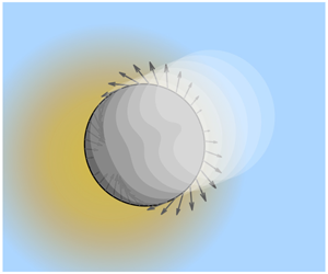
Figure 1. From diffusio-osmosis to diffusiophoresis: (a) schematic showing diffusio-osmotic flow generation. A surface (grey) is in contact with a gradient of solute (red particles). Here, the particles absorb on the surface creating a pressure in the fluid (represented by yellow arrows). This pressure build-up is stronger where the concentration is highest, and induces a hydrodynamic flow  $v_{DO}$ from the high concentration side to the low concentration side. (b) If this phenomenon occurs at the surface of a particle, the diffusio-osmotic flow will induce motion of the particle at a certain speed
  $v_{DP}$ in the opposite direction. This is called diffusiophoresis.
Interestingly, these phenomena have gained renewed interest over the last two decades, in particular thanks to the development of microfluidic technologies, which allow for an exquisite control of the physical conditions of the experiments, electric fields or concentration gradients. However, in contrast to electrophoresis, diffusiophoresis has been much less investigated since the pioneering work of Anderson and Prieve. Its amazing consequences in a broad variety of fields have only started to emerge, see Marbach & Bocquet (Reference Marbach and Bocquet2019) for a review and Abécassis et al. (Reference Abécassis, Cottin-Bizonne, Ybert, Ajdari and Bocquet2008), Palacci et al. (Reference Palacci, Abécassis, Cottin-Bizonne, Ybert and Bocquet2010, Reference Palacci, Cottin-Bizonne, Ybert and Bocquet2012), Velegol et al. (Reference Velegol, Garg, Guha, Kar and Kumar2016), Möller et al. (Reference Möller, Kriegel, Kieß, Sojo and Braun2017) and Shin, Warren & Stone (Reference Shin, Warren and Stone2018) for a few examples of applications. The diffusiophoretic velocity of a particle under a (dilute) solute gradient writes
 $$\begin{eqnarray}\boldsymbol{v}_{DP}=\unicode[STIX]{x1D707}_{DP}\times (-k_{B}T\unicode[STIX]{x1D735}c_{\infty }),\end{eqnarray}$$
 where  $\unicode[STIX]{x1D707}_{DP}$ is the diffusiophoretic mobility,
  $\unicode[STIX]{x1D735}c_{\infty }$ is the solute gradient far from the sphere,
  $k_{B}$ is Boltzmann’s constant and
  $T$ is temperature. For example, for a solute interacting with a spherical particle via a potential
  ${\mathcal{U}}(z)$, where
  $z$ is the distance to the particle surface, the diffusiophoretic mobility writes (Anderson & Prieve Reference Anderson and Prieve1991)
 $$\begin{eqnarray}\unicode[STIX]{x1D707}_{DP}=-\frac{1}{\unicode[STIX]{x1D702}}\int _{0}^{\infty }z\left(\exp \left(\frac{-{\mathcal{U}}(z)}{k_{B}T}\right)-1\right)\text{d}z.\end{eqnarray}$$
 In this work, we raise the question of the local and global force balance in phoretic phenomena, focusing in particular on diffusiophoresis. Indeed, while such interfacially driven motions are force free, i.e. the global force on the particle is zero, the local force balance is by no means obvious. For electrophoresis, it was discussed by Long, Viovy & Ajdari (Reference Long, Viovy and Ajdari1996) that local electroneutrality ensures that the force acting on the particle also vanishes locally in the case of a thin diffuse layer. Indeed, the force acting on the particle is the sum of the electric force  $dq\times \boldsymbol{E}_{loc}$, with
  $dq$ the charge on an elementary surface and
  $\boldsymbol{E}_{loc}$ the local electric field, and the hydrodynamic surface stress due to the electro-osmotic flow. To ensure mechanical balance within the electric double layer, this hydrodynamic stress has to be equal to the electric force on the double layer, which is exactly
  $-dq\,\boldsymbol{E}_{loc}$ since the electric double layer carries an opposite charge to the surface. Therefore, the local force on the particle surface vanishes. The absence of local force has some important consequences, among which we have the fact that particles such as polyelectrolytes undergoing electrophoresis do not deform under the action of the electric field (Long et al. Reference Long, Viovy and Ajdari1996).
Such arguments do not obviously extend to diffusiophoresis. The main physical reason is that diffusiophoresis involves the balance of viscous shearing with an osmotic pressure gradient acting in the diffuse layer along the particle surface (Marbach & Bocquet Reference Marbach and Bocquet2019). While such a balance is simple and appealing, it led to various mis-interpretations and debates concerning osmotically driven transport of particles (Córdova-Figueroa & Brady Reference Córdova-Figueroa and Brady2008, Reference Córdova-Figueroa and Brady2009a,Reference Córdova-Figueroa and Bradyb; Fischer & Dhar Reference Fischer and Dhar2009; Jülicher & Prost Reference Jülicher and Prost2009; Brady Reference Brady2011), also in the context of phoretic self-propulsion (Moran & Posner Reference Moran and Posner2017). A naive interpretation of diffusiophoresis is that the particle velocity  $v_{DP}$ results from the balance of Stokes’ viscous force
  $F_{v}=6\unicode[STIX]{x03C0}\unicode[STIX]{x1D702}Rv_{DP}$ and the osmotic force resulting from the osmotic pressure gradient integrated over the particle surface. The latter scales hypothetically as
  $F_{osm}\sim R^{2}\times R\unicode[STIX]{x1D735}\unicode[STIX]{x1D6F1}$, with
  $\unicode[STIX]{x1D6F1}=k_{B}Tc_{\infty }$ the osmotic pressure. Balancing the two forces, one predicts a phoretic velocity behaving as
  $v_{DP}\sim R^{2}(k_{B}T/\unicode[STIX]{x1D702})\unicode[STIX]{x1D735}c_{\infty }$. Looking at the expression for the diffusiophoretic mobility in the thin layer limit, equations (1.2) and (1.3), the latter argument does not match the previous estimate by a factor of order
  $(R/\unicode[STIX]{x1D706})^{2}$, where
  $\unicode[STIX]{x1D706}$ is the range of the potential of interaction between the solute and the particle. The reason why such a global force balance argument fails is that flows and interactions in interfacial transport occur typically over the thickness of the diffuse layer, in contradiction to the naive estimate above.
A second aspect which results from the previous argument is that the interplay between hydrodynamic stress and the osmotic pressure gradient for diffusiophoresis may lead to a non-vanishing local surface force. Indeed, in the absence of an electric force, only viscous shearing acts tangentially on the particle itself, while particle–solute neutral interactions mostly act in the orthogonal direction. A force tension may therefore be generated locally at the surface of the particle. This is in contrast to electrophoresis.
The question of global and local force balance in diffusiophoretic transport is therefore subtle and there is a need to clarify the mechanisms at stake. In the derivations below we first relax the hypothesis of a thin diffuse layer, and consider more explicitly the transport inside the diffuse layer, as was explored by various authors, using, for example, controlled asymptotic expansions (Sabass & Seifert Reference Sabass and Seifert2012; Córdova-Figueroa, Brady & Shklyaev Reference Córdova-Figueroa, Brady and Shklyaev2013; Sharifi-Mood, Koplik & Maldarelli Reference Sharifi-Mood, Koplik and Maldarelli2013). Then, on the basis of this general formulation, we are able to write properly the global and local force balance for diffusiophoresis. Our results confirm the existence of a non-vanishing surface stress in diffusiophoresis, in spite of the global force being zero. To illustrate the underlying mechanisms, we consider a number of cases: diffusiophoresis under a gradient of neutral solutes, diffusiophoresis of a charged particle in an electrolyte bath and diffusiophoresis of a porous particle. We also consider the situation of electrophoresis as a benchmark where the surface force on the particle is expected to vanish. We summarize our results in the next section and report the detailed calculations in the sections hereafter.
2 Geometry of the problem and main results: surface forces on a phoretic particle
2.1 Diffusiophoretic velocity
We consider a sphere of radius  $R$ in a solution containing one or multiple solutes, charged or not. The surface of the sphere interacts with the species over a typical length scale
  $\unicode[STIX]{x1D706}$, via, for example, electric interactions, steric repulsion or any other interaction. In the case of diffusiophoresis, a gradient of solute,
  $\unicode[STIX]{x1D735}c_{\infty }$, is established at infinity along the direction
  $z$ – see figure 2 for a schematic in the diffusiophoretic case. The sphere moves accordingly at constant velocity
  $v_{DP}\boldsymbol{e}_{z}$ and we place ourselves in the sphere’s frame of reference. We consider that the interaction between the solute and the particle occurs via a potential
  ${\mathcal{U}}$, so that Stokes’ equation for the fluid surrounding the sphere writes
 $$\begin{eqnarray}\unicode[STIX]{x1D702}\unicode[STIX]{x1D6FB}^{2}\boldsymbol{v}-\unicode[STIX]{x1D735}p+c(\boldsymbol{r})(-\unicode[STIX]{x1D735}{\mathcal{U}})=0.\end{eqnarray}$$
The latter term of the Stokes equation (2.1) corresponds to the action of the particle on the fluid (the fluid is constituted of the solvent and the solute). Formulation of osmotic related effects with this kinetic approach can be found in Debye (Reference Debye1923), Manning (Reference Manning1968), Anderson, Lowell & Prieve (Reference Anderson, Lowell and Prieve1982), Marbach, Yoshida & Bocquet (Reference Marbach, Yoshida and Bocquet2017) and Marbach & Bocquet (Reference Marbach and Bocquet2019). The boundary conditions on the particle’s surface are the no-slip boundary condition (note that the no-slip boundary condition may be relaxed to account for partial slip at the surface, in line with Ajdari & Bocquet (Reference Ajdari and Bocquet2006)), complemented by the prescribed velocity at infinity (in the frame of reference of the particle)
 $$\begin{eqnarray}\boldsymbol{v}(r=R)=\mathbf{0}\quad \text{and}\quad \boldsymbol{v}(r\rightarrow \infty )=-\boldsymbol{v}_{DP}.\end{eqnarray}$$
 The solute concentration profile obeys a Smoluchowski equation in the presence of the external potential  ${\mathcal{U}}$, in the form
 $$\begin{eqnarray}0=-\unicode[STIX]{x1D735}\boldsymbol{\cdot }\left[-D_{s}\unicode[STIX]{x1D735}c+\frac{D_{s}}{k_{B}T}c(-\unicode[STIX]{x1D735}{\mathcal{U}})\right],\end{eqnarray}$$
 where  $D_{s}$ is the diffusion coefficient of the solute, with the boundary condition at infinity accounting for a constant solute gradient
  $c(r\rightarrow \infty )\simeq c_{0}+r\cos \unicode[STIX]{x1D703}\unicode[STIX]{x1D735}c_{\infty }$;
  $c_{0}$ is a reference concentration and
  $\unicode[STIX]{x1D703}$ the angle between the
  $z$ axis along which the particle moves and the radial axis – see figure 2. Note that we have neglected convective transport here, assuming a low Péclet regime. The Péclet number here may be defined as
  $Pe=v_{DP}R/D_{s}$ (see, e.g. Prieve et al. (Reference Prieve, Anderson, Ebel and Lowell1984)) where
  $R$ is the relevant length scale at which convection takes place. Using the typical expression for the diffusiophoretic velocity we have
  $v_{DP}=(k_{B}T/\unicode[STIX]{x1D702})\unicode[STIX]{x1D706}\unicode[STIX]{x1D6E4}\unicode[STIX]{x1D735}c_{\infty }$, where
  $\unicode[STIX]{x1D706}$ is the range of the interaction and
  $\unicode[STIX]{x1D6E4}$ is a length that measures the excess (or default) of solute near the interface. Using further Einstein’s formula
  $D_{s}\sim k_{B}T/6\unicode[STIX]{x03C0}\unicode[STIX]{x1D702}R_{s}$ (where
  $R_{s}$ is the hydrodynamic radius of the solute) the condition for small Péclet number then amounts to
  $6\unicode[STIX]{x03C0}(\unicode[STIX]{x1D6E4}/R)(\unicode[STIX]{x1D706}/R)(c_{0}R^{3})(R\unicode[STIX]{x1D735}c_{\infty }/c_{0})(R_{s}/R)\ll 1$. For reasonably sized colloids
  $R\sim 100~\text{nm}$ and with typical conditions
  $c_{0}\sim 10~\text{mM}$,
  $R_{s}\sim 0.1~\text{nm}$ we find
  $(\unicode[STIX]{x1D6E4}/R)(\unicode[STIX]{x1D706}/R)(R\unicode[STIX]{x1D735}c_{\infty }/c_{0})\lesssim 10^{-2}$. The length scale of the concentration gradient
  $c_{0}/\unicode[STIX]{x1D735}c_{\infty }$ is always larger than the size of the colloid, such that to work at low Péclet numbers we only need
  $(\unicode[STIX]{x1D6E4}/R)(\unicode[STIX]{x1D706}/R)$ to be rather small. This means that either the interaction strength is small (weak absorption, or weak potential) or the interaction layer is small
  $\unicode[STIX]{x1D706}\ll R$. As we do not wish to constrain the problem to either case, we simply assume
  $Pe\ll 1$ and do not make any detailed assumption on
  $\unicode[STIX]{x1D706}$ or the strength of the potential. Finally, the Smoluchowski equation is self-consistent and provides a solution for the solute concentration field (in full generality we may write the axisymmetric solution as
  $c(r,\unicode[STIX]{x1D703})=c_{0}+c_{0}(r)\cos \unicode[STIX]{x1D703}$), which therefore acts as an independent source term for the fluid equation of motion in (2.1). We further stress that taking into account convective transport does not affect the results at lowest order (O’Brien & White Reference O’Brien and White1978; Prieve et al. Reference Prieve, Anderson, Ebel and Lowell1984; Prieve & Roman Reference Prieve and Roman1987; Ajdari & Bocquet Reference Ajdari and Bocquet2006) and therefore the qualitative conclusions that we will draw on force balance here are not affected by this assumption.

Figure 2. Schematic of the coordinate system for the diffusiophoretic sphere. The sphere interacts with the solute via a potential  ${\mathcal{U}}(r)$ over a range
  $\unicode[STIX]{x1D706}$ not necessarily small compared to the radius of the sphere
  $R$.
$R$.
In this paper we report analytic results in various cases as represented in figure 3. First (see figure 3a), we show that, for any radially symmetric potential  ${\mathcal{U}}(r)$, one may compute an exact solution of (2.1) for the velocity profile and the local force. Second, going to more general electro-chemical drivings, like electrophoresis (see figure 3b) or diffusiophoresis of a charged sphere in an electrolyte solution (see figure 3c), it is also possible to compute exact solutions, assuming a weak driving force with respect to equilibrium. Finally, we come back to simple diffusiophoresis of a porous sphere with a radially symmetric potential
  ${\mathcal{U}}(r)$ (see figure 3d) and give similar analytic results. The porosity of the sphere is accounted for by allowing flow inside the sphere with a given permeability.

Figure 3. Geometries considered in this paper. (a) Diffusiophoresis under neutral solute gradients: a spherical particle moving in a (uncharged) solute gradient. (b) Electrophoresis: a spherical particle with surface charge  $\unicode[STIX]{x1D6F4}$ moving in an electric field in a uniform electrolyte. (c) Diffusiophoresis under ionic concentration gradients: a spherical particle with surface charge
  $\unicode[STIX]{x1D6F4}$ moving in an electrolyte gradient. (d) Diffusiophoresis of a porous particle: a porous spherical particle moving in an uncharged solute gradient.
2.2 Phoretic velocity
We summarize briefly the analytic results for the phoretic velocity in the various cases considered. Results are reported in table 1.
Table 1. Main results for the phoretic velocity of plain and porous colloidal particles. Here,  $\unicode[STIX]{x1D6FD}=1/k_{B}T$,
  $\tilde{\unicode[STIX]{x1D707}}_{i}$ is field which is the perturbation to the chemical potential of species
  $i$ under the applied field, i.e.
  $\tilde{\unicode[STIX]{x1D707}}_{i}\propto \unicode[STIX]{x1D735}\unicode[STIX]{x1D707}_{\infty }$ the applied electro-chemical gradient at infinity;
  $\unicode[STIX]{x1D70C}_{0,i}$ is the concentration profile of species
  $i$ in equilibrium.

a Note that this result is similar to the diffusio-osmotic velocity over a plane surface reported in Anderson & Prieve (Reference Anderson and Prieve1991).
Diffusiophoresis under gradients of a neutral solute. For any radially symmetric potential  ${\mathcal{U}}(r)$, one may compute an exact solution of (2.1) for the velocity profile by extending textbook techniques for the Stokes problem in Happel & Brenner (Reference Happel and Brenner2012) (see also Ohshima, Healy & White (Reference Ohshima, Healy and White1983) for a related calculation in the context of electrophoresis). It can be demonstrated that the solution for
  $\boldsymbol{v}(\boldsymbol{r})$ involves a Stokeslet as a leading term, which allows us to calculate the force along the axis of the gradient as the prefactor of the Stokeslet term (
 $v\sim F/r$). This allows us to deduce the global force on the particle as
 $$\begin{eqnarray}F=6\unicode[STIX]{x03C0}R\unicode[STIX]{x1D702}v_{DP}-2\unicode[STIX]{x03C0}R^{2}\int _{R}^{\infty }c_{0}(r)(-\unicode[STIX]{x2202}_{r}{\mathcal{U}})(r)\times \unicode[STIX]{x1D711}(r)\,\text{d}r,\end{eqnarray}$$
 with  $\unicode[STIX]{x1D711}(r)=r/R-R/3r-\frac{2}{3}(r/R)^{2}$ a dimensionless function, the factor
  $\frac{2}{3}$ originating from the angular average, and the function
  $c_{0}(r)$ is such that the concentration profile writes
  $c(r,\unicode[STIX]{x1D703})=c_{0}+c_{0}(r)\cos \unicode[STIX]{x1D703}$. Equation (2.4) decomposes as the sum of the classic Stokes friction force on the sphere and a balancing force of osmotic origin, taking its root in the interaction
  ${\mathcal{U}}$ of the solute with the particle. The steady-state diffusiophoretic velocity results from the force-free condition,
  $F=0$, and therefore writes
 $$\begin{eqnarray}v_{DP}=\frac{2\unicode[STIX]{x03C0}R^{2}}{6\unicode[STIX]{x03C0}\unicode[STIX]{x1D702}R}\int _{R}^{\infty }c_{0}(r)(-\unicode[STIX]{x2202}_{r}{\mathcal{U}})(r)\times \unicode[STIX]{x1D711}(r)\,\text{d}r.\end{eqnarray}$$
 Remembering that  $c_{0}(r)\propto R\unicode[STIX]{x1D735}c_{\infty }$, this equation generalizes (1.2) obtained in the thin layer limit. Note that (2.5) is very similar to (2.7) in Brady (Reference Brady2011), with the
  $r$-dependent term
  $2\unicode[STIX]{x03C0}R^{2}\times \unicode[STIX]{x1D711}(r)$ replaced in Brady (Reference Brady2011) by the prefactor
  $L(R)$. However, the integrated ‘osmotic push’ is weighted here by the local factor
  $\unicode[STIX]{x1D711}(r)$ (in contrast to Brady (Reference Brady2011)) and this detail actually changes the whole scaling for the mobility.
Generalized formula for phoresis under electro-chemical gradients. It is possible to generalize the previous results to charged species under an electro-chemical potential gradient. The general expression for the diffusiophoretic velocity is written in terms of the electro-chemical potential  $\unicode[STIX]{x1D707}_{i}$ (where
  $i$ stands for each solute species
  $i$). One may separate the electro-chemical potential as
  $\unicode[STIX]{x1D707}_{i}=\unicode[STIX]{x1D707}_{0,i}+\tilde{\unicode[STIX]{x1D707}}_{i}$, where
  $\unicode[STIX]{x1D707}_{0,i}$ is the equilibrium chemical potential and
  $\tilde{\unicode[STIX]{x1D707}}_{i}$ the perturbation due to an external field, so that
  $\tilde{\unicode[STIX]{x1D707}}_{i}\propto \unicode[STIX]{x1D735}\unicode[STIX]{x1D707}_{\infty }$, the applied electro-chemical potential gradient at infinity. The derivation assumes a weak perturbation,
  $\tilde{\unicode[STIX]{x1D707}}_{i}\ll \unicode[STIX]{x1D707}_{0,i}$. This leads to an expression of the generalized expression for the diffusiophoretic velocity in a compact form
 $$\begin{eqnarray}\displaystyle v_{P}=\frac{R}{3\unicode[STIX]{x1D702}}\int _{R}^{\infty }\left(\mathop{\sum }_{species\,i}\unicode[STIX]{x2202}_{r}\unicode[STIX]{x1D70C}_{0,i}\times \tilde{\unicode[STIX]{x1D707}}_{i}\right)\unicode[STIX]{x1D711}(r)\,\text{d}r,\end{eqnarray}$$
 where  $\unicode[STIX]{x1D70C}_{0,i}$ is the concentration profile at equilibrium. Details of the calculations are reported in § 4.
Diffusiophoresis of a porous sphere. It is possible to extend the derivation to the case of a porous colloid. This may be considered as a coarse-grained model for a polymer. We assume in this case that the solute is neutral and interacts with the sphere via a radially symmetric potential  ${\mathcal{U}}$. In that case the Stokes equation (2.1) is extended inside the porous sphere with the addition of a Darcy term
 $$\begin{eqnarray}\unicode[STIX]{x1D702}\unicode[STIX]{x1D6FB}^{2}\boldsymbol{v}-\frac{\unicode[STIX]{x1D702}}{\unicode[STIX]{x1D705}}\boldsymbol{v}-\unicode[STIX]{x1D735}p+c(\boldsymbol{r})(-\unicode[STIX]{x1D735}{\mathcal{U}})=0,\end{eqnarray}$$
 where  $\unicode[STIX]{x1D705}$, expressed in units of a length squared, is the permeability of the sphere. The expression for the diffusiophoretic velocity can be calculated explicitly, with an expression formally similar to the diffusiophoretic velocity,
 $$\begin{eqnarray}v_{DP,p}=\frac{R}{3\unicode[STIX]{x1D702}}\int _{0}^{\infty }\frac{c(r,\unicode[STIX]{x1D703})-c_{0}}{\cos \unicode[STIX]{x1D703}}(-\unicode[STIX]{x2202}_{r}{\mathcal{U}})\unicode[STIX]{x1D6F7}(r)\,\text{d}r,\end{eqnarray}$$
 where the details of the porous nature of the colloid are accounted for in the weight  $\unicode[STIX]{x1D6F7}(r)$, as reported in (5.18). The latter is a complex function of
  $k_{\unicode[STIX]{x1D705}}R$, where
  $k_{\unicode[STIX]{x1D705}}=1/\sqrt{\unicode[STIX]{x1D705}}$ is the inverse screening length associated with the permeability of the colloid, with radius
  $R$. Details of the calculations are reported in § 5.
2.3 Local force balance on the surface
Beyond the diffusiophoretic velocity, the theoretical framework also allows us to compute the global and local forces on the particle. Writing the local force balance at the particle surface, we find in general that the particle withstands a local force that does not vanish for diffusiophoresis. The local force  $\text{d}\boldsymbol{f}$ on an element of surface
  $\text{d}S$ of a phoretic particle can be written generally as
 $$\begin{eqnarray}\text{d}\boldsymbol{f}=\left(-p_{0}+{\textstyle \frac{2}{3}}\unicode[STIX]{x03C0}_{s}\cos \unicode[STIX]{x1D703}\right)\text{d}S\boldsymbol{e}_{r}+\left({\textstyle \frac{1}{3}}\unicode[STIX]{x03C0}_{s}\sin \unicode[STIX]{x1D703}\right)\text{d}S\boldsymbol{e}_{\unicode[STIX]{x1D703}},\end{eqnarray}$$
 where the local force is fully characterized by a force per unit area – or pressure –  $\unicode[STIX]{x03C0}_{s}$. In this expression
  $p_{0}$ is the bulk hydrostatic pressure and
  $\boldsymbol{e}_{r}$ and
  $\boldsymbol{e}_{\unicode[STIX]{x1D703}}$ are the unit vectors in the spherical coordinate system centred on the sphere. We report the value of
  $\unicode[STIX]{x03C0}_{s}$ in the table below for the various cases considered, see table 2. While the surface force is found to be non-vanishing for all diffusiophoretic transport, our calculations show that
  $\unicode[STIX]{x03C0}_{s}\equiv 0$ for electrophoretic driving: a local force balance is predicted for electrophoresis in agreement with the argument of in Long et al. (Reference Long, Viovy and Ajdari1996) (see the details in § 4).
Table 2. Main results for the local surface force on plain and porous colloidal particles undergoing phoretic transport. Here,  $\unicode[STIX]{x1D6FD}=1/k_{B}T$,
  $\tilde{\unicode[STIX]{x1D707}}_{i}$ is the perturbation to the chemical potential of species
  $i$ and
  $\unicode[STIX]{x1D70C}_{0,i}$ its concentration profile in equilibrium. Note that
  $\unicode[STIX]{x1D706}_{D}$ is the Debye length (
 $\unicode[STIX]{x1D706}_{D}^{-2}=e^{2}c_{0}/\unicode[STIX]{x1D716}k_{B}T$) and
  $Du=\unicode[STIX]{x1D6F4}/e\unicode[STIX]{x1D706}_{D}c_{0}$ is a Dukhin number.

Let us report more specifically the results for the local force in the different cases.
Local force for diffusiophoresis with neutral solutes. For solutes interacting with the colloid via a soft interaction potential  ${\mathcal{U}}(r)$, one finds that the surface force takes the form
 $$\begin{eqnarray}\unicode[STIX]{x03C0}_{s}=\int _{R}^{\infty }c_{0}(r)(-\unicode[STIX]{x2202}_{r}{\mathcal{U}})(r)\unicode[STIX]{x1D713}(r)\,\text{d}r,\end{eqnarray}$$
 where  $\unicode[STIX]{x1D713}(r)=R/r-r^{2}/R^{2}$ is a geometrical factor. As we demonstrate in the following sections, in the case of a thin double layer, the local force reduces to a simple and transparent expression
 $$\begin{eqnarray}\unicode[STIX]{x03C0}_{s}\simeq {\textstyle \frac{9}{2}}k_{B}TL_{s}\unicode[STIX]{x1D735}c_{\infty },\end{eqnarray}$$
 where  $L_{s}=\int _{R}^{\infty }(\text{e}^{-\unicode[STIX]{x1D6FD}{\mathcal{U}}(z)}-1)\,\text{d}z$ has the dimension of a length and quantifies the excess adsorption on the interface, and
  $\unicode[STIX]{x1D6FD}=1/k_{B}T$.
Local force for phoresis under small electro-chemical gradients. As for the velocity, it is possible to generalize the previous results to the case of a general, small, electro-chemical driving. In the case of a thin diffuse layer, the result for  $\unicode[STIX]{x03C0}_{s}$ takes the generic form
 $$\begin{eqnarray}\displaystyle \unicode[STIX]{x03C0}_{s}=\int _{R}^{\infty }\left(\mathop{\sum }_{species\,i}\unicode[STIX]{x2202}_{r}\unicode[STIX]{x1D70C}_{0,i}\times \tilde{\unicode[STIX]{x1D707}}_{i}\right)\unicode[STIX]{x1D713}(r)\,\text{d}r,\end{eqnarray}$$
 with  $\unicode[STIX]{x1D713}(r)=R/r-r^{2}/R^{2}$ and we recall that
  $\tilde{\unicode[STIX]{x1D707}}_{i}\propto \unicode[STIX]{x1D735}\unicode[STIX]{x1D707}_{\infty }$ the gradient of the electro-chemical potential far from the colloid. This result applies to both diffusio- and electro-phoresis. As reported in table 2, the local force is non-vanishing for diffusiophoresis but for electrophoresis one predicts
  $\unicode[STIX]{x03C0}_{s}\equiv 0$.
Local force for diffusiophoresis of a porous particle. Finally, for a porous colloid undergoing diffusiophoresis, the local force is a function of the permeability and the diffusion coefficient of the solute inside and outside the colloid, say  $D_{1}$ and
  $D_{2}$. The general formula writes as
 $$\begin{eqnarray}\unicode[STIX]{x03C0}_{s}=\int _{R}^{+\infty }\frac{c(r,\unicode[STIX]{x1D703})-c_{0}}{\cos \unicode[STIX]{x1D703}}\unicode[STIX]{x2202}_{r}(-{\mathcal{U}})\unicode[STIX]{x1D6F9}(r)\,\text{d}r,\end{eqnarray}$$
 where the expression for the function  $\unicode[STIX]{x1D6F9}(r)$ is given in (5.24). This is a quite cumbersome expression in general, but in the thin diffuse layer limit, and with small permeability
  $\unicode[STIX]{x1D705}$ of the colloid, the local force takes a simple form
 $$\begin{eqnarray}\unicode[STIX]{x03C0}_{s}(\unicode[STIX]{x1D705}\rightarrow 0)=\unicode[STIX]{x03C0}_{s}(\unicode[STIX]{x1D705}=0)\times \frac{D_{2}}{D_{2}+D_{1}/2}\left(1-\frac{2}{k_{\unicode[STIX]{x1D705}}R}\right),\end{eqnarray}$$
 where  $\unicode[STIX]{x03C0}_{s}(\unicode[STIX]{x1D705}=0)=\frac{9}{2}L_{s}k_{B}T\unicode[STIX]{x1D735}c_{\infty }$;
  $k_{\unicode[STIX]{x1D705}}=1/\sqrt{\unicode[STIX]{x1D705}}$ is the inverse screening length associated with the Darcy flow inside the porous colloid, and
  $R$ is the particle radius.
In the next sections we detail the calculations leading to the results in tables 1 and 2.
3 Diffusiophoresis of a colloid under a gradient of neutral solute
We focus first on diffusiophoresis of an impermeable particle, see figure 3(a), under a concentration gradient of neutral solute. The solute interacts with the particle via a soft interaction potential  ${\mathcal{U}}(r)$ which only depends on the radial coordinate
  $r$ (with the origin at the sphere centre). In order to simplify the calculations, we will consider that the interaction potential is non-zero only over a finite range, from the surface of the sphere
  $r=R$ to some boundary layer
  $r=R+\unicode[STIX]{x1D706}$: the range
  $\unicode[STIX]{x1D706}$ is finite but not necessarily small as compared to
  $R$, see figure 2. One may take
  $\unicode[STIX]{x1D706}\rightarrow \infty$ at the end of the calculation.
In the far field, the solute concentration obeys  $\unicode[STIX]{x1D735}c|_{r\rightarrow \infty }=\unicode[STIX]{x1D735}c_{\infty }\boldsymbol{e}_{z}$. The geometry is axisymmetric, and thus in spherical coordinates one may write
  $c(r\rightarrow \infty ,\unicode[STIX]{x1D703})=c_{0}+\unicode[STIX]{x1D735}c_{\infty }r\cos \unicode[STIX]{x1D703}$. Considering the boundary conditions for the concentration and the symmetry of the potential
  ${\mathcal{U}}$, one expects that the concentration distribution in the radial coordinate
  $r$ and the polar angle
  $\unicode[STIX]{x1D703}$ can be written as
  $c(r,\unicode[STIX]{x1D703})=c_{0}+R\unicode[STIX]{x1D735}c_{\infty }\times f(r)\cos \unicode[STIX]{x1D703}$, where
  $f(r)$ is a radial and dimensionless function, which remains to be calculated.
Note that in the following we neglect convection of the solute within the interfacial region, which may modify the steady-state concentration field of the solute around the particle. However, such an assumption is generally valid because the Péclet number built on the diffuse layer is expected to be small. Our results could, however, be extended to include this effect on the mobility as a function of a (properly defined) Péclet number, as introduced in Anderson & Prieve (Reference Anderson and Prieve1991), Ajdari & Bocquet (Reference Ajdari and Bocquet2006), Sabass & Seifert (Reference Sabass and Seifert2012) and Michelin & Lauga (Reference Michelin and Lauga2014). Similarly, the effect of hydrodynamic fluid slippage at the particle surface may be taken into account, in line with the description in Ajdari & Bocquet (Reference Ajdari and Bocquet2006).
3.1 Flow profile
3.1.1 Constitutive equations for the flow profile
The flow profile around the sphere is incompressible  $\text{div}(\boldsymbol{v})=0$ and obeys Stokes’ equation, equation (2.1). The projection of the Stokes equation along the unit vectors
  $\boldsymbol{e}_{r}$ and
  $\boldsymbol{e}_{\unicode[STIX]{x1D703}}$ gives
 $$\begin{eqnarray}\left.\begin{array}{@{}c@{}}\displaystyle \unicode[STIX]{x1D702}\left(\unicode[STIX]{x0394}v_{r}-\frac{2v_{r}}{r^{2}}-2\frac{v_{\unicode[STIX]{x1D703}}\cos \unicode[STIX]{x1D703}}{r^{2}\sin \unicode[STIX]{x1D703}}-\frac{2}{r^{2}}\frac{\unicode[STIX]{x2202}v_{\unicode[STIX]{x1D703}}}{\unicode[STIX]{x2202}\unicode[STIX]{x1D703}}\right)=\unicode[STIX]{x2202}_{r}p-c(r,\unicode[STIX]{x1D703})\unicode[STIX]{x2202}_{r}(-{\mathcal{U}}),\\ \displaystyle \unicode[STIX]{x1D702}\left(\unicode[STIX]{x0394}v_{\unicode[STIX]{x1D703}}-\frac{v_{\unicode[STIX]{x1D703}}}{r^{2}\sin ^{2}\unicode[STIX]{x1D703}}+\frac{2}{r^{2}}\frac{\unicode[STIX]{x2202}v_{r}}{\unicode[STIX]{x2202}\unicode[STIX]{x1D703}}\right)=\frac{1}{r}\unicode[STIX]{x2202}_{\unicode[STIX]{x1D703}}p.\end{array}\right\}\end{eqnarray}$$
The boundary conditions for the flow are (i) the prescribed diffusiophoretic flow far from the sphere, and (ii) impermeability and no-slip condition on the particle surface
 $$\begin{eqnarray}\left.\begin{array}{@{}c@{}}v_{r}(r\rightarrow \infty ,\unicode[STIX]{x1D703})=-v_{DP}\cos \unicode[STIX]{x1D703}\quad \text{and}\quad v_{\unicode[STIX]{x1D703}}(r\rightarrow \infty ,\unicode[STIX]{x1D703})=v_{DP}\sin \unicode[STIX]{x1D703},\\ v_{r}(r=R,\unicode[STIX]{x1D703})=0\quad \text{and}\quad v_{\unicode[STIX]{x1D703}}(r=R,\unicode[STIX]{x1D703})=0.\end{array}\right\}\end{eqnarray}$$
3.1.2 Solution for the flow profile
We define a potential field  $\unicode[STIX]{x1D713}$ such that
 $$\begin{eqnarray}v_{r}=\frac{1}{r^{2}\sin \unicode[STIX]{x1D703}}\unicode[STIX]{x2202}_{\unicode[STIX]{x1D703}}\unicode[STIX]{x1D713}\quad \text{and}\quad v_{\unicode[STIX]{x1D703}}=-\frac{1}{r\sin \unicode[STIX]{x1D703}}\unicode[STIX]{x2202}_{r}\unicode[STIX]{x1D713}\end{eqnarray}$$
 so that the incompressibility condition  $\text{div}(\boldsymbol{v})=0$ is accordingly verified. We can rewrite the Stokes equations using the operator
  $E^{2}=\unicode[STIX]{x2202}^{2}/\unicode[STIX]{x2202}r^{2}+(\sin \unicode[STIX]{x1D703}/r^{2})(\unicode[STIX]{x2202}/\unicode[STIX]{x2202}\unicode[STIX]{x1D703})((1/\sin \unicode[STIX]{x1D703})(\unicode[STIX]{x2202}/\unicode[STIX]{x2202}\unicode[STIX]{x1D703}))$ as
 $$\begin{eqnarray}\left.\begin{array}{@{}c@{}}\displaystyle \frac{\unicode[STIX]{x1D702}}{r^{2}\sin \unicode[STIX]{x1D703}}\unicode[STIX]{x2202}_{\unicode[STIX]{x1D703}}[E^{2}\unicode[STIX]{x1D713}]=\unicode[STIX]{x2202}_{r}p-c(r,\unicode[STIX]{x1D703})\unicode[STIX]{x2202}_{r}(-{\mathcal{U}}),\\ \displaystyle \frac{-\unicode[STIX]{x1D702}}{r\sin \unicode[STIX]{x1D703}}\unicode[STIX]{x2202}_{r}[E^{2}\unicode[STIX]{x1D713}]=\frac{1}{r}\unicode[STIX]{x2202}_{\unicode[STIX]{x1D703}}p.\end{array}\right\}\end{eqnarray}$$
Adding up derivatives of the above formula allows us to cancel the pressure contribution and obtain the simple equation for the potential field
 $$\begin{eqnarray}\unicode[STIX]{x1D702}E^{4}\unicode[STIX]{x1D713}=-\text{sin}\,\unicode[STIX]{x1D703}\frac{\unicode[STIX]{x2202}c(r,\unicode[STIX]{x1D703})}{\unicode[STIX]{x2202}\unicode[STIX]{x1D703}}\unicode[STIX]{x2202}_{r}(-{\mathcal{U}}).\end{eqnarray}$$
 Using the general expression for  $c(r,\unicode[STIX]{x1D703})=c_{0}+c_{0}(r)\cos \unicode[STIX]{x1D703}$ where we may rewrite
  $c_{0}(r)=R\unicode[STIX]{x1D735}c_{\infty }f(r)$, one obtains
 $$\begin{eqnarray}\unicode[STIX]{x1D702}E^{4}\unicode[STIX]{x1D713}=\sin ^{2}\unicode[STIX]{x1D703}R\unicode[STIX]{x1D735}c_{\infty }\,f(r)\unicode[STIX]{x2202}_{r}(-{\mathcal{U}}).\end{eqnarray}$$
 We may therefore look for  $\unicode[STIX]{x1D713}$ as
  $\unicode[STIX]{x1D713}=F(r)\sin ^{2}\unicode[STIX]{x1D703}$ and we note that
  $E^{2}\unicode[STIX]{x1D713}=\tilde{E}^{2}F(r)\sin ^{2}\unicode[STIX]{x1D703}$, where
  $\tilde{E}^{2}=\unicode[STIX]{x2202}^{2}/\unicode[STIX]{x2202}r^{2}-2/r^{2}$ so that
 $$\begin{eqnarray}\tilde{E}^{4}F(r)=\frac{\unicode[STIX]{x1D735}c_{\infty }R}{\unicode[STIX]{x1D702}}f(r)\unicode[STIX]{x2202}_{r}(-{\mathcal{U}}).\end{eqnarray}$$
 We introduce  $\tilde{f}(r)=(\unicode[STIX]{x1D735}c_{\infty }R/\unicode[STIX]{x1D702})f(r)\unicode[STIX]{x2202}_{r}(-{\mathcal{U}})$. Like the potential
  ${\mathcal{U}}(r)$,
  $\tilde{f}(r)$ is a compact function that is non-zero only over the interval
  $[R;R+\unicode[STIX]{x1D706}]$. The general solution of this equation is
 $$\begin{eqnarray}\displaystyle F(r) & = & \displaystyle \frac{A}{r}+Br+r^{2}C+Dr^{4}-\frac{1}{r}\int _{R}^{r}\frac{\tilde{f}(x)x^{4}}{30}\,\text{d}x+r\int _{R}^{r}\frac{\tilde{f}(x)x^{2}}{6}\,\text{d}x\nonumber\\ \displaystyle & & \displaystyle -\,r^{2}\int _{R}^{r}\frac{\tilde{f}(x)x}{6}\,\text{d}x+r^{4}\int _{R}^{r}\frac{\tilde{f}(x)}{30x}\,\text{d}x,\end{eqnarray}$$
 where  $A,B,C$ and
  $D$ are integration constants to be determined by the boundary conditions. Note that the integrals do not diverge since
  $\tilde{f}$ is defined on a compact interval. The condition that the flow has to be finite far from the sphere
  $r\rightarrow \infty$ yields immediately
 $$\begin{eqnarray}D=-\int _{R}^{R+\unicode[STIX]{x1D706}}\frac{\tilde{f}(x)}{30x}\,\text{d}x\quad \text{and}\quad C=\int _{R}^{R+\unicode[STIX]{x1D706}}\frac{\tilde{f}(x)x}{6}\,\text{d}x-\frac{v_{DP}}{2}.\end{eqnarray}$$
 Impermeability and no-slip boundary conditions are equivalent to  $F(R)=F^{\prime }(R)=0$. This gives the values of
  $A$ and
  $B$ and the flow is now fully specified as
 $$\begin{eqnarray}\left.\begin{array}{@{}c@{}}\displaystyle F(r)=\frac{A}{r}+Br-\frac{r^{2}}{2}v_{DP}+\int _{R}^{r}\tilde{f}(x)\left(\frac{rx^{2}}{6}-\frac{x^{4}}{30r}\right)\text{d}x+\int _{R+\unicode[STIX]{x1D706}}^{r}\tilde{f}(x)\left(\frac{r^{4}}{30x}-r^{2}\frac{x}{6}\right)\text{d}x\\ \displaystyle \text{with}\quad A=-\frac{R^{3}}{4}v_{DP}+\int _{R}^{R+\unicode[STIX]{x1D706}}\tilde{f}(x)\left(\frac{R^{3}x}{12}-\frac{R^{5}}{20x}\right)\text{d}x\\ \displaystyle \text{and}\quad B=\frac{3R}{4}v_{DP}+\int _{R}^{R+\unicode[STIX]{x1D706}}\tilde{f}(x)\left(\frac{R^{3}}{12x}-\frac{Rx}{4}\right)\text{d}x.\end{array}\right\}\end{eqnarray}$$
This provides an explicit expression for the flow profile as
 $$\begin{eqnarray}\left.\begin{array}{@{}c@{}}\displaystyle v_{r}=\sin \unicode[STIX]{x1D703}\left(2\frac{\tilde{B}(r)}{r}+\frac{2\tilde{A}(r)}{r^{3}}+2\tilde{C}(r)+2\tilde{D}(r)r^{2}\right),\\ \displaystyle v_{\unicode[STIX]{x1D703}}=\cos \unicode[STIX]{x1D703}\left(-\frac{\tilde{B}(r)}{r}+\frac{\tilde{A}(r)}{r^{3}}-2\tilde{C}(r)-4\tilde{D}(r)r\right).\end{array}\right\}\end{eqnarray}$$
 Analytical expressions can be obtained for all coefficients but we report here only the expression for  $\tilde{B}$:
 $$\begin{eqnarray}\tilde{B}(r)=B+\int _{R}^{r}\frac{1}{6}\,\tilde{f}(x)x^{2}\,\text{d}x.\end{eqnarray}$$
 This is the coefficient in front of the Stokeslet term, scaling as  $1/r$, hence directly related to the force acting on the particle. As we discuss below, the diffusiophoretic velocity is deduced from the force-free condition, which amounts to writing
  $\tilde{B}(r\rightarrow \infty )=0$.
3.2 Forces on the sphere
3.2.1 Pressure field and hydrodynamic force
The pressure field  $p$ can be computed from its full derivative
 $$\begin{eqnarray}\text{d}p=\unicode[STIX]{x2202}_{r}p\,\text{d}r+\unicode[STIX]{x2202}_{\unicode[STIX]{x1D703}}p\,\text{d}\unicode[STIX]{x1D703}.\end{eqnarray}$$
Using (3.4) and (3.5) we can integrate the pressure field and find
 $$\begin{eqnarray}p=p_{0}+\unicode[STIX]{x1D702}\cos \unicode[STIX]{x1D703}\unicode[STIX]{x2202}_{r}[\tilde{E}^{2}F(r)].\end{eqnarray}$$
The components of the hydrodynamic stress can be written as
 $$\begin{eqnarray}\left.\begin{array}{@{}c@{}}\displaystyle \unicode[STIX]{x1D70E}_{rr}=-p+2\unicode[STIX]{x1D702}\frac{\unicode[STIX]{x2202}v_{r}}{\unicode[STIX]{x2202}r},\\ \displaystyle \unicode[STIX]{x1D70E}_{r\unicode[STIX]{x1D703}}=\unicode[STIX]{x1D702}\left(\frac{1}{r}\frac{\unicode[STIX]{x2202}v_{r}}{\unicode[STIX]{x2202}\unicode[STIX]{x1D703}}+\frac{\unicode[STIX]{x2202}v_{\unicode[STIX]{x1D703}}}{\unicode[STIX]{x2202}r}-\frac{v_{\unicode[STIX]{x1D703}}}{r}\right).\end{array}\right\}\end{eqnarray}$$
This leads to the expression for the normal and tangential hydrodynamic forces as
 $$\begin{eqnarray}\frac{\text{d}f_{r}^{hydro}}{\text{d}S}=\unicode[STIX]{x1D70E}_{rr}|_{r=R}=-p_{0}-\unicode[STIX]{x1D702}\cos \unicode[STIX]{x1D703}\unicode[STIX]{x2202}_{rrr}F(r)|_{r=R}\end{eqnarray}$$
and
 $$\begin{eqnarray}\frac{\text{d}f_{\unicode[STIX]{x1D703}}^{hydro}}{\text{d}S}=\unicode[STIX]{x1D70E}_{r\unicode[STIX]{x1D703}}|_{r=R}=-\unicode[STIX]{x1D702}\frac{\sin \unicode[STIX]{x1D703}}{R}\unicode[STIX]{x2202}_{rr}F(r)|_{r=R},\end{eqnarray}$$
 where we took into account that derivatives in  $F$ at orders 0 and 1 cancel at the sphere surface.
3.2.2 Force from solute interaction
In the force balance, we have also to take into account the force exerted directly by the solute on the sphere via the interaction potential  ${\mathcal{U}}$. Because of the symmetry properties of
  ${\mathcal{U}}$, this force has only a normal contribution. For a given unit spherical volume
  $\text{d}\unicode[STIX]{x1D70F}=r^{2}\sin \unicode[STIX]{x1D703}\,\text{d}\unicode[STIX]{x1D711}\,\text{d}\unicode[STIX]{x1D703}\,\text{d}r$, this osmotic force writes
 $$\begin{eqnarray}\text{d}f_{r}^{osm,(\unicode[STIX]{x1D70F})}=-\unicode[STIX]{x1D702}\tilde{f}(r)\cos \unicode[STIX]{x1D703}\times \,\text{d}\unicode[STIX]{x1D70F}\end{eqnarray}$$
 and the total osmotic force acting on a unit surface  $\text{d}S=R^{2}\sin \unicode[STIX]{x1D703}\,\text{d}\unicode[STIX]{x1D703}\,\text{d}\unicode[STIX]{x1D711}$ on the sphere is deduced as
 $$\begin{eqnarray}\text{d}f_{r}^{osm}=-\text{d}S\times \unicode[STIX]{x1D702}\int _{R}^{R+\unicode[STIX]{x1D706}}\tilde{f}(r)\frac{r^{2}}{R^{2}}\,\text{d}r\cos \unicode[STIX]{x1D703}.\end{eqnarray}$$
3.2.3 Total force on the sphere and diffusiophoretic velocity
The total force acting on the fluid is along the  $z$ axis (the contribution on the perpendicular axis vanishes by symmetry) and takes the expression
 $$\begin{eqnarray}F_{z}=\int _{\unicode[STIX]{x1D703}=0}^{\unicode[STIX]{x03C0}}\int _{\unicode[STIX]{x1D711}=0}^{2\unicode[STIX]{x03C0}}(\text{d}f_{r}^{hydro}\cos \unicode[STIX]{x1D703}-\text{d}f_{\unicode[STIX]{x1D703}}^{hydro}\sin \unicode[STIX]{x1D703}+\text{d}f_{r}^{osm}\cos \unicode[STIX]{x1D703}).\end{eqnarray}$$
This can be rewritten as
 $$\begin{eqnarray}\displaystyle F_{z} & = & \displaystyle -8\unicode[STIX]{x03C0}\unicode[STIX]{x1D702}\tilde{B}(R+\unicode[STIX]{x1D706})\nonumber\\ \displaystyle & = & \displaystyle -6\unicode[STIX]{x03C0}R\unicode[STIX]{x1D702}v_{DP}+2\unicode[STIX]{x03C0}R^{2}\unicode[STIX]{x1D702}\int _{R}^{R+\unicode[STIX]{x1D706}}\tilde{f}(r)\left(\frac{r}{R}-\frac{R}{3r}-\frac{2r^{2}}{3R^{2}}\right)\text{d}r.\end{eqnarray}$$
 Requiring that the total force on the sphere vanishes,  $F_{z}=0$, we then obtain
 $$\begin{eqnarray}v_{DP}=\frac{R}{3}\int _{R}^{R+\unicode[STIX]{x1D706}}\tilde{f}(x)\left(\frac{x}{R}-\frac{R}{3x}-\frac{2x^{2}}{3R^{2}}\right)\text{d}x.\end{eqnarray}$$
 Inserting the detailed expression of  $\tilde{f}$, one gets
 $$\begin{eqnarray}v_{DP}=\frac{R}{3\unicode[STIX]{x1D702}}\int _{R}^{R+\unicode[STIX]{x1D706}}\frac{c(r,\unicode[STIX]{x1D703})-c_{0}}{\cos \unicode[STIX]{x1D703}}\unicode[STIX]{x2202}_{r}(-{\mathcal{U}})\left(\frac{r}{R}-\frac{R}{3r}-\frac{2r^{2}}{3R^{2}}\right)\text{d}r.\end{eqnarray}$$
Note that (3.23) is in full agreement with (68) of Sharifi-Mood et al. (Reference Sharifi-Mood, Koplik and Maldarelli2013) and similar expressions have also been obtained by Teubner (Reference Teubner1982).
Limiting expressions for a thin diffuse layer. We now come back to the thin diffuse layer regime where  $\unicode[STIX]{x1D706}\ll R$, which is the regime of interfacial flows. We need to prescribe the solute concentration profile
  $c(r,\unicode[STIX]{x1D703})$ to calculate the diffusiophoretic velocity in (3.23). In the absence of external potential, the concentration verifies
 $$\begin{eqnarray}\left.\begin{array}{@{}c@{}}\unicode[STIX]{x0394}c=0,\\ c(r\rightarrow \infty )=c_{0}+\unicode[STIX]{x1D735}c_{\infty }r\cos \unicode[STIX]{x1D703},\\ \unicode[STIX]{x1D735}c(r=R)=0\end{array}\right\}\end{eqnarray}$$
 and searching for a solution respecting the symmetry of the boundary conditions as  $c(r,\unicode[STIX]{x1D703})=c_{0}+\unicode[STIX]{x1D735}c_{\infty }Rf(r)\cos \unicode[STIX]{x1D703}$, one finds
 $$\begin{eqnarray}c(r,\unicode[STIX]{x1D703})=c_{0}+R\unicode[STIX]{x1D735}c_{\infty }\cos \unicode[STIX]{x1D703}\left[\frac{1}{2}\left(\frac{R}{r}\right)^{2}+\frac{r}{R}\right].\end{eqnarray}$$
 Now, in the presence of the external field  ${\mathcal{U}}(r)$, one may not simply extend the previous result as the conservation equation (2.3) is harder to solve. First, we consider the limit of a small diffuse layer, and to simplify we take
  $c_{0}=0$. One obtains
  $c(R+x,\unicode[STIX]{x1D703})=\frac{3}{2}R\unicode[STIX]{x1D735}c_{\infty }\cos \unicode[STIX]{x1D703}+O(x^{2}/R^{2})$. Then, one may solve the simpler conservation equation in the thin diffuse layer
 $$\begin{eqnarray}0=-\unicode[STIX]{x2202}_{x}\left(-D\unicode[STIX]{x2202}_{x}c-\frac{D}{k_{B}T}c(-\unicode[STIX]{x2202}_{x}{\mathcal{U}})\right).\end{eqnarray}$$
 With zero flux at the boundary and to match both solutions we find  $c(R+x,\unicode[STIX]{x1D703})=\frac{3}{2}R\unicode[STIX]{x1D735}c_{\infty }\cos \unicode[STIX]{x1D703}\exp (-{\mathcal{U}}/k_{B}T)+O(x^{2}/R^{2})$, which is simply the concentration profile corrected by a Boltzmann factor. The same factor was obtained using performing a more rigorous expansion by Anderson et al. (Reference Anderson, Lowell and Prieve1982). This allows us to simplify the diffusiophoretic velocity as
 $$\begin{eqnarray}v_{DP}\simeq \frac{R^{2}\unicode[STIX]{x1D735}c_{\infty }}{2\unicode[STIX]{x1D702}}\int _{0}^{\unicode[STIX]{x1D706}}(1+O(x^{2}))\exp \left(-\frac{{\mathcal{U}}}{k_{B}T}\right)\unicode[STIX]{x2202}_{x}(-{\mathcal{U}})\left(-\frac{x^{2}}{R^{2}}+o(x^{2})\right)\text{d}x\end{eqnarray}$$
yielding, at lowest order, the familiar result (Anderson et al. Reference Anderson, Lowell and Prieve1982)
 $$\begin{eqnarray}v_{DP}=\unicode[STIX]{x1D735}c_{\infty }\frac{k_{B}T}{\unicode[STIX]{x1D702}}\int _{0}^{\unicode[STIX]{x1D706}}(\text{e}^{-\unicode[STIX]{x1D6FD}{\mathcal{U}}(x)}-1)x\,\text{d}x.\end{eqnarray}$$
 Note that one may recover higher-order approximations of the diffusiophoretic velocity as in Anderson et al. (Reference Anderson, Lowell and Prieve1982) by performing a more detailed expansion of the solute profile  $c(r,\unicode[STIX]{x1D703})$ and pushing to a higher order the expansion in
  $x/R=(r-R)/R$ of the geometrical factor of (3.23). With a similar reasoning one may also obtain
 $$\begin{eqnarray}F_{z}=6\unicode[STIX]{x03C0}\unicode[STIX]{x1D702}R(v_{DP}-v_{slip})=6\unicode[STIX]{x03C0}\unicode[STIX]{x1D702}Rv_{DP}-6\unicode[STIX]{x03C0}Rk_{B}T\unicode[STIX]{x1D735}c_{\infty }\int _{0}^{\unicode[STIX]{x1D706}}(\text{e}^{-\unicode[STIX]{x1D6FD}{\mathcal{U}}(x)}-1)x\,\text{d}x,\end{eqnarray}$$
 where  $v_{slip}$ defines the osmotic contribution. Note that, in the previous expressions, the upper limit
  $\unicode[STIX]{x1D706}$ can now safely be put to infinity:
  $\unicode[STIX]{x1D706}\rightarrow \infty$.
3.2.4 Local force on the diffusiophoretic particle
From (3.16) to (3.19), the total radial and tangential components of the local force on a surface element  $\text{d}S=R^{2}\sin \unicode[STIX]{x1D703}\,\text{d}\unicode[STIX]{x1D703}\,\text{d}\unicode[STIX]{x1D711}$ are
 $$\begin{eqnarray}\text{d}f_{r}=-p_{0}\,\text{d}S-\text{d}S\unicode[STIX]{x1D702}\left(+\frac{3}{2R}v_{DP}-\int _{R}^{R+\unicode[STIX]{x1D706}}\tilde{f}(x)\left(\frac{x}{2R}+\frac{R}{2x}-\frac{x^{2}}{R^{2}}\right)\text{d}x\right)\cos \unicode[STIX]{x1D703}\end{eqnarray}$$
and
 $$\begin{eqnarray}\text{d}f_{\unicode[STIX]{x1D703}}=\text{d}S\unicode[STIX]{x1D702}\left(\frac{3}{2R}v_{DP}-\int _{R}^{R+\unicode[STIX]{x1D706}}\tilde{f}(x)\left(\frac{x}{2R}-\frac{R}{2x}\right)\text{d}x\right)\sin \unicode[STIX]{x1D703}.\end{eqnarray}$$
 We can express  $v_{DP}$ using (3.22) and this allows us to write the local force in the compact form
 $$\begin{eqnarray}\left.\begin{array}{@{}c@{}}\text{d}f_{r}=-p_{0}\,\text{d}S+{\textstyle \frac{2}{3}}\unicode[STIX]{x03C0}_{s}\,\text{d}S\cos \unicode[STIX]{x1D703},\\ \text{d}f_{\unicode[STIX]{x1D703}}=+{\textstyle \frac{1}{3}}\unicode[STIX]{x03C0}_{s}\,\text{d}S\sin \unicode[STIX]{x1D703},\end{array}\right\}\end{eqnarray}$$
where the local force is fully characterized by the pressure term
 $$\begin{eqnarray}\unicode[STIX]{x03C0}_{s}=\unicode[STIX]{x1D702}\int _{R}^{R+\unicode[STIX]{x1D706}}\tilde{f}(r)\left(\frac{R}{r}-\frac{r^{2}}{R^{2}}\right)\text{d}r.\end{eqnarray}$$
It is interesting to express this pressure in the thin layer approximation
 $$\begin{eqnarray}\unicode[STIX]{x03C0}_{s}=-\frac{3}{2}R\unicode[STIX]{x1D735}c_{\infty }\int _{0}^{\unicode[STIX]{x1D706}}(1+O(x^{2}))\exp \left(-\frac{{\mathcal{U}}}{k_{B}T}\right)\unicode[STIX]{x2202}_{x}(-{\mathcal{U}})\left(3\frac{x}{R}+o(x^{2})\right)\text{d}x\end{eqnarray}$$
and we finally obtain the local force as
 $$\begin{eqnarray}\left.\begin{array}{@{}c@{}}\text{d}f_{r}=-p_{0}\,\text{d}S+3L_{s}k_{B}T\unicode[STIX]{x1D735}c_{\infty }\cos \unicode[STIX]{x1D703}\,\text{d}S,\\ \text{d}f_{\unicode[STIX]{x1D703}}=+{\textstyle \frac{3}{2}}L_{s}k_{B}T\unicode[STIX]{x1D735}c_{\infty }\sin \unicode[STIX]{x1D703}\,\text{d}S,\end{array}\right\}\end{eqnarray}$$
where
 $$\begin{eqnarray}L_{s}=\int _{0}^{\unicode[STIX]{x1D706}}(\text{e}^{-\unicode[STIX]{x1D6FD}{\mathcal{U}}(x)}-1)\,\text{d}x\end{eqnarray}$$
 is a characteristic length scale of the interaction. We find in particular that  $\unicode[STIX]{x0394}\unicode[STIX]{x1D6F1}=L_{s}k_{B}T\unicode[STIX]{x1D735}c_{\infty }$ is the relevant osmotic pressure, indicating that the relevant extension of the osmotic drop is the potential range
  $L_{s}$, and not the radius of the sphere
  $R$ as one may naively guess.
4 Phoresis under electro-chemical gradients: general result and applications
We generalize these calculations to the phoretic motion of a rigid sphere under a gradient of electro-chemical potential.
4.1 Assumptions and variables
Similarly to the works of O’Brien & White (Reference O’Brien and White1978), Prieve et al. (Reference Prieve, Anderson, Ebel and Lowell1984) and Prieve & Roman (Reference Prieve and Roman1987) (note that, compared to these works we do not include the convective term in the equation of conservation of the chemical potential, but we have stressed earlier that this contribution yields only corrections to the first order terms) the main working assumption we make here is that the perturbation to the electro-chemical potential  $\unicode[STIX]{x1D707}$ is small, so that we may write
 $$\begin{eqnarray}\left.\begin{array}{@{}c@{}}\unicode[STIX]{x1D707}_{i}(r,\unicode[STIX]{x1D703})=k_{B}T\ln (\unicode[STIX]{x1D70C}_{i})+V_{i}(r,\unicode[STIX]{x1D703})\equiv \unicode[STIX]{x1D707}_{0,i}(r)+\tilde{\unicode[STIX]{x1D707}_{i}}(r,\unicode[STIX]{x1D703}),\\ \unicode[STIX]{x1D70C}_{i}=\unicode[STIX]{x1D70C}_{i,0}(r)+\tilde{\unicode[STIX]{x1D70C}}_{i}(r,\unicode[STIX]{x1D703}),\\ V_{i}=V_{0,i}(r)+\tilde{V}_{i}(r,\unicode[STIX]{x1D703}),\end{array}\right\}\end{eqnarray}$$
 where  $i$ is the index of the solute species,
  $\unicode[STIX]{x1D70C}_{i}$ is the concentration of that species,
  $V_{i}$ is the general potential acting on the species (typically
  $V_{i}=q_{i}V_{e}+{\mathcal{U}}$ where
  $V_{e}$ is the electric potential,
  $q_{i}$ the charge of the species and
  ${\mathcal{U}}$ a neutral interaction potential). All quantities denoted as
  $y_{0}$ and
  ${\tilde{y}}$ correspond respectively to the equilibrium quantity and the perturbation under the applied field, with
  ${\tilde{y}}\ll y_{0}$. In particular as
  $\tilde{\unicode[STIX]{x1D707}}_{i}=k_{B}T(\tilde{\unicode[STIX]{x1D70C}}_{i}/\unicode[STIX]{x1D70C}_{0,i})+\tilde{V}_{i}$, all
  ${\tilde{y}}$ variables are of order 1 in the perturbation. Equilibrium quantities only depend on the radial coordinate
  $r$ for symmetry reasons.
At equilibrium we have radial chemical equilibrium  $\unicode[STIX]{x2202}_{r}\unicode[STIX]{x1D707}_{0,i}=0$ and therefore
 $$\begin{eqnarray}\unicode[STIX]{x1D70C}_{0,i}(r)=c_{0}\exp \left(-\frac{V_{0,i}(r)}{k_{B}T}\right).\end{eqnarray}$$
 Additionally, Poisson’s equation and the relevant electric boundary conditions allow us to determine completely  $\unicode[STIX]{x1D70C}_{0}$ and
  $V_{0}$.
In the presence of a small external field, we have the following linearized equation for the flux of species  $i$
$i$
 $$\begin{eqnarray}\unicode[STIX]{x1D735}\left(\frac{D_{i}}{k_{B}T}\tilde{\unicode[STIX]{x1D70C}}_{i}(\unicode[STIX]{x1D735}V_{0})+\frac{D_{i}}{k_{B}T}\unicode[STIX]{x1D70C}_{0,i}(\unicode[STIX]{x1D735}\tilde{V_{i}})+D_{i}\unicode[STIX]{x1D735}\tilde{\unicode[STIX]{x1D70C}}_{i}\right)=0,\end{eqnarray}$$
 where  $D_{i}$ is the diffusion coefficient of species
  $i$. Since
  $\unicode[STIX]{x1D735}V_{i,0}=-k_{B}T\unicode[STIX]{x1D735}\unicode[STIX]{x1D70C}_{0,i}/\unicode[STIX]{x1D70C}_{0,i}$ we may simplify the first equation to
 $$\begin{eqnarray}\unicode[STIX]{x1D735}\left(-D_{i}\tilde{\unicode[STIX]{x1D70C}}_{i}\unicode[STIX]{x1D735}\unicode[STIX]{x1D70C}_{0,i}/\unicode[STIX]{x1D70C}_{0,i}+\frac{D_{i}}{k_{B}T}\unicode[STIX]{x1D70C}_{0,i}(\unicode[STIX]{x1D735}\tilde{V_{i}})+D_{i}\unicode[STIX]{x1D735}\tilde{\unicode[STIX]{x1D70C}}_{i}\right)=0,\end{eqnarray}$$
which simplifies to
 $$\begin{eqnarray}\unicode[STIX]{x1D735}(\unicode[STIX]{x1D70C}_{0,i}\unicode[STIX]{x1D735}\tilde{\unicode[STIX]{x1D707}_{i}})=0.\end{eqnarray}$$
 The applied field far from the particle surface is written in terms of a concentration or electric potential gradient, and  $\tilde{\unicode[STIX]{x1D707}_{i}}\propto \unicode[STIX]{x1D735}\unicode[STIX]{x1D707}_{\infty }$, the applied gradient of the electro-chemical potential. Due to the symmetry, one expects all perturbations to write as
  $\tilde{f}(r,\unicode[STIX]{x1D703})=\tilde{f}(r)\cos \unicode[STIX]{x1D703}$ and the
  $r$ dependence of the perturbation
  $\tilde{\unicode[STIX]{x1D707}_{i}}$ thus obeys the equation
 $$\begin{eqnarray}\frac{1}{r^{2}}\frac{\unicode[STIX]{x2202}}{\unicode[STIX]{x2202}r}\left(r^{2}\unicode[STIX]{x1D70C}_{0,i}\frac{\unicode[STIX]{x2202}\tilde{\unicode[STIX]{x1D707}}_{i}}{\unicode[STIX]{x2202}r}\right)-\frac{2}{r^{2}}\tilde{\unicode[STIX]{x1D707}}_{i}(r)\unicode[STIX]{x1D70C}_{0,i}=0.\end{eqnarray}$$
4.2 Flow profile
Going to the flow profile, the projection of the Stokes equation along the unit vectors  $\boldsymbol{e}_{r}$ and
  $\boldsymbol{e}_{\unicode[STIX]{x1D703}}$ leads to (following the same steps as in the previous section)
 $$\begin{eqnarray}\left.\begin{array}{@{}c@{}}\displaystyle \frac{\unicode[STIX]{x1D702}}{r^{2}\sin \unicode[STIX]{x1D703}}\unicode[STIX]{x2202}_{\unicode[STIX]{x1D703}}[E^{2}\unicode[STIX]{x1D713}]=\unicode[STIX]{x2202}_{r}p-\mathop{\sum }_{i}\unicode[STIX]{x1D70C}_{i}\unicode[STIX]{x2202}_{r}(-V_{i}),\\ \displaystyle \frac{-\unicode[STIX]{x1D702}}{r\sin \unicode[STIX]{x1D703}}\unicode[STIX]{x2202}_{r}[E^{2}\unicode[STIX]{x1D713}]=\displaystyle \frac{1}{r}\unicode[STIX]{x2202}_{\unicode[STIX]{x1D703}}p-\mathop{\sum }_{i}\unicode[STIX]{x1D70C}_{i}\displaystyle \frac{\unicode[STIX]{x2202}_{\unicode[STIX]{x1D703}}(-V_{i})}{r}.\end{array}\right\}\end{eqnarray}$$
From then on, and in order to simplify notations, we drop the sign corresponding to the sum over all particles. We obtain to first order in the applied field
 $$\begin{eqnarray}\left.\begin{array}{@{}c@{}}\begin{array}{@{}rcl@{}}\displaystyle \frac{\unicode[STIX]{x1D702}}{r^{2}\sin \unicode[STIX]{x1D703}}\unicode[STIX]{x2202}_{\unicode[STIX]{x1D703}}[E^{2}\unicode[STIX]{x1D713}]\ & =\ & \unicode[STIX]{x2202}_{r}p-\unicode[STIX]{x1D70C}_{0,i}(r)\unicode[STIX]{x2202}_{r}(-V_{0,i})\\ \ & \ & -\,\tilde{\unicode[STIX]{x1D70C}}_{i}\unicode[STIX]{x2202}_{r}(-V_{0,i})\cos \unicode[STIX]{x1D703}-\unicode[STIX]{x1D70C}_{0,i}(r)\unicode[STIX]{x2202}_{r}(-\tilde{V_{i}})\cos \unicode[STIX]{x1D703},\end{array}\\ \displaystyle \frac{-\unicode[STIX]{x1D702}}{r\sin \unicode[STIX]{x1D703}}\unicode[STIX]{x2202}_{r}[E^{2}\unicode[STIX]{x1D713}]=\frac{1}{r}\unicode[STIX]{x2202}_{\unicode[STIX]{x1D703}}p+\unicode[STIX]{x1D70C}_{0,i}\frac{(-\tilde{V_{i}})}{r}\sin \unicode[STIX]{x1D703}.\end{array}\right\}\end{eqnarray}$$
 Using the equilibrium distribution  $-\unicode[STIX]{x2202}_{r}V_{0,i}=k_{B}T(\unicode[STIX]{x2202}_{r}\unicode[STIX]{x1D70C}_{0,i}/\unicode[STIX]{x1D70C}_{0,i})$, one gets
 $$\begin{eqnarray}\left.\begin{array}{@{}c@{}}\begin{array}{@{}rcl@{}}\displaystyle \frac{\unicode[STIX]{x1D702}}{r^{2}\sin \unicode[STIX]{x1D703}}\unicode[STIX]{x2202}_{\unicode[STIX]{x1D703}}[E^{2}\unicode[STIX]{x1D713}]\ & =\ & \unicode[STIX]{x2202}_{r}p-k_{B}T\unicode[STIX]{x2202}_{r}\unicode[STIX]{x1D70C}_{0,i}(r)\\ \ & \ & \displaystyle -\,\tilde{\unicode[STIX]{x1D70C}}_{i}k_{B}T\frac{\unicode[STIX]{x2202}_{r}\unicode[STIX]{x1D70C}_{0,i}}{\unicode[STIX]{x1D70C}_{0,i}}\cos \unicode[STIX]{x1D703}-\unicode[STIX]{x1D70C}_{0,i}(r)\unicode[STIX]{x2202}_{r}(-\tilde{V_{i}})\cos \unicode[STIX]{x1D703},\end{array}\\ \displaystyle \frac{-\unicode[STIX]{x1D702}}{r\sin \unicode[STIX]{x1D703}}\unicode[STIX]{x2202}_{r}[E^{2}\unicode[STIX]{x1D713}]=\frac{1}{r}\unicode[STIX]{x2202}_{\unicode[STIX]{x1D703}}p+\unicode[STIX]{x1D70C}_{0,i}\frac{(-\tilde{V_{i}})}{r}\sin \unicode[STIX]{x1D703}.\end{array}\right\}\end{eqnarray}$$
 Introducing  $p^{\prime }=p-k_{B}T\unicode[STIX]{x1D70C}_{0,i}+\tilde{V}_{i}\unicode[STIX]{x1D70C}_{0,i}\cos \unicode[STIX]{x1D703}$, one gets the compact formula
 $$\begin{eqnarray}\left.\begin{array}{@{}c@{}}\displaystyle \frac{\unicode[STIX]{x1D702}}{r^{2}\sin \unicode[STIX]{x1D703}}\unicode[STIX]{x2202}_{\unicode[STIX]{x1D703}}[E^{2}\unicode[STIX]{x1D713}]=\unicode[STIX]{x2202}_{r}p^{\prime }-\tilde{\unicode[STIX]{x1D707}}_{i}(r)\unicode[STIX]{x2202}_{r}\unicode[STIX]{x1D70C}_{0,i}\cos \unicode[STIX]{x1D703},\\ \displaystyle \frac{-\unicode[STIX]{x1D702}}{r\sin \unicode[STIX]{x1D703}}\unicode[STIX]{x2202}_{r}[E^{2}\unicode[STIX]{x1D713}]=\frac{1}{r}\unicode[STIX]{x2202}_{\unicode[STIX]{x1D703}}p^{\prime }.\end{array}\right\}\end{eqnarray}$$
 Equation (4.10) has the exact same symmetries as (3.4), here with  $\tilde{f}(r)=(1/\unicode[STIX]{x1D702})\tilde{\unicode[STIX]{x1D707}}_{i}(r)\unicode[STIX]{x2202}_{r}\unicode[STIX]{x1D70C}_{0,i}$. The flow profile therefore can be written as in (3.11) and the pressure field is written similarly as in (3.14)
 $$\begin{eqnarray}p=p_{0}+k_{B}T\unicode[STIX]{x1D70C}_{0,i}-\tilde{V}_{i}\unicode[STIX]{x1D70C}_{0,i}\cos \unicode[STIX]{x1D703}+\unicode[STIX]{x1D702}\cos \unicode[STIX]{x1D703}\unicode[STIX]{x2202}_{r}[\tilde{E}^{2}F(r)].\end{eqnarray}$$
4.3 Phoretic velocity
To simplify things, we consider first that there is no neutral potential. This contribution is easily added considering the previous section. To infer the phoretic velocity, we need to use the fact that the flow is force-less. For that, it is simple to write the total force acting on a large sphere of fluid say of radius  $R_{s}\gg R+\unicode[STIX]{x1D706}$ along the
  $z$ axis. The local hydrodynamic stresses write
 $$\begin{eqnarray}\displaystyle \frac{\text{d}f_{r}^{hydro}}{\text{d}S}(R_{s}) & = & \displaystyle -p_{0}-k_{B}T\unicode[STIX]{x1D70C}_{0,i}+\tilde{V}_{i}\unicode[STIX]{x1D70C}_{0,i}\cos \unicode[STIX]{x1D703}\nonumber\\ \displaystyle & & \displaystyle +\,\frac{3}{2}\frac{\unicode[STIX]{x1D702}}{R_{s}^{2}}\left(-3Rv_{P}+R^{2}\int _{R}^{R+\unicode[STIX]{x1D706}}\tilde{f}(r)\left(\frac{r}{R}-\frac{R}{3r}-\frac{2r^{2}}{3R^{2}}\right)\text{d}r\right)\cos \unicode[STIX]{x1D703}\qquad\end{eqnarray}$$
and
 $$\begin{eqnarray}\frac{\text{d}f_{\unicode[STIX]{x1D703}}^{hydro}}{\text{d}S}(R_{s})=0,\end{eqnarray}$$
 and we note that  $\tilde{V}_{i}\unicode[STIX]{x1D70C}_{0,i}(R_{s})=+q_{+}\tilde{V}\unicode[STIX]{x1D70C}_{0,+}(R_{s})+q_{-}\tilde{V}\unicode[STIX]{x1D70C}_{0,-}(R_{s})=0$ since the solution is uncharged far from the sphere. Also, since the large sphere of radius
  $R_{s}$ is globally uncharged, the total force on the
  $z$ axis on this large sphere is therefore only the integral of the hydrodynamic stresses. Taking the condition that the flow is force-less we find a similar formula as in (3.23):
 $$\begin{eqnarray}v_{P}=\frac{R}{3\unicode[STIX]{x1D702}}\int _{R}^{R+\unicode[STIX]{x1D706}}\tilde{\unicode[STIX]{x1D707}}_{i}(r)\unicode[STIX]{x2202}_{r}\unicode[STIX]{x1D70C}_{0,i}\left(\frac{r}{R}-\frac{R}{3r}-\frac{2r^{2}}{3R^{2}}\right)\text{d}r.\end{eqnarray}$$
 In (4.14) the potential  $\tilde{\unicode[STIX]{x1D707}}_{i}(r)$ can be straightforwardly extended to account for both electric and neutral interactions.
4.4 Local force balance
The local force balance on the colloid is the sum of the hydrodynamic stresses and the electric force as
 $$\begin{eqnarray}\left.\begin{array}{@{}c@{}}\displaystyle \frac{\text{d}f_{r}}{\text{d}S}=-\displaystyle p_{0}-k_{B}T\unicode[STIX]{x1D70C}_{0,i}+\tilde{V}_{i}\unicode[STIX]{x1D70C}_{0,i}\cos \unicode[STIX]{x1D703}+\unicode[STIX]{x1D702}\frac{2}{3}\int _{R}^{R+\unicode[STIX]{x1D706}}f(r)\left(\frac{R}{r}+\frac{r^{2}}{2R^{2}}\right)\text{d}r\cos \unicode[STIX]{x1D703}-\unicode[STIX]{x1D6F4}\unicode[STIX]{x2202}_{r}V_{e},\\ \displaystyle \frac{\text{d}f_{\unicode[STIX]{x1D703}}}{\text{d}S}\displaystyle =\displaystyle \unicode[STIX]{x1D702}\frac{1}{3}\int _{R}^{R+\unicode[STIX]{x1D706}}f(r)\left(\frac{R}{r}-\frac{r^{2}}{R^{2}}\right)\text{d}r\sin \unicode[STIX]{x1D703}-\frac{1}{R}\unicode[STIX]{x1D6F4}\unicode[STIX]{x2202}_{\unicode[STIX]{x1D703}}V_{e},\end{array}\right\}\end{eqnarray}$$
where we used the expression for the phoretic velocity (4.14). Equation (4.15) gives the expression for the local force balance in full generality. To simplify things further we assume a thin diffuse layer which allows us to write
 $$\begin{eqnarray}\int _{R}^{R+\unicode[STIX]{x1D706}}(q_{i}\unicode[STIX]{x1D70C}_{i})r^{2}\,\text{d}r\,\text{d}^{2}\unicode[STIX]{x1D6FA}(-\unicode[STIX]{x1D735}V_{e}(r))=-R^{2}\unicode[STIX]{x1D6F4}\,\text{d}^{2}\unicode[STIX]{x1D6FA}(-\unicode[STIX]{x1D735}V_{e}(R)),\end{eqnarray}$$
 where the main approximation here is  $(-\unicode[STIX]{x1D735}V_{e}(r))\simeq (-\unicode[STIX]{x1D735}V_{e}(R))$ and the rest is granted by electroneutrality;
  $\text{d}^{2}\unicode[STIX]{x1D6FA}$ is the solid angle on the sphere. After a number of easy steps one finds
 $$\begin{eqnarray}\left.\begin{array}{@{}c@{}}\displaystyle \frac{\text{d}f_{r}}{\text{d}S}=-\displaystyle p_{0}-k_{B}T\unicode[STIX]{x1D70C}_{0,i}^{\infty }+\unicode[STIX]{x1D702}\frac{2}{3}\int _{R}^{R+\unicode[STIX]{x1D706}}f(r)\left(\frac{R}{r}-\frac{r^{2}}{R^{2}}\right)\text{d}r\cos \unicode[STIX]{x1D703}-\int _{R}^{R+\unicode[STIX]{x1D706}}\frac{2r}{R^{2}}\unicode[STIX]{x1D70C}_{0,i}\tilde{V}_{i}\,\text{d}r\cos \unicode[STIX]{x1D703},\\ \displaystyle \frac{\text{d}f_{\unicode[STIX]{x1D703}}}{\text{d}S}\displaystyle =\displaystyle \unicode[STIX]{x1D702}\frac{1}{3}\int _{R}^{R+\unicode[STIX]{x1D706}}f(r)\left(\frac{R}{r}-\frac{r^{2}}{R^{2}}\right)\text{d}r\sin \unicode[STIX]{x1D703}+\int _{R}^{R+\unicode[STIX]{x1D706}}\frac{r}{R^{2}}\unicode[STIX]{x1D70C}_{0,i}\tilde{V}_{i}\,\text{d}r\sin \unicode[STIX]{x1D703}.\end{array}\right\}\end{eqnarray}$$
 Finally, one remarks that terms in  $\int _{R}^{R+\unicode[STIX]{x1D706}}(r/R^{2})\unicode[STIX]{x1D70C}_{0,i}\tilde{V}_{i}\,\text{d}r$ are of order
  $\unicode[STIX]{x1D706}/R$ in front of the others, and therefore may be neglected in the thin layer approximation. Finally, one arrives at the usual formulation, with the local force on a sphere surface element described by (3.32) and the pressure
  $\unicode[STIX]{x03C0}_{s}$ associated with the local force
 $$\begin{eqnarray}\unicode[STIX]{x03C0}_{s}=\int _{R}^{R+\unicode[STIX]{x1D706}}\left(\frac{R}{r}-\frac{r^{2}}{R^{2}}\right)\mathop{\sum }_{i}\tilde{\unicode[STIX]{x1D707}}_{i}(r)\unicode[STIX]{x2202}_{r}\unicode[STIX]{x1D70C}_{0,i}\,\text{d}r.\end{eqnarray}$$
4.5 Applications
We now apply these results in various cases.
4.5.1 Application 1: diffusiophoresis with neutral solute
In the case of diffusiophoresis with one neutral solute species, one has (using the notations above)  $V_{i}={\mathcal{U}}(r)$ and
  $\unicode[STIX]{x1D70C}_{i}=c_{0}\text{e}^{-{\mathcal{U}}(r)/k_{B}T}+\tilde{\unicode[STIX]{x1D70C}}$, with
  $\tilde{\unicode[STIX]{x1D70C}}$ the perturbation under the external field. The local force thus writes
 $$\begin{eqnarray}\unicode[STIX]{x03C0}_{s}=\int _{R}^{R+\unicode[STIX]{x1D706}}\left(\frac{R}{r}-\frac{r^{2}}{R^{2}}\right)\frac{\tilde{\unicode[STIX]{x1D70C}}}{\unicode[STIX]{x1D70C}_{0,i}}(-\unicode[STIX]{x2202}_{r}{\mathcal{U}})\unicode[STIX]{x1D70C}_{0,i}\,\text{d}r.\end{eqnarray}$$
 Since  $\tilde{\unicode[STIX]{x1D70C}}(r)=(c(r,\unicode[STIX]{x1D703})-c_{0})/\text{cos}\,\unicode[STIX]{x1D703}$, one recovers the previous result in (2.10). One also recovers easily (2.5) for the diffusiophoretic velocity.
4.5.2 Application 2: electrophoresis of a charged sphere in an electrolyte
We consider the case of electrophoresis: namely a particle with a surface charge moving in an external applied electric field. Far from the particle the electric field is constant and reduces to the applied electric field, but it is modified (or screened) by the electrolyte solution close to the surface. For simplicity, we consider here two monovalent species (with indices  $+$ and
  $-$ representing the cation and the anion related quantities, respectively), but the reasoning can be generalized easily. The local force on the particle is determined as
 $$\begin{eqnarray}\unicode[STIX]{x03C0}_{s}=\int _{R}^{R+\unicode[STIX]{x1D706}}\left(\frac{R}{r}-\frac{r^{2}}{R^{2}}\right)\left(\tilde{\unicode[STIX]{x1D707}}_{+}(r)\unicode[STIX]{x2202}_{r}\unicode[STIX]{x1D70C}_{0,+}+\tilde{\unicode[STIX]{x1D707}}_{-}(r)\unicode[STIX]{x2202}_{r}\unicode[STIX]{x1D70C}_{0,-}\right)\text{d}r.\end{eqnarray}$$
 One can simplify  $\unicode[STIX]{x03C0}_{s}$ by integrating by parts
  $\unicode[STIX]{x1D70C}_{0,\pm }$:
 $$\begin{eqnarray}\unicode[STIX]{x03C0}_{s}=\left[\left(\frac{R}{r}-\frac{r^{2}}{R^{2}}\right)\tilde{\unicode[STIX]{x1D707}}_{\pm }\unicode[STIX]{x1D70C}_{0,\pm }\right]_{R}^{R+\unicode[STIX]{x1D706}}-\int _{R}^{R+\unicode[STIX]{x1D706}}\unicode[STIX]{x1D70C}_{0,\pm }\unicode[STIX]{x2202}_{r}\left[\left(\frac{R}{r}-\frac{r^{2}}{R^{2}}\right)\tilde{\unicode[STIX]{x1D707}}_{\pm }(r)\right]\text{d}r.\end{eqnarray}$$
Rearranging the terms and integrating again by parts, one obtains
 $$\begin{eqnarray}\displaystyle \unicode[STIX]{x03C0}_{s} & = & \displaystyle \int _{R}^{R+\unicode[STIX]{x1D706}}\unicode[STIX]{x1D70C}_{0,\pm }\left(\frac{R}{r^{2}}+\frac{2r}{R^{2}}\right)\tilde{\unicode[STIX]{x1D707}}_{\pm }(r)\,\text{d}r-\int _{R}^{R+\unicode[STIX]{x1D706}}\left(\frac{R}{2r^{2}}+\frac{r}{R^{2}}\right)\unicode[STIX]{x2202}_{r}(\unicode[STIX]{x1D70C}_{0,\pm }r^{2}\unicode[STIX]{x2202}_{r}\tilde{\unicode[STIX]{x1D707}}_{\pm }(r))\,\text{d}r\nonumber\\ \displaystyle & & \displaystyle +\left[\left(\frac{R}{2r^{2}}+\frac{r}{R^{2}}\right)\unicode[STIX]{x1D70C}_{0,\pm }r^{2}\unicode[STIX]{x2202}_{r}\tilde{\unicode[STIX]{x1D707}}_{\pm }(r)\right]_{R}^{R+\unicode[STIX]{x1D706}}+\left[\left(\frac{R}{r}-\frac{r^{2}}{R^{2}}\right)\tilde{\unicode[STIX]{x1D707}}_{\pm }\unicode[STIX]{x1D70C}_{0,\pm }\right]_{R}^{R+\unicode[STIX]{x1D706}}.\end{eqnarray}$$
 From (4.6) we find that the integrals cancel each other and  $\unicode[STIX]{x03C0}_{s}$ reduces to
 $$\begin{eqnarray}\displaystyle \unicode[STIX]{x03C0}_{s} & = & \displaystyle -\frac{3R}{2}\unicode[STIX]{x1D70C}_{0,\pm }(R)\unicode[STIX]{x2202}_{r}\tilde{\unicode[STIX]{x1D707}}_{\pm }(R)+R\left(\frac{1}{2}+\frac{(R+\unicode[STIX]{x1D706})^{3}}{R^{3}}\right)\unicode[STIX]{x1D70C}_{0,\pm }(R+\unicode[STIX]{x1D706})\unicode[STIX]{x2202}_{r}\tilde{\unicode[STIX]{x1D707}}_{\pm }(R+\unicode[STIX]{x1D706})\nonumber\\ \displaystyle & & \displaystyle +\left(\frac{R}{R+\unicode[STIX]{x1D706}}-\frac{(R+\unicode[STIX]{x1D706})^{2}}{R^{2}}\right)\tilde{\unicode[STIX]{x1D707}}_{\pm }(R+\unicode[STIX]{x1D706})\unicode[STIX]{x1D70C}_{0,\pm }(R+\unicode[STIX]{x1D706}).\end{eqnarray}$$
 Note that  $\unicode[STIX]{x2202}_{r}\tilde{\unicode[STIX]{x1D707}}_{\pm }(R)$ is actually the radial flux of particles at the boundary, and therefore is equal to 0. Now we are interested in the far-field expressions. In this electrophoretic case, one expects that there is no perturbation to the concentration field at distances beyond
  $R+\unicode[STIX]{x1D706}$ (
 $\tilde{\unicode[STIX]{x1D70C}}=0$ and electroneutrality implies
  $\unicode[STIX]{x1D70C}_{0,+}=\unicode[STIX]{x1D70C}_{0,-}$). Therefore,
  $\tilde{\unicode[STIX]{x1D707}}_{\pm }(R+\unicode[STIX]{x1D706})\sim \pm (1/k_{B}T)e\tilde{V}/\cos \unicode[STIX]{x1D703}$. In the far field,
  $\tilde{V}$ is simply
  $\tilde{V}=Er\cos \unicode[STIX]{x1D703}$ and we have
  $\tilde{\unicode[STIX]{x1D707}}_{\pm }(R+\unicode[STIX]{x1D706})\sim \pm (1/k_{B}T)eE\,(R+\unicode[STIX]{x1D706})$. As a consequence, the cation (
 $+$) and anion (
 $-$) terms cancel in the above expression and one obtains the remarkable result
 $$\begin{eqnarray}\unicode[STIX]{x03C0}_{s}=0.\end{eqnarray}$$
In other words, no local surface force is applied on a particle undergoing electrophoresis. This is fully consistent with the expectations for the local force balance of Long et al. (Reference Long, Viovy and Ajdari1996). Note that the crucial step here is that the electro-chemical driving has an opposite sign in the far field for the two counter-ions and that is at the root of the cancellation of the local force at the surface. It is also only possible if the electro-chemical potential gradient is of electric nature (and that there is no concentration gradient). We stress that the result obtained here does not make any assumption on the thickness of the Debye layer or on the strength of the interaction between the surface and the electrolyte.
We do not report the electrophoretic velocity expression in further detail as it would require us to make further assumptions. Instead, we refer the reader to the well documented works of O’Brien & White (Reference O’Brien and White1978), Prieve et al. (Reference Prieve, Anderson, Ebel and Lowell1984) and Prieve & Roman (Reference Prieve and Roman1987) and to the end of the paragraph below for the diffusiophoretic velocity in a precise limit.
4.5.3 Application 3: diffusiophoresis of a charged sphere in an electrolyte
We now consider the case of diffusiophoresis in an electrolyte solution. For simplicity we take an electrolyte solution made of only one species of monovalent anion and cation and identical diffusion coefficient. We also perform the derivation in the Debye–Hückel limit, in order to obtain a tractable approximate result for the local force.
Concentration profile. We consider first the equilibrium electrolyte profile in the absence of an external concentration field. The concentration profile obeys the simple Boltzmann equilibrium
 $$\begin{eqnarray}\unicode[STIX]{x1D70C}_{0,+}(r)=(c_{0}/2)\exp \left(-\frac{eV_{0}(r)}{k_{B}T}\right)\quad \text{and}\quad \unicode[STIX]{x1D70C}_{0,+}(r)=(c_{0}/2)\exp \left(+\frac{eV_{0}(r)}{k_{B}T}\right),\end{eqnarray}$$
 and the potential  $V_{0}(r)$ obeys the Poisson–Boltzmann equation
 $$\begin{eqnarray}\unicode[STIX]{x0394}V_{0}=\frac{c_{0}e}{\unicode[STIX]{x1D716}}\sinh \left(\frac{eV_{0}}{k_{B}T}\right),\end{eqnarray}$$
 where  $\unicode[STIX]{x1D716}=\unicode[STIX]{x1D716}_{0}\unicode[STIX]{x1D716}_{r}$ is the permittivity of water. In the Debye–Hückel limit, one linearizes the Poisson equation (4.26) to obtain
 $$\begin{eqnarray}V_{0}(r)=\frac{\unicode[STIX]{x1D706}_{D}\unicode[STIX]{x1D6F4}}{\unicode[STIX]{x1D716}}\frac{R}{R+\unicode[STIX]{x1D706}_{D}}\frac{R}{r}\text{e}^{(R-r)/\unicode[STIX]{x1D706}_{D}},\end{eqnarray}$$
 where  $\unicode[STIX]{x1D6F4}$ is the surface charge of the sphere and the Debye length is defined as
  $\unicode[STIX]{x1D706}_{D}^{-2}=e^{2}c_{0}/\unicode[STIX]{x1D716}k_{B}T$.
Chemical potential. The chemical potential is obtained by solving perturbatively (4.5) as  $\tilde{\unicode[STIX]{x1D707}}=\tilde{\unicode[STIX]{x1D707}}^{(0)}+\tilde{\unicode[STIX]{x1D707}}^{(1)}+\cdots \,$, where the expansion is in powers of the electrostatic potential due to the particle,
  $eV_{0}/k_{B}T$. The boundary condition at infinity writes
 $$\begin{eqnarray}\tilde{\unicode[STIX]{x1D707}}_{\pm }(r\rightarrow \infty )=k_{B}T\frac{R\unicode[STIX]{x1D735}c_{\infty }}{c_{0}}\frac{r}{R}\cos \unicode[STIX]{x1D703}.\end{eqnarray}$$
 To lowest order, one has  $\unicode[STIX]{x1D735}(c_{0}\unicode[STIX]{x1D735}\tilde{\unicode[STIX]{x1D707}_{+}}^{(0)})=0$ and therefore
 $$\begin{eqnarray}\tilde{\unicode[STIX]{x1D707}}_{+}^{(0)}=k_{B}T\frac{R\unicode[STIX]{x1D735}c_{\infty }}{c_{0}}\left(\frac{r}{R}+\frac{R^{2}}{2r^{2}}\right)\end{eqnarray}$$
using the no-flux boundary condition at the surface of the particle. This is similar to the result for diffusiophoresis with a neutral solute.
For the next order one needs to solve
 $$\begin{eqnarray}\unicode[STIX]{x1D735}(c_{0}\unicode[STIX]{x1D735}\tilde{\unicode[STIX]{x1D707}}_{+}^{(1)})=+\unicode[STIX]{x1D735}\left(c_{0}\left(\frac{eV_{0}(r)}{k_{B}T}\right)\unicode[STIX]{x1D735}\tilde{\unicode[STIX]{x1D707}}_{+}^{(0)}\right),\end{eqnarray}$$
giving
 $$\begin{eqnarray}\displaystyle \tilde{\unicode[STIX]{x1D707}}_{+}^{(1)} & = & \displaystyle -\frac{R}{3}\left(\frac{r}{R}+\frac{R^{2}}{2r^{2}}\right)\int _{r}^{\infty }\frac{e\unicode[STIX]{x2202}_{x}V_{0}(x)}{k_{B}T}\unicode[STIX]{x2202}_{x}\tilde{\unicode[STIX]{x1D707}}_{+}^{(0)}(x)\,\text{d}x\nonumber\\ \displaystyle & & \displaystyle -\,\frac{R^{3}}{3r^{2}}\int _{R}^{r}\left(\frac{1}{2}+\frac{x^{3}}{R^{3}}\right)\frac{e\unicode[STIX]{x2202}_{x}V_{0}(x)}{k_{B}T}\unicode[STIX]{x2202}_{x}\tilde{\unicode[STIX]{x1D707}}_{+}^{(0)}(x)\,\text{d}x,\end{eqnarray}$$
where we used the no-flux boundary condition at the particle surface and also the condition of a bound value for the chemical potential at infinity.
Local force on the surface. The expression for the local force acting on the sphere is written as
 $$\begin{eqnarray}\unicode[STIX]{x03C0}_{s}=+\int _{R}^{R+\unicode[STIX]{x1D706}}\left(\frac{R}{r}-\frac{r^{2}}{R^{2}}\right)(\tilde{\unicode[STIX]{x1D707}}_{+}(r)\unicode[STIX]{x2202}_{r}\unicode[STIX]{x1D70C}_{0,+}+\tilde{\unicode[STIX]{x1D707}}_{-}(r)\unicode[STIX]{x2202}_{r}\unicode[STIX]{x1D70C}_{0,-})\,\text{d}r.\end{eqnarray}$$
 Although all the previous steps are possible (as in the electrophoretic case) the final result will not vanish (as  $\tilde{\unicode[STIX]{x1D707}}_{+}(R+\unicode[STIX]{x1D706})=\tilde{\unicode[STIX]{x1D707}}_{-}(R+\unicode[STIX]{x1D706})$ here) as the driving force is not of electrical nature. Note that this is valid regardless of the assumptions made on the Debye layer and the strength of the interactions.
To get further insight into the value of force at the surface, we seek an analytic expression in a limiting case. Therefore, we expand the term in parenthesis above as a function of  $eV_{0}/k_{B}T$. At lowest order we get
 $$\begin{eqnarray}\tilde{\unicode[STIX]{x1D707}}_{+}(r)\unicode[STIX]{x2202}_{r}\unicode[STIX]{x1D70C}_{0,+}+\tilde{\unicode[STIX]{x1D707}}_{-}(r)\unicode[STIX]{x2202}_{r}\unicode[STIX]{x1D70C}_{0,-}=\tilde{\unicode[STIX]{x1D707}}_{+}^{(0)}(r)c_{0}\frac{-e\unicode[STIX]{x2202}_{r}V_{0}}{k_{B}T}+\tilde{\unicode[STIX]{x1D707}}_{-}^{(0)}(r)c_{0}\frac{e\unicode[STIX]{x2202}_{r}V_{0}}{k_{B}T}+o\left(\frac{eV_{0}}{k_{B}T}\right)\end{eqnarray}$$
 and this order vanishes since  $\tilde{\unicode[STIX]{x1D707}}_{-}^{(0)}=\tilde{\unicode[STIX]{x1D707}}_{+}^{(0)}$. Going to the next order we have
 $$\begin{eqnarray}\tilde{\unicode[STIX]{x1D707}}_{+}(r)\unicode[STIX]{x2202}_{r}\unicode[STIX]{x1D70C}_{0,+}+\tilde{\unicode[STIX]{x1D707}}_{-}(r)\unicode[STIX]{x2202}_{r}\unicode[STIX]{x1D70C}_{0,-}=2\tilde{\unicode[STIX]{x1D707}}^{(0)}(r)c_{0}\frac{e^{2}V_{0}\unicode[STIX]{x2202}_{r}V_{0}}{(k_{B}T)^{2}}+2\tilde{\unicode[STIX]{x1D707}}_{+}^{(1)}(r)c_{0}\frac{-e\unicode[STIX]{x2202}_{r}V_{0}}{k_{B}T}+o\left(\left(\frac{eV_{0}}{k_{B}T}\right)^{\!2}\right)\!.\end{eqnarray}$$
 These terms may be formally integrated to calculate  $\unicode[STIX]{x03C0}_{s}$. The expression for
  $\unicode[STIX]{x03C0}_{s}$ is cumbersome and we do not report it here. Simpler forms are, however, obtained in some asymptotic regimes. In the limit where the Debye length is small compared to the radius of the sphere
  $\unicode[STIX]{x1D706}_{D}\ll R$ we get the approximated result
 $$\begin{eqnarray}\unicode[STIX]{x03C0}_{s}(\unicode[STIX]{x1D706}_{D}\ll R)\simeq \frac{9}{4}\frac{e^{2}\unicode[STIX]{x1D6F4}^{2}\unicode[STIX]{x1D735}c_{\infty }\unicode[STIX]{x1D706}_{D}^{3}}{k_{B}T\unicode[STIX]{x1D716}^{2}}.\end{eqnarray}$$
 Introducing  $Du=\unicode[STIX]{x1D6F4}/e\unicode[STIX]{x1D706}_{D}c_{0}$, a Dukhin number, the expression for
  $\unicode[STIX]{x03C0}_{s}$ can be rewritten as
 $$\begin{eqnarray}\unicode[STIX]{x03C0}_{s}(\unicode[STIX]{x1D706}_{D}\ll R)={\textstyle \frac{9}{4}}k_{B}T\unicode[STIX]{x1D735}c_{\infty }\unicode[STIX]{x1D706}_{D}Du^{2}.\end{eqnarray}$$
 Gathering all contributions in concentration gives a scaling of  $\unicode[STIX]{x03C0}_{s}\propto \unicode[STIX]{x1D735}(1/\sqrt{c})$. This non-trivial dependence on the concentration differs from the scaling of the diffusiophoretic velocity, which scales as the gradient of the logarithm of the concentration for diffusiophoresis with electrolytes.
Diffusiophoretic velocity. Using (4.34) and (4.14) one can formally integrate over the interaction range to find an analytic expression for the phoretic velocity. Instead of reporting the full (rather lengthy) expressions, for consistency, in the familiar limits of a thin Debye layer  $\unicode[STIX]{x1D706}_{D}\ll R$ and small zeta potential
  $e\unicode[STIX]{x1D701}/k_{B}T\ll 1$ (where
  $\unicode[STIX]{x1D701}=V(R)\simeq \unicode[STIX]{x1D706}_{D}\unicode[STIX]{x1D6F4}/\unicode[STIX]{x1D716}$) we may expand this expression to find at leading order
 $$\begin{eqnarray}v_{DP,e}=\frac{\unicode[STIX]{x1D701}^{2}}{4\unicode[STIX]{x1D702}\unicode[STIX]{x1D716}}\frac{\unicode[STIX]{x1D735}c_{\infty }}{c_{0}}=\frac{\unicode[STIX]{x1D701}^{2}}{4\unicode[STIX]{x1D702}\unicode[STIX]{x1D716}}\unicode[STIX]{x1D735}\ln c_{\infty },\end{eqnarray}$$
 which is the same expression, for example, as in Prieve et al. (Reference Prieve, Anderson, Ebel and Lowell1984) (equation (3.29) of their work with a factor  $4\unicode[STIX]{x03C0}$ between our definition and their definition of
  $\unicode[STIX]{x1D716}$, and a factor 2 in the definition of the far-field concentration).
Note in the case of electrolyte species with non-equal diffusivities. In the case of two ions with imbalanced diffusivities, the leading-order perturbation will be a perturbation in the potential yielding an effective electric field. As this perturbation goes into the equations like an electric field it will have no effect on the local force balance on the surface.
5 Diffusiophoresis of a porous sphere
We consider now the case of diffusiophoresis of a porous sphere. This could also be considered as a minimal model for an entangled polymer. We will consider the case where the solute is neutral in order to simplify calculations. The calculations could, however, be generalized to charged systems.
5.1 Flow profile
Outside the sphere, for  $r>R$, the flow profile is described by the Stokes equation, projected on the radial and tangential directions, see (3.1). Inside the sphere, for
  $r<R$, the Stokes equation now contains a supplementary Darcy term associated with the permeability of the sphere. Projecting along
  $\boldsymbol{e}_{r}$ and
  $\boldsymbol{e}_{\unicode[STIX]{x1D703}}$ gives
 $$\begin{eqnarray}\left.\begin{array}{@{}c@{}}\displaystyle \unicode[STIX]{x1D702}\left(\unicode[STIX]{x0394}v_{r}-\frac{2v_{r}}{r^{2}}-2\frac{v_{\unicode[STIX]{x1D703}}\cos \unicode[STIX]{x1D703}}{r^{2}\sin \unicode[STIX]{x1D703}}-\frac{2}{r^{2}}\frac{\unicode[STIX]{x2202}v_{\unicode[STIX]{x1D703}}}{\unicode[STIX]{x2202}\unicode[STIX]{x1D703}}\right)-\frac{\unicode[STIX]{x1D702}}{\unicode[STIX]{x1D705}}v_{r}=\unicode[STIX]{x2202}_{r}p-c(r,\unicode[STIX]{x1D703})\unicode[STIX]{x2202}_{r}(-{\mathcal{U}}),\\ \displaystyle \unicode[STIX]{x1D702}\left(\unicode[STIX]{x0394}v_{\unicode[STIX]{x1D703}}-\frac{v_{\unicode[STIX]{x1D703}}}{r^{2}\sin ^{2}\unicode[STIX]{x1D703}}+\frac{2}{r^{2}}\frac{\unicode[STIX]{x2202}v_{r}}{\unicode[STIX]{x2202}\unicode[STIX]{x1D703}}\right)-\frac{\unicode[STIX]{x1D702}}{\unicode[STIX]{x1D705}}v_{\unicode[STIX]{x1D703}}=\frac{1}{r}\unicode[STIX]{x2202}_{\unicode[STIX]{x1D703}}p,\end{array}\right\}\end{eqnarray}$$
 where  $\unicode[STIX]{x1D705}$ is the permeability of the porous material, in units of a length squared. For the porous sphere, the boundary conditions at the sphere surface impose the continuity of the flow and stress. At infinity, the velocity should reduce to
  $-v_{DP,p}\boldsymbol{e}_{z}$ in the reference frame of the particle. Using indices 1 for inside the sphere and 2 for outside, this gives
 $$\begin{eqnarray}\left.\begin{array}{@{}c@{}}v_{2,r}(r\rightarrow \infty ,\unicode[STIX]{x1D703})=-v_{DP,p}\cos \unicode[STIX]{x1D703}\quad \text{and}\quad v_{2,\unicode[STIX]{x1D703}}(r\rightarrow \infty ,\unicode[STIX]{x1D703})=v_{DP,p}\sin \unicode[STIX]{x1D703},\\ v_{1,r}(r=R,\unicode[STIX]{x1D703})=v_{2,r}(r=R,\unicode[STIX]{x1D703})\quad \text{and}\quad v_{1,\unicode[STIX]{x1D703}}(r=R,\unicode[STIX]{x1D703})=v_{2,\unicode[STIX]{x1D703}}(r=R,\unicode[STIX]{x1D703}),\\ \unicode[STIX]{x1D70E}_{1,rr}(r=R,\unicode[STIX]{x1D703})=\unicode[STIX]{x1D70E}_{2,rr}(r=R,\unicode[STIX]{x1D703})\quad \text{and}\quad \unicode[STIX]{x1D70E}_{1,r\unicode[STIX]{x1D703}}(r=R,\unicode[STIX]{x1D703})=\unicode[STIX]{x1D70E}_{2,r\unicode[STIX]{x1D703}}(r=R,\unicode[STIX]{x1D703}).\end{array}\right\}\end{eqnarray}$$
 We use a similar method as in § 3, defining a potential field  $\unicode[STIX]{x1D713}=F(r)\sin ^{2}\unicode[STIX]{x1D703}$ in each domain and operator
  $\tilde{E}$ such that
 $$\begin{eqnarray}\left.\begin{array}{@{}c@{}}\displaystyle \tilde{E}^{4}F_{1}(r)-\frac{1}{\unicode[STIX]{x1D705}}\tilde{E}^{2}F_{1}(r)=\tilde{f}(r),\\ \tilde{E}^{4}F_{2}(r)=\tilde{f}(r).\end{array}\right\}\end{eqnarray}$$
Outside the sphere, the general solution of this equation is
 $$\begin{eqnarray}\displaystyle F_{2}(r) & = & \displaystyle \frac{A_{2}}{r}+B_{2}r+r^{2}C_{2}+D_{2}r^{4}-\frac{1}{r}\int _{R}^{r}\frac{\tilde{f}(x)x^{4}}{30}\,\text{d}x+r\int _{R}^{r}\frac{\tilde{f}(x)x^{2}}{6}\,\text{d}x\nonumber\\ \displaystyle & & \displaystyle -\,r^{2}\int _{R}^{r}\frac{\tilde{f}(x)x}{6}\,\text{d}x+r^{4}\int _{R}^{r}\frac{\tilde{f}(x)}{30x}\,\text{d}x.\end{eqnarray}$$
Inside the sphere, we introduce the following adjunct functions
 $$\begin{eqnarray}\left.\begin{array}{@{}c@{}}\displaystyle \unicode[STIX]{x1D6FC}_{a}(r)=\cosh (k_{\unicode[STIX]{x1D705}}r)-\frac{\sinh (k_{\unicode[STIX]{x1D705}}r)}{k_{\unicode[STIX]{x1D705}}r},\\ \displaystyle \unicode[STIX]{x1D6FC}_{b}(r)=\sinh (k_{\unicode[STIX]{x1D705}}r)-\frac{\cosh (k_{\unicode[STIX]{x1D705}}r)}{k_{\unicode[STIX]{x1D705}}r},\end{array}\right\}\end{eqnarray}$$
 where  $k_{\unicode[STIX]{x1D705}}=1/\sqrt{\unicode[STIX]{x1D705}}$ is the screening factor for the Darcy flow (inverse of a length). The solution inside the sphere thus writes
 $$\begin{eqnarray}\displaystyle F_{1}(r) & = & \displaystyle \frac{A_{1}}{r}+r^{2}C_{1}+B_{1}\unicode[STIX]{x1D6FC}_{a}(r)+D_{1}\unicode[STIX]{x1D6FC}_{b}(r)+\frac{1}{3r}\int _{R}^{r}\tilde{f}(x)x^{2}\,\text{d}x\nonumber\\ \displaystyle & & \displaystyle -\,\frac{r^{2}}{3}\int _{R}^{r}\tilde{f}(x)x\,\text{d}x-\frac{\unicode[STIX]{x1D6FC}_{a}(r)}{k_{\unicode[STIX]{x1D705}}^{3}}\int _{R}^{r}\unicode[STIX]{x1D6FC}_{b}(x)\tilde{f}(x)\,\text{d}x+\frac{\unicode[STIX]{x1D6FC}_{b}(r)}{k_{\unicode[STIX]{x1D705}}^{3}}\int _{R}^{r}\unicode[STIX]{x1D6FC}_{a}(x)\tilde{f}(x)\,\text{d}x.\qquad\end{eqnarray}$$
 The integration constants  $A_{1,2},\ldots D_{1,2}$ are determined by the boundary conditions above. Also, the flow must be finite when
  $r\rightarrow \infty$, as well as when
  $r\rightarrow 0$. Note that the integrals do not diverge since
  $\tilde{f}$ is defined on a compact interval. Therefore, we obtain (for finite flow at infinity)
 $$\begin{eqnarray}D_{2}=-\int _{R}^{R+\unicode[STIX]{x1D706}}\frac{\tilde{f}(x)}{30x}\,\text{d}x\end{eqnarray}$$
and we also have (for finite flow at small distances)
 $$\begin{eqnarray}A_{1}=\frac{1}{3}\int _{0}^{R}\tilde{f}(x)x^{2}\,\text{d}x\quad \text{and}\quad D_{1}=\frac{1}{k_{\unicode[STIX]{x1D705}}^{3}}\int _{0}^{R}\unicode[STIX]{x1D6FC}_{a}(x)\tilde{f}(x)\,\text{d}x.\end{eqnarray}$$
The boundary condition at infinity yields
 $$\begin{eqnarray}C_{2}=\int _{R}^{R+\unicode[STIX]{x1D706}}\frac{\tilde{f}(x)x}{6}\,\text{d}x-\frac{v_{DP,p}}{2}.\end{eqnarray}$$
 The boundary conditions at the sphere surface impose continuity of  $v_{\unicode[STIX]{x1D703}}(R)$,
  $v_{r}(R)$ and
  $\unicode[STIX]{x1D70E}_{rr}$ and
  $\unicode[STIX]{x1D70E}_{r\unicode[STIX]{x1D703}}$. The continuity of the velocities leads to the continuity of
  $F$ and
  $F^{\prime }$ so that
  $F_{1}(R)=F_{2}(R)$ and
  $F_{1}^{\prime }(R)=F_{2}^{\prime }(R)$. The continuity of
  $\unicode[STIX]{x1D70E}_{r\unicode[STIX]{x1D703}}$ leads to the continuity of
  $F^{\prime \prime }$, and the continuity of
  $\unicode[STIX]{x1D70E}_{rr}$ to the continuity of the pressure. Some straightforward calculations allow us to show that the pressure takes the form
 $$\begin{eqnarray}p_{1}=p_{0}+\unicode[STIX]{x1D702}\cos \unicode[STIX]{x1D703}\unicode[STIX]{x2202}_{r}\left(\tilde{E}^{2}F_{1}-\frac{1}{\unicode[STIX]{x1D705}}F_{1}\right)\end{eqnarray}$$
such that the continuity of pressure amounts to
 $$\begin{eqnarray}F_{1}^{\prime \prime \prime }(R)-\frac{2}{R^{2}}F_{1}^{\prime }(R)-\frac{\unicode[STIX]{x1D702}}{\unicode[STIX]{x1D705}}F_{1}^{\prime }(R)=F_{2}^{\prime \prime \prime }(R)-\frac{2}{R^{2}}F_{2}^{\prime }(R)\end{eqnarray}$$
 and because we already have  $F_{1}^{\prime }(R)=F_{2}^{\prime }(R)$, we are left with
 $$\begin{eqnarray}F_{1}^{\prime \prime \prime }(R)-\frac{1}{\unicode[STIX]{x1D705}}F_{1}^{\prime }(R)=F_{2}^{\prime \prime \prime }(R).\end{eqnarray}$$
Altogether, the boundary conditions are equivalent to the system of equations
 $$\begin{eqnarray}\left.\begin{array}{@{}c@{}}F_{1}(R)=F_{2}(R),\\ F_{1}^{\prime }(R)=F_{2}^{\prime }(R),\\ F_{1}^{\prime \prime }(R)=F_{2}^{\prime \prime }(R),\\ \displaystyle F_{1}^{\prime \prime \prime }(R)-\frac{1}{\unicode[STIX]{x1D705}}F_{1}^{\prime }(R)=F_{2}^{\prime \prime \prime }(R).\end{array}\right\}\end{eqnarray}$$
 With four equations and four left-undetermined integration constants, this system allows us to completely calculate all remaining unknowns and determine the flow field. We do not report here the full expressions for all constants, except for  $B_{2}$, which is the prefactor of the Stokeslet term
 $$\begin{eqnarray}\displaystyle B_{2} & = & \displaystyle \unicode[STIX]{x1D6FF}_{\unicode[STIX]{x1D705}}\left(\frac{3R}{4}v_{DP,p}-\frac{R^{2}}{12}\left[\int _{R}^{R+\unicode[STIX]{x1D706}}\left(\frac{3x}{R}-\frac{6}{k_{\unicode[STIX]{x1D705}}^{2}R^{2}}\frac{R}{x}-3\frac{R}{x}+\frac{2\cosh (k_{\unicode[STIX]{x1D705}}R)}{\unicode[STIX]{x1D6FC}_{a}(R)}\frac{R}{x}\right)\tilde{f}(x)\,\text{d}x\right.\right.\nonumber\\ \displaystyle & & \displaystyle -\left.\!\left.3\frac{1}{k_{\unicode[STIX]{x1D705}}^{2}R^{2}}\int _{0}^{R}\tilde{f}(x)\left(2\frac{\unicode[STIX]{x1D6FC}_{a}(x)}{\unicode[STIX]{x1D6FC}_{a}(R)}+\frac{x^{2}}{R^{2}}\right)\text{d}x\right]\right),\end{eqnarray}$$
 where  $\unicode[STIX]{x1D6FF}_{\unicode[STIX]{x1D705}}$ is a dimensionless function characterizing the effect of porosity
 $$\begin{eqnarray}\unicode[STIX]{x1D6FF}_{\unicode[STIX]{x1D705}}=\left(\frac{\cosh (k_{\unicode[STIX]{x1D705}}R)}{\unicode[STIX]{x1D6FC}_{a}(R)}+\frac{3}{2(k_{\unicode[STIX]{x1D705}}R)^{2}}\right)^{-1},\end{eqnarray}$$
 where the function  $\unicode[STIX]{x1D6FC}_{a}$ is defined in (5.5). Note that
  $\unicode[STIX]{x1D6FF}_{\unicode[STIX]{x1D705}}\rightarrow 1$ in the limit where the sphere is perfectly impermeable
  $\unicode[STIX]{x1D705}\rightarrow 0$, allowing us to recover the proper expression of
  $B$ as obtained for the plain sphere in § 3.
5.2 Global force balance and diffusiophoretic velocity
We define, in a similar way as in § 3,  $\tilde{B}(r)=B_{2}+\frac{1}{6}\int _{R}^{r}\tilde{f}(r)r^{2}\,\text{d}r$ and one may deduce the force from the asymptotic value for
  $\tilde{B}(r\rightarrow \infty )$
 $$\begin{eqnarray}F_{z}=-8\unicode[STIX]{x03C0}\unicode[STIX]{x1D702}\tilde{B}(R+\unicode[STIX]{x1D706})=-8\unicode[STIX]{x03C0}\unicode[STIX]{x1D702}B_{2}-\frac{4\unicode[STIX]{x03C0}}{3}\unicode[STIX]{x1D702}\int _{R}^{R+\unicode[STIX]{x1D706}}\tilde{f}(r)r^{2}\,\text{d}r.\end{eqnarray}$$
 Interestingly, the viscous contribution to the force writes  $F_{hydro}=-6\unicode[STIX]{x03C0}\unicode[STIX]{x1D6FF}_{\unicode[STIX]{x1D705}}\,\unicode[STIX]{x1D702}R\,v_{DP,p}$ with
  $\unicode[STIX]{x1D6FF}_{\unicode[STIX]{x1D705}}$ defined in (5.15). This indicates that
  $\unicode[STIX]{x1D6FF}_{\unicode[STIX]{x1D705}}$ tunes the effective friction on the porous sphere. For any sphere permeability, we have
  $\unicode[STIX]{x1D6FF}_{\unicode[STIX]{x1D705}}<1$, and the effective friction is accordingly decreased (therefore increasing in fine the diffusiophoretic velocity). This effect is rather intuitive and is in agreement with the classical sedimentation of a porous sphere, where Stokes’ friction is decreased as compared to the plain colloid case (Joseph & Tao Reference Joseph and Tao1964; Sutherland & Tan Reference Sutherland and Tan1970). We will discuss further these results in the following subsections.
The motion is force free  $F_{z}=0$ and one obtains the expression for
  $v_{DP,p}$:
 $$\begin{eqnarray}\displaystyle v_{DP,p} & = & \displaystyle \frac{R}{3}\int _{R}^{R+\unicode[STIX]{x1D706}}\left(\frac{r}{R}-\frac{R}{r}-\frac{1}{k_{\unicode[STIX]{x1D705}}^{2}R^{2}}\frac{r^{2}}{R^{2}}-\frac{2}{k_{\unicode[STIX]{x1D705}}^{2}R^{2}}\frac{R}{r}\right)\tilde{f}(r)\,\text{d}r\nonumber\\ \displaystyle & & \displaystyle +\,\frac{2R}{9}\frac{\cosh (k_{\unicode[STIX]{x1D705}}R)}{\unicode[STIX]{x1D6FC}_{a}(R)}\int _{R}^{R+\unicode[STIX]{x1D706}}\left(\frac{R}{r}-\frac{r^{2}}{R^{2}}\right)\tilde{f}(r)\,\text{d}r\nonumber\\ \displaystyle & & \displaystyle +\,\frac{R}{3R^{2}k_{\unicode[STIX]{x1D705}}^{2}}\int _{0}^{R}\tilde{f}(r)\left(2\frac{\unicode[STIX]{x1D6FC}_{a}(r)}{\unicode[STIX]{x1D6FC}_{a}(R)}+\frac{r^{2}}{R^{2}}\right)\text{d}r.\end{eqnarray}$$
 This equation can be rewritten in a compact form  $v_{DP,p}=(R/3\unicode[STIX]{x1D702})\int _{0}^{\infty }((c(r,\unicode[STIX]{x1D703})-c_{0})/\cos \unicode[STIX]{x1D703})\unicode[STIX]{x2202}_{r}(-{\mathcal{U}})\unicode[STIX]{x1D6F7}(r)\,\text{d}r$ where the function
  $\unicode[STIX]{x1D6F7}(r)$ takes the form
 $$\begin{eqnarray}\displaystyle \unicode[STIX]{x1D6F7}(r) & = & \displaystyle \unicode[STIX]{x1D7D9}(r>R)\left(\frac{r}{R}-\frac{R}{r}-\frac{1}{k_{\unicode[STIX]{x1D705}}^{2}R^{2}}\frac{r^{2}}{R^{2}}-\frac{2}{k_{\unicode[STIX]{x1D705}}^{2}R^{2}}\frac{R}{r}+\frac{2}{3}\frac{\cosh (k_{\unicode[STIX]{x1D705}}R)}{\unicode[STIX]{x1D6FC}_{a}(R)}\left(\frac{R}{r}-\frac{r^{2}}{R^{2}}\right)\right)\nonumber\\ \displaystyle & & \displaystyle +\,\unicode[STIX]{x1D7D9}(r<R)\frac{1}{R^{2}k_{\unicode[STIX]{x1D705}}^{2}}\left(2\frac{\unicode[STIX]{x1D6FC}_{a}(r)}{\unicode[STIX]{x1D6FC}_{a}(R)}+\frac{r^{2}}{R^{2}}\right).\end{eqnarray}$$
 Taking the impermeable limit  $\unicode[STIX]{x1D705}\rightarrow 0$ (and thus
  $k_{\unicode[STIX]{x1D705}}\rightarrow \infty$) allows us to recover the result of the non-porous sphere of § 3
 $$\begin{eqnarray}v_{DP,p}(\unicode[STIX]{x1D705}=0)=R\int _{R}^{R+\unicode[STIX]{x1D706}}\left(-\frac{2r^{2}}{9R^{2}}+\frac{r}{3R}-\frac{R}{9r}\right)\tilde{f}(r)\,\text{d}r\equiv v_{DP}.\end{eqnarray}$$
We can also expand for small permeabilities to get
 $$\begin{eqnarray}v_{DP,p}(\unicode[STIX]{x1D705}\rightarrow 0)=v_{DP}+\frac{2R}{9}\frac{1}{k_{\unicode[STIX]{x1D705}}R}\int _{R}^{R+\unicode[STIX]{x1D706}}\left(\frac{R}{r}-\frac{r^{2}}{R^{2}}\right)\tilde{f}(r)\,\text{d}r.\end{eqnarray}$$
 Working out the variations of the two terms, one finds that the two geometrical contributions  $(R/r-r^{2}/R^{2})$ and
  $(-2r^{2}/9R^{2}+r/3R-R/9r)$ are of the same sign (negative) for
  $r>R$. This means that the sphere porosity is increasing the diffusiophoretic mobility. This effect is consistent with the reduction of friction and leads to a higher phoretic velocity. In the case of electrophoresis of porous particles and in the regime of a thin Debye–Hückel layer, a variety of behaviours are predicted and the effect of porosity is often entangled with other effects (Hermans Reference Hermans1955; Ohshima Reference Ohshima1994; Huang, Hsu & Lee Reference Huang, Hsu and Lee2012). The result is simpler for diffusiophoresis.
It is also interesting to explore the regime of a highly permeable sphere ( $\unicode[STIX]{x1D705}\rightarrow \infty$ or
  $k_{\unicode[STIX]{x1D705}}\rightarrow 0$). In this case we find
 $$\begin{eqnarray}v_{DP,p}(\unicode[STIX]{x1D705}\rightarrow \infty )=\frac{R}{(k_{\unicode[STIX]{x1D705}}R)^{2}}\left(-\int _{R}^{R+\unicode[STIX]{x1D706}}\frac{r^{2}}{R^{2}}\tilde{f}(r)\,\text{d}r+\int _{0}^{R}\frac{r^{2}}{R^{2}}\tilde{f}(r)\,\text{d}r\right).\end{eqnarray}$$
The term in brackets can change sign depending on the conditions and parameters and the velocity may accordingly reverse.
5.3 Local surface force on the particle
We now compute the local force on the particle. The radial and tangential components have the following expressions in the present geometry:
 $$\begin{eqnarray}\displaystyle \frac{\text{d}f_{r}}{\text{d}S} & = & \displaystyle \unicode[STIX]{x1D70E}_{rr}-\int _{R}^{\infty }\unicode[STIX]{x1D702}\tilde{f}(r)\frac{r^{2}}{R^{2}}\,\text{d}r\cos \unicode[STIX]{x1D703}\nonumber\\ \displaystyle & = & \displaystyle -p_{0}-\unicode[STIX]{x1D702}\cos \unicode[STIX]{x1D703}\unicode[STIX]{x2202}_{rrr}F_{2}(r)|_{r=R}-6\unicode[STIX]{x1D702}\cos \unicode[STIX]{x1D703}\unicode[STIX]{x2202}_{r}\left.\left(\frac{F_{2}(r)}{r^{2}}\right)\right|_{r=R}-\int _{R}^{\infty }\unicode[STIX]{x1D702}\tilde{f}(r)\frac{r^{2}}{R^{2}}\,\text{d}r\cos \unicode[STIX]{x1D703}\nonumber\\ \displaystyle & & \displaystyle\end{eqnarray}$$
and
 $$\begin{eqnarray}\frac{\text{d}f_{\unicode[STIX]{x1D703}}}{\text{d}S}=\unicode[STIX]{x1D70E}_{r\unicode[STIX]{x1D703}}=-2\unicode[STIX]{x1D702}\frac{\sin \unicode[STIX]{x1D703}}{R^{3}}F_{2}(R)+2\unicode[STIX]{x1D702}\left.\frac{\sin \unicode[STIX]{x1D703}}{R^{2}}\unicode[STIX]{x2202}_{r}F_{2}(r)\right|_{r=R}-\unicode[STIX]{x1D702}\left.\frac{\sin \unicode[STIX]{x1D703}}{R}\unicode[STIX]{x2202}_{rr}F_{2}(r)\right|_{r=R}.\end{eqnarray}$$
 The local forces hence write exactly as in (2.9), with the characteristic surface force  $\unicode[STIX]{x03C0}_{s}$ as
 $$\begin{eqnarray}\displaystyle \unicode[STIX]{x03C0}_{s} & = & \displaystyle \frac{6}{k_{\unicode[STIX]{x1D705}}^{2}R^{2}}\int _{0}^{R}\tilde{f}(r)\left(\frac{\unicode[STIX]{x1D6FC}_{a}(r)}{\unicode[STIX]{x1D6FC}_{a}(R)}-\frac{r^{2}}{R^{2}}\right)\,\text{d}r\nonumber\\ \displaystyle & & \displaystyle +\left[3\left(\frac{2}{k_{\unicode[STIX]{x1D705}}^{2}R^{2}}+1\right)-2\frac{\cosh (k_{\unicode[STIX]{x1D705}}R)}{\unicode[STIX]{x1D6FC}_{a}(R)}\right]\int _{R}^{R+\unicode[STIX]{x1D706}}\left(\frac{R}{r}-\frac{r^{2}}{R^{2}}\right)\tilde{f}(r)\,\text{d}r.\end{eqnarray}$$
When the sphere is perfectly impermeable we easily recover the expression of § 3
 $$\begin{eqnarray}\unicode[STIX]{x03C0}_{s}(\unicode[STIX]{x1D705}=0)=\int _{R}^{R+\unicode[STIX]{x1D706}}\left(\frac{R}{r}-\frac{r^{2}}{R^{2}}\right)\tilde{f}(r)\,\text{d}r\end{eqnarray}$$
and going to the next order leads to
 $$\begin{eqnarray}\unicode[STIX]{x03C0}_{s}(\unicode[STIX]{x1D705}\rightarrow 0)=\unicode[STIX]{x03C0}_{s}(\unicode[STIX]{x1D705}=0)\left(1-\frac{2}{k_{\unicode[STIX]{x1D705}}R}\right).\end{eqnarray}$$
Porosity decreases friction and hence also the local force.
5.4 Results in the thin diffuse layer limit
In the thin diffuse layer limit, one may further approximate the previous results.
Concentration profile. The concentration profile in the absence of the external potential verifies the Laplace equation together with boundary conditions
 $$\begin{eqnarray}\left.\begin{array}{@{}c@{}}\unicode[STIX]{x0394}c_{1}=0,\quad \text{for}~r<R,\\ \unicode[STIX]{x0394}c_{2}=0,\quad \text{for}~r>R,\\ c_{2}(r\rightarrow \infty )=c_{0}+\unicode[STIX]{x1D735}c_{\infty }r\cos \unicode[STIX]{x1D703},\\ c_{1}(r=R)=c_{1}(r=R),\\ D_{1}\unicode[STIX]{x1D735}c(r=R)=D_{2}\unicode[STIX]{x1D735}c(r=R),\end{array}\right\}\end{eqnarray}$$
 where the last equation represents conservation of flux at the porous interface; the indices 1 and 2 denote the solution inside and outside the sphere respectively. This set of equations is easily solved with the general form  $c_{1,2}(r,\unicode[STIX]{x1D703})=c_{0}+\unicode[STIX]{x1D735}c_{\infty }Rf(r)\cos \unicode[STIX]{x1D703}$ (taking into account the fact the concentration profile should not diverge at the origin).
Now, in the presence of an external potential, one may heuristically approximate the concentration field by adding the Boltzmann weights (as in § 3. This approximation is valid in the thin layer limit  $\unicode[STIX]{x1D706}\ll R$ only)
 $$\begin{eqnarray}\left.\begin{array}{@{}ll@{}}\displaystyle c(r,\unicode[STIX]{x1D703})\simeq \displaystyle c_{0}+R\unicode[STIX]{x1D735}c_{\infty }\text{e}^{-{\mathcal{U}}(r)/k_{B}T}\left[\frac{D_{2}-D_{1}}{D_{1}+2D_{2}}\frac{R^{2}}{r^{2}}+\frac{r}{R}\right]\cos \unicode[STIX]{x1D703}, & \text{for}~r>R,\\ \displaystyle c(r,\unicode[STIX]{x1D703})\simeq \displaystyle c_{0}+R\unicode[STIX]{x1D735}c_{\infty }\text{e}^{-{\mathcal{U}}(r)/k_{B}T}\left[\frac{3D_{2}}{D_{1}+2D_{2}}\frac{r}{R}\right]\cos \unicode[STIX]{x1D703}, & \text{for}~r<R.\end{array}\right\}\end{eqnarray}$$
 For a thin layer  $\unicode[STIX]{x1D706}\ll R$, the concentration
  $c$ outside the sphere may be approximated as
 $$\begin{eqnarray}c(R+x,\unicode[STIX]{x1D703})=c_{0}+\frac{3}{(D_{1}+2D_{2})}R\unicode[STIX]{x1D735}c_{\infty }\text{e}^{-{\mathcal{U}}(r)/k_{B}T}\left[D_{2}+D_{1}\frac{x}{R}+(D_{2}-D_{1})\frac{x^{2}}{R^{2}}\right]\cos \unicode[STIX]{x1D703}.\end{eqnarray}$$
 Diffusiophoretic velocity and local force. Performing expansions in  $k_{\unicode[STIX]{x1D705}}\rightarrow \infty$ allows us to find
 $$\begin{eqnarray}v_{DP,p}(\unicode[STIX]{x1D705}\rightarrow 0)=\frac{2D_{2}}{(D_{1}+2D_{2})}v_{DP}\left(1+\frac{2D_{1}}{D_{2}}\frac{1}{k_{\unicode[STIX]{x1D705}}R}\right)+\frac{2}{k_{\unicode[STIX]{x1D705}}R}\frac{D_{2}}{(D_{1}+2D_{2})}RL_{s}\unicode[STIX]{x1D735}c_{\infty }\frac{k_{B}T}{\unicode[STIX]{x1D702}},\end{eqnarray}$$
where we recall that
 $$\begin{eqnarray}v_{DP}=\unicode[STIX]{x1D735}c_{\infty }\frac{k_{B}T}{\unicode[STIX]{x1D702}}\int _{0}^{\unicode[STIX]{x1D706}}(\text{e}^{-{\mathcal{U}}(x)/k_{B}T}-1)x\,\text{d}x\end{eqnarray}$$
 and  $L_{s}=\int _{0}^{\unicode[STIX]{x1D706}}(\text{e}^{-{\mathcal{U}}(x)/k_{B}T}-1)\,\text{d}x$.
The characteristic local force per unit surface can also be simply expressed as
 $$\begin{eqnarray}\unicode[STIX]{x03C0}_{s}(\unicode[STIX]{x1D705}\rightarrow 0)=\unicode[STIX]{x03C0}_{s}(\unicode[STIX]{x1D705}=0)\frac{D_{2}}{D_{2}+D_{1}/2}\left(1-\frac{2}{k_{\unicode[STIX]{x1D705}}R}\right),\end{eqnarray}$$
 where we recall that  $\unicode[STIX]{x03C0}_{s}(\unicode[STIX]{x1D705}=0)=\frac{9}{2}L_{s}k_{B}T\unicode[STIX]{x1D735}c_{\infty }$. We find that, in any case, the local surface force is decreased as compared to the completely impermeable case. Note that, in the limit where the solute diffuses extremely slowly in the porous sphere,
  $D_{1}\rightarrow 0$, it can be seen as impermeable to the solute and we recover (5.26).
6 Summary and discussion
Our calculations allow us to obtain an in-depth understanding of the local and global force balance obeyed by particles undergoing diffusiophoresis. While we considered in this paper the general situation of phoretic transport with neutral or charged solutes, we focus in this discussion on the results for diffusiophoresis.
First, we showed that, at the global scale, the force balance for a particle moving under solute concentration gradients writes in a rather transparent form as
 $$\begin{eqnarray}F=6\unicode[STIX]{x03C0}R\unicode[STIX]{x1D702}v_{DP}-2\unicode[STIX]{x03C0}R^{2}\int _{R}^{\infty }c_{0}(r)(-\unicode[STIX]{x2202}_{r}{\mathcal{U}})(r)\times \unicode[STIX]{x1D711}(r)\,\text{d}r\equiv 0,\end{eqnarray}$$
 with  $\unicode[STIX]{x1D711}(r)=r/R-R/3r-\frac{2}{3}(r/R)^{2}$ a dimensionless function, and where the function
  $c_{0}(r)$ is proportional to the driving force, i.e. the solute concentration gradient far from the colloid:
  $c_{0}(r)\propto R\unicode[STIX]{x1D735}c_{\infty }$. Equation (6.1) is the sum of the classic Stokes friction force on the sphere and a balancing force of osmotic origin, taking its root in the differential interaction
  ${\mathcal{U}}$ of the particle with the solute. In the limiting case of a thin diffuse layer, the osmotic term simplifies to
  $6\unicode[STIX]{x03C0}Rk_{B}T\unicode[STIX]{x1D735}c_{\infty }\int _{0}^{\infty }(\text{e}^{-\unicode[STIX]{x1D6FD}{\mathcal{U}}(z)}-1)z\,\text{d}z$ and the global force balance allows us to recover the known expression for the diffusiophoretic velocity
  $v_{DP}=\unicode[STIX]{x1D735}c_{\infty }(k_{B}T/\unicode[STIX]{x1D702})\int _{0}^{\infty }(\text{e}^{-\unicode[STIX]{x1D6FD}{\mathcal{U}}(z)}-1)z\,\text{d}z$ (Anderson & Prieve Reference Anderson and Prieve1991). However, the force balance in (6.1) shows that one cannot simply predict the particle velocity by writing a balance between the viscous term
  $6\unicode[STIX]{x03C0}R\unicode[STIX]{x1D702}v_{DP}$ and a global osmotic force which would scale as
  $F_{osm}\sim R^{2}\times R\unicode[STIX]{x1D735}\unicode[STIX]{x1D6F1}$, with
  $\unicode[STIX]{x1D6F1}=k_{B}Tc_{\infty }$ the osmotic pressure. As discussed in the introduction, this estimate leads to a wrong prediction for the diffusiophoretic velocity, by a huge factor of order
  $(R/\unicode[STIX]{x1D706})^{2}$, where
  $\unicode[STIX]{x1D706}$ is the size of the diffuse layer. This factor originates in the fact that the osmotic push takes its origin in the thin diffuse layer, and not at the scale
  $R$ of the particle. One has to account for the system dynamics at the scale of the diffuse layer in order to get a proper description of the osmotic transport. Discussions based on the naive force balance have led to considerable debates and misinterpretations of osmotically driven transport of particles (Córdova-Figueroa & Brady Reference Córdova-Figueroa and Brady2008, Reference Córdova-Figueroa and Brady2009a,Reference Córdova-Figueroa and Bradyb; Fischer & Dhar Reference Fischer and Dhar2009; Jülicher & Prost Reference Jülicher and Prost2009; Brady Reference Brady2011; Moran & Posner Reference Moran and Posner2017). Our results fully resolve these concerns.
Beyond the global force balance, a second outcome of our analysis concerns the local force balance. We have shown that particles undergoing phoretic transport experience a local force on their surfaces which takes the generic form
 $$\begin{eqnarray}\text{d}\boldsymbol{f}=\left(-p_{0}+{\textstyle \frac{2}{3}}\unicode[STIX]{x03C0}_{s}\cos \unicode[STIX]{x1D703}\right)\text{d}S\boldsymbol{e}_{r}+\left({\textstyle \frac{1}{3}}\unicode[STIX]{x03C0}_{s}\sin \unicode[STIX]{x1D703}\right)\text{d}S\boldsymbol{e}_{\unicode[STIX]{x1D703}},\end{eqnarray}$$
 where the local force is fully characterized by the force per unit area  $\unicode[STIX]{x03C0}_{s}$ (
 $p_{0}$ is the bulk hydrostatic pressure and
  $\boldsymbol{e}_{r}$ and
  $\boldsymbol{e}_{\unicode[STIX]{x1D703}}$ are unit vectors in the spherical coordinate system).
In the case of electrophoresis (with a thin diffuse layer), we have shown that  $\unicode[STIX]{x03C0}_{s}$ vanishes identically:
  $\unicode[STIX]{x03C0}_{s}\equiv 0$. This simple and remarkable result is the consequence of the local electroneutrality which occurs for the {particle + diffuse layer}, so that the viscous and electric stresses balance each other locally. This result is in agreement with the seminal work of Long et al. (Reference Long, Viovy and Ajdari1996).
In the case of diffusiophoresis, however, the local force does not vanish. For a neutral solute and a thin diffuse layer, one gets the simple and transparent result
 $$\begin{eqnarray}\unicode[STIX]{x03C0}_{s}\simeq {\textstyle \frac{9}{2}}k_{B}TL_{s}\unicode[STIX]{x1D735}c_{\infty },\end{eqnarray}$$
 where  $L_{s}=\int _{R}^{\infty }(\text{e}^{-\unicode[STIX]{x1D6FD}{\mathcal{U}}(x)}-1)\,\text{d}x$ is a length quantifying the excess adsorption of the solute on the sphere surface. This local force can be interpreted in simple terms. The osmotic force on the particle is actually expected to scale as
  $\text{d}{\mathcal{V}}_{int}\times \unicode[STIX]{x1D735}\unicode[STIX]{x1D6F1}=\text{d}{\mathcal{V}}_{int}\unicode[STIX]{x1D735}(k_{B}Tc_{\infty })$ where
  $\text{d}{\mathcal{V}}_{int}$ is the interaction volume. In terms of the length
  $L_{s}$, which is the typical interaction length scale, one has
  $\text{d}{\mathcal{V}}_{int}\approx L_{s}\,\text{d}S$ and we recover the result of (6.3). Alternatively, one may realize that
  $\unicode[STIX]{x03C0}_{s}$ is of the order of the viscous surface stress and scales as
  $\unicode[STIX]{x03C0}_{s}\sim v_{DP}\unicode[STIX]{x1D702}/\unicode[STIX]{x1D706}$. We emphasize, however, this apparent simple reasoning is somewhat misleading and conceals the fact that a global force balance occurs at the scale of the particle leading to a zero force once integrated on the particle surface.

Figure 4. Local force acting on a diffusiophoretic sphere. (a) Local force field defined in (2.9) acting on a sphere during diffusiophoresis with absorption at its surface in a solute gradient. The local force is plotted with an arbitrary amplitude factor (the same for each vector) but it does not include the radial pressure  $p_{0}$. Note that, although the sphere is absorbing, the overall interaction with the fluid is not necessarily attractive at every point of the surface since the stress field can contain depressions. Note that, here, compared to (2.9), the force is integrated over the azimuthal angle so that summing by eye the vectors along the circle – so integrating over
  $\unicode[STIX]{x1D703}$ – yields a vanishing total force, as expected. (b) Resulting axisymmetric deformation of the sphere, when the deformation is assumed to be proportional to the local force, with an increasing amplitude from left to right. The dotted lines indicate the initial shape of the particle.
We have extended this result for the local force to a system of charged electrolytes, which in the limit of a thin Debye layer reduces to
 $$\begin{eqnarray}\unicode[STIX]{x03C0}_{s}\simeq \frac{9\,Du^{2}}{4}k_{B}T\unicode[STIX]{x1D706}_{D}\unicode[STIX]{x1D735}c_{\infty },\end{eqnarray}$$
 where  $\unicode[STIX]{x1D706}_{D}$ is the Debye length and
  $Du$ can be interpreted as a Dukhin number, here defined as
  $Du=\unicode[STIX]{x1D6F4}/e\unicode[STIX]{x1D706}_{D}c_{0}$, where
  $\unicode[STIX]{x1D6F4}$ is the surface charge of the particle. This shows interestingly that the local osmotic push on the particle surface is a rather subtle combination of osmotic pressure and direct electric forces on the particle surface. Another remark is that the local force,
  $\unicode[STIX]{x03C0}_{s}$, scales nonlinearly with the electrolyte concentration, as
  $\unicode[STIX]{x03C0}_{s}\propto \unicode[STIX]{x1D735}(1/\sqrt{c})$, and may induce a rather complex surface stress field on the particle surface.
Last but not least, the surface stresses in (6.2) generate an inhomogeneous local tension at the surface of the particle undergoing diffusiophoresis. We plot in figure 4(a) the corresponding force map. According to the regions the force field may be outwards or inwards. This can appear surprising at first because the interaction between the sphere and the solute is attractive and therefore the natural force from the fluid on the particle is outwards. However, the overall local force also includes the stresses from the fluid that contain, for example, local depressions and therefore the local force can point inwards. Accordingly, if one assumes that the particle may deform under a surface stress, this osmotic force field will induce a deformation of the particle. In figure 4(b), we sketch the deformation of a particle whose surface deforms elastically under a surface stress. We emphasize that this result is specific to diffusiophoresis and in strong contrast to the case of electrophoresis, where the particle does not deform under the external field because of the local electroneutrality, as discussed above (Long et al. Reference Long, Viovy and Ajdari1996).
Let us estimate orders of magnitude for the deformation of a particle undergoing diffusiophoresis. We consider for simplicity a cell with radius  $R$ and bending modulus
  $K$: as a rule of thumb, the overall maximum deformation
  $\unicode[STIX]{x0394}R$ of the cell is expected to scale as
  $\unicode[STIX]{x1D705}\unicode[STIX]{x0394}R/R^{2}\sim \unicode[STIX]{x03C0}_{s}R^{2}$. Now one has typically the scaling
  $\unicode[STIX]{x03C0}_{s}\sim v_{DP}\unicode[STIX]{x1D702}/\unicode[STIX]{x1D706}$ in the thin diffuse layer limit. Therefore, one expects
  $\unicode[STIX]{x0394}R/R\simeq v_{DP}\unicode[STIX]{x1D702}R^{3}/(K\unicode[STIX]{x1D706})$. Using typical values for the diffusiophoretic velocity
  $v_{DP}\sim 0.1~\unicode[STIX]{x03BC}\text{m}~\text{s}^{-1}$ (Palacci et al. Reference Palacci, Abécassis, Cottin-Bizonne, Ybert and Bocquet2010), bending modulus
  $K\approx 25k_{B}T$ (Nagle Reference Nagle2013), fluid viscosity
  $\unicode[STIX]{x1D702}\approx 10^{-3}~\text{Pa}~\text{s}$ and diffuse layer thickness,
  $\unicode[STIX]{x1D706}/R\sim 0.001$ and
  $R\sim 1~\unicode[STIX]{x03BC}\text{m}$, then one predicts
  $\unicode[STIX]{x0394}R/R\sim 1$. Deformation of droplets or of other objects may be studied further using e.g. the formalism for electrohydrodynamic deformations in Mandal, Bandopadhyay & Chakraborty (Reference Mandal, Bandopadhyay and Chakraborty2016). Note that surface tension contributions are not expected to matter in these soft systems (Yang, Shin & Stone Reference Yang, Shin and Stone2018). Large deformations are thus expected for the diffusiophoresis of droplets. We are not aware of an experimental study of this effect for deformable particle undergoing diffusiophoresis. However, we note that in the context of thermo-phoresis, DNA molecules were reported to stretch under a temperature gradient (Jiang & Sano Reference Jiang and Sano2007). Although we did not explore thermophoretic transport in the present study, one may expect that similar surface stresses build up in this case. In a different context, a self-phoretic spherical cell with asymmetric water pumps was predicted to substantially deform in a rather similar way (Yao & Mori Reference Yao and Mori2017). Finally, although these stresses may not be sufficient to deform droplets, they may still induce recirculating flows inside the droplet (Yang et al. Reference Yang, Shin and Stone2018).
An interesting consequence of this deformation is that these effects may allow us to separate deformable particles undergoing diffusiophoresis, for example if the deformation depends on the particle size. This would suggest the exploration of diffusiophoresis under solute gradients as an alternative (or complement) to separation techniques involving capillary electrophoresis, hence developing a capillary diffusiophoresis technique.
Acknowledgements
The authors would like to thank J. Palacci, P. Warren, H. Stone, D. Frenkel, J. Brujic and L.-L. Pontani for many interesting discussions. L.B. acknowledges support from European Union’s Horizon 2020 Framework Program/European Research Council Advanced Grant 785911 Shadoks. This work was partially funded by Horizon 2020 program through 766972-FET-OPEN-NANOPHLOW. S.M. was supported in part by the MRSEC Program of the National Science Foundation under Award Number DMR-1420073.
Declaration of interests
The authors report no conflict of interest.


