


1. Introduction
The interaction of fluids and solid structures is a fundamental part of the study of fluid mechanics. The majority of these interactions are in the form of a boundary layer on the surface of a moving object in a fluid medium (or equivalently a stationary object in a moving medium), and many also involve some mechanism whereby the shear in the boundary layer becomes detached from the surface and eventually develops into a coherent vortex structure. This is the case in separated wake flow behind blunt bodies, trailing vortices behind airfoils, and vortex structures created by flapping fins, to name a few. Another example of this type of interaction is the case of a submerged body with a variable-volume internal cavity open to the external fluid. If the internal volume is reduced, fluid must exit through the opening, and in the process a shear layer is formed starting at the opening and extending into the external domain with the ejected fluid. In general, a fluid jet whose motion is started from rest and whose trajectory extends into another quiescent fluid environment of similar density is referred to as a starting jet. For the case of round starting jets created with a circular opening, the unstable free shear layer/tube rolls into a vortex ring, which travels downstream under its own induction velocity.
The properties of round starting jets have been extensively studied and are modelled with a variety of complexity. The exact trajectories of the spiralling shear layer and eventual vortex ring are tracked in great detail by Didden (Reference Didden1979); the motion of such a shear layer is typically modelled with self-similar solutions (Pullin Reference Pullin1978; Pullin & Phillips Reference Pullin and Phillips1981) based on the spiral expansion solution of Kaden (Reference Kaden1931). The simplest representation of starting jet bulk quantities is the slug model, which assumes that the jet is ejected with a uniform axial velocity, and has poor accuracy for jets with low stroke ratios (Krueger Reference Krueger2005) or for jets with non-zero radial velocity (Krieg & Mohseni Reference Krieg and Mohseni2013). Krieg & Mohseni provide a more general model for jet circulation, impulse, and energy in terms of exact velocity profiles at the opening (not limited to parallel flow), and also provide a set of parametrized velocity profiles for jet flows with a variety of nozzle geometry configurations (Krieg & Mohseni Reference Krieg and Mohseni2013). Both the slug model and modelling by Krieg & Mohseni (Reference Krieg and Mohseni2013) assume that the jet is initiated from a state of rest. More commonly, finite jets are generated not as solitary starting jets, but as part of a pulsed or synthetic jet.
Synthetic jets (for a full description refer to Mohseni & Mittal Reference Mohseni and Mittal2014), sometimes referred to as zero-net mass-flux (ZNMF) jets, are fluid jets generated at some interface boundary with both a jetting and refilling phase such that there is no net mass flux across the boundary over an entire cycle but there is a net flux of invariants of motion such as circulation, impulse, and energy (Glezer & Amitay Reference Glezer and Amitay2002). ZNMF actuators are used in several engineering applications including flow control (Amitay, Smith & Glezer Reference Amitay, Smith and Glezer1998; Smith & Glezer Reference Smith and Glezer2002) and underwater thrusters (Mohseni Reference Mohseni2004, Reference Mohseni2006; Krieg & Mohseni Reference Krieg and Mohseni2008). There are also a number of biological organisms that generate propulsion by expelling jets with no net mass flux, including squid, jellyfish, nautilus, and even scallops. Propulsion can also be generated using pulsed jets, with a positive mass flux, as in the case of dragonfly larvae (nymphs) (Olesen Reference Olesen1972) or in engineered systems (Moslemi & Krueger Reference Moslemi and Krueger2010). For these cases there are multiple openings to a cavity on opposite sides used alternately to fill and jet, but only one opening will be utilized at any given time. Whether or not there is a positive mass flux, all the systems discussed here share a common trait, namely a body with a variable-volume cavity forcing fluid in or out of a single opening, which is the main focus of this paper.
The starting jet models previously discussed are commonly used to relate the bulk quantities of both starting and synthetic jets to actuator driving parameters, such as frequency/velocity and orifice diameter, based on flux parameters at the opening. Consequently internal cavity dynamics are often overlooked. Some properties of the cavity–jet system, most notably instantaneous forces acting on the body and total energy required to drive the motion, cannot be determined without an accurate description of the dynamics inside the cavity. The total energy, which is inversely proportional to efficiency, is often a critical constraint, especially in marine environments. This paper allows these quantities to be calculated by providing a model for pressure dynamics within the cavity of jetting bodies during both jetting and refilling phases.
Pressure within synthetic jet actuators (SJAs) in particular can also be analysed using a lumped element model. In this modelling scheme it is assumed that the characteristic length scale of the jetting phenomenon (wavelength) is much larger than the characteristic size of the actuator, allowing the system to be considered as a single physical element with all energy terms aggregated into a lumped mass term, dissipation processes lumped into a linear damper term, and potential elements lumped into a spring term (McCormick Reference McCormick2000; Gallas et al. Reference Gallas, Holman, Nishida, Carroll, Sheplak and Cattafesta2003; Sawant et al. Reference Sawant, Oyarzun, Sheplak, Cattafesta and Arnold2012). The coefficients describing the lumped element dynamics, such as acoustic mass, acoustic compliance, and acoustic resistance, are then determined empirically for each actuator system, providing fair accuracy approximating system dynamics up to the first resonant frequency as shown in chapter 6 of Merhaut (Reference Merhaut1981), but requiring extensive empirical testing. With such a model the effect of compressibility within the cavity is accounted for in the determination of the lumped dissipation and potential coefficients. Due to the scaling assumption this modelling implies that the pressure inside the cavity is uniform at any given time (negligible Laplacian of pressure field coming from the pressure wave equation), which does not support any radial velocity in the jet. Therefore, we believe the internal pressure modelling presented here will be more suitable for any SJA with converging velocity at the opening or non-uniform internal pressure, and provides a model for device performance prior to experimentation. However, for those cases where compressibility plays a major role in actuator dynamics, an empirical model such as the lumped element model may be required.
The modelling of this paper is presented for any general cavity boundary deformation which can be applied to biological or engineered systems, but is later validated for a specific experimental geometry using digital particle image velocimetry (DPIV) measurements. The pressure on the internal cavity surface driving fluid motion is derived by integrating the momentum equation along a selected path. The resulting unknown velocity line integrals are extracted from the total circulation, which is composed of a set of vorticity source terms, modelled here with respect to system driving parameters. The total force and required work are then calculated from the pressure distribution and the boundary deformation velocity. A derivation of the internal pressure dynamics within the cavity is given in § 2. In § 3 we describe the specific geometry and operating conditions of the experimental jet actuator used to validate the pressure, thrust, and work modelling. A summary of all sources of circulation associated with this type of deformable cavity body system is described in § 4 for both cavity and jetting regions, along with basic modelling of each term. The instantaneous thrust at all stages of jetting are validated in § 5, and § 6 examines the total work required to run the system, for different operating conditions, and describes general trends which minimize required energy for operation. In § 7 we provide a qualitative discussion of how this modelling could improve analysis of squid locomotion and show that actual jet velocity programs utilized by these animals are consistent with conclusions drawn in § 6.
2. Pressure model
In the absence of compressibility, any deformable body with a variable internal volume must force fluid across some opening to accommodate the volume change. In this study we investigate the particular case where the flow and body geometry can be considered axisymmetric. If the fluid transfer is performed periodically such that the internal volume is returned to its initial state following any series of deformations, then the body will generate a synthetic or ZNMF jet. But the analysis of this section is not exclusive to ZNMF systems, and can be applied to any unsteady axisymmetric cavity body.
Given the problem symmetry, the cylindrical coordinate system is used whereby
 $r$
denotes the radial distance from the axis of symmetry, and
$r$
denotes the radial distance from the axis of symmetry, and
 $z$
denotes the axial distance from the cavity opening, pointing in the direction away from the cavity (positive outwards to be consistent with previous jet model coordinate systems). The velocities in the radial and axial directions are
$z$
denotes the axial distance from the cavity opening, pointing in the direction away from the cavity (positive outwards to be consistent with previous jet model coordinate systems). The velocities in the radial and axial directions are
 $v$
and
$v$
and
 $u$
, respectively. It is assumed that viscosity is negligible outside thin boundary layers on the surface of the body, and that fluid elements outside these regions are governed by the inviscid momentum equation,
$u$
, respectively. It is assumed that viscosity is negligible outside thin boundary layers on the surface of the body, and that fluid elements outside these regions are governed by the inviscid momentum equation,
 $$\begin{eqnarray}\frac{\text{D}\boldsymbol{u}}{\text{D}t}=-\frac{1}{{\it\rho}}\boldsymbol{{\rm\nabla}}P.\end{eqnarray}$$
Here
 $\boldsymbol{u}$
is the fluid velocity vector,
$\boldsymbol{u}$
is the fluid velocity vector,
 $\boldsymbol{u}=[v,w,u]^{\text{T}}$
, in which
$\boldsymbol{u}=[v,w,u]^{\text{T}}$
, in which
 $w$
is the local fluid velocity in the azimuthal direction, but for the remainder of the analysis we will only consider flows without swirl,
$w$
is the local fluid velocity in the azimuthal direction, but for the remainder of the analysis we will only consider flows without swirl,
 $w=0$
;
$w=0$
;
 ${\it\rho}$
is the fluid density,
${\it\rho}$
is the fluid density,
 $P$
is the local gage pressure (including all potential forces), and
$P$
is the local gage pressure (including all potential forces), and
 $\text{D}/\text{D}t$
denotes the total/material derivative. It should also be noted that there is no term for body forces in (2.1) since gravity is accounted for in the gage pressure and there are no additional forces acting on the fluid; this means that all forces are transmitted through pressure forces at the cavity boundaries.
$\text{D}/\text{D}t$
denotes the total/material derivative. It should also be noted that there is no term for body forces in (2.1) since gravity is accounted for in the gage pressure and there are no additional forces acting on the fluid; this means that all forces are transmitted through pressure forces at the cavity boundaries.
For jetting axisymmetric bodies, such as the ones considered here, there exists an intrinsic relationship between the pressure dynamics on the body and the evolution of circulation both inside the cavity and external to the body. In this section we describe a methodology used to calculate pressure distribution along any solid boundaries in the domain. This process involves integrating the momentum equation along the axis of symmetry to correlate local and far-field pressures, and equating unknown velocity line integrals to components of total circulation. This methodology is useful because the total circulation can be well modelled in terms of flow driving conditions, thus providing an analytical solution for hydrodynamic forces requiring only the knowledge of the body deformation parameters.
The surface of the solid body is defined by the curve,
 ${\it\sigma}(t)$
, in the axisymmetric plane, as depicted in figure 1. This surface is segmented into the cavity surface boundary,
${\it\sigma}(t)$
, in the axisymmetric plane, as depicted in figure 1. This surface is segmented into the cavity surface boundary,
 ${\it\sigma}_{1}$
, and the outer boundary,
${\it\sigma}_{1}$
, and the outer boundary,
 ${\it\sigma}_{2}$
, which are partitioned at the jet shear layer separation point (see figure 1). For the case where the shear layer remains attached to the body, refer to typical Stokes flow problems (Kirby Reference Kirby2010). A good criterion for whether or not the shear separation takes place to form a jet is found in Holman et al. (Reference Holman, Utturkar, Mittal, Smith and Cattafesta2005).
${\it\sigma}_{2}$
, which are partitioned at the jet shear layer separation point (see figure 1). For the case where the shear layer remains attached to the body, refer to typical Stokes flow problems (Kirby Reference Kirby2010). A good criterion for whether or not the shear separation takes place to form a jet is found in Holman et al. (Reference Holman, Utturkar, Mittal, Smith and Cattafesta2005).

Figure 1. General layout of an axisymmetric deformable jetting body. (a) Surface boundaries before and after a hypothetical deformation of the body, and (b) a deformation-induced boundary layer.
2.1. Pressure along the axis of symmetry
In this section we calculate a reference pressure on the cavity surface, at the axis of symmetry, in terms of stagnation pressure. The following sections then relate the pressure distribution over the entire surface to this reference pressure.
In the absence of any potential sinks or sources, the radial velocity must be zero on the axis of symmetry. As a result of this and other symmetry conditions, the momentum equation is radically simplified along this axis, and the pressure can be calculated from the axial velocity profile alone. Integrating the momentum equation along this axis between moving points
 $a(t)$
and
$a(t)$
and
 $b(t)$
yields the relation
$b(t)$
yields the relation
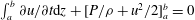 $\int _{a}^{b}\partial u/\partial t\text{d}z+[P/{\it\rho}+u^{2}/2]_{a}^{b}=0$
. Taking into account the Reynolds transport theorem produces
$\int _{a}^{b}\partial u/\partial t\text{d}z+[P/{\it\rho}+u^{2}/2]_{a}^{b}=0$
. Taking into account the Reynolds transport theorem produces
 $$\begin{eqnarray}\frac{\text{d}}{\text{d}t}\int _{a}^{b}u\text{d}z+u(a)\frac{\text{d}a}{\text{d}t}-u(b)\frac{\text{d}b}{\text{d}t}+\left[\frac{P}{{\it\rho}}+\frac{1}{2}u^{2}\right]_{a}^{b}=0.\end{eqnarray}$$
Although the exact axial velocity profile along the axis of symmetry is difficult to determine analytically, Krieg & Mohseni (Reference Krieg and Mohseni2013) recognized that the total circulation of any simply connected axisymmetric region is defined by a closed-line integral passing along the axis of symmetry (i.e.
 ${\it\Gamma}=\oint \boldsymbol{u}\boldsymbol{\cdot }\text{d}\boldsymbol{s}$
), so that this velocity integral is contained in the circulation.
${\it\Gamma}=\oint \boldsymbol{u}\boldsymbol{\cdot }\text{d}\boldsymbol{s}$
), so that this velocity integral is contained in the circulation.
To clarify the relationship between circulation and the unknown integral, first consider the semi-infinite domain on the side of the opening which extends to infinity,
 $0\leqslant z<\infty ,~0\leqslant r<\infty$
. This entire region will be referred to as the ‘jet’ for simplicity, and may contain vortex rings from multiple jetting cycles. The bounded domain on the opposite side of the opening will be referred to as the ‘cavity’. Both regions are shown in figure 1.
$0\leqslant z<\infty ,~0\leqslant r<\infty$
. This entire region will be referred to as the ‘jet’ for simplicity, and may contain vortex rings from multiple jetting cycles. The bounded domain on the opposite side of the opening will be referred to as the ‘cavity’. Both regions are shown in figure 1.
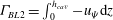
The circulation of the jet region can be written in the form
 $$\begin{eqnarray}{\it\Gamma}_{jet}=\int _{0}^{\infty }u(0,z)\text{d}z+\int _{0}^{\infty }v(r,\infty )\text{d}r+\int _{\infty }^{0}u(\infty ,z)\text{d}z+\int _{\infty }^{0}v(r,0)\text{d}r,\end{eqnarray}$$
where the closed-loop integral is broken into segments. The velocity integral along the boundaries which are at infinity (in both the axial and radial directions) can be shown to drop to zero through analysis of the stream function (Saffman Reference Saffman1992). Therefore, the velocity integral around this domain, and thus its total circulation, is the sum of the axial velocity integral along the axis of symmetry and the radial velocity integral along the orifice boundary,
 ${\it\Gamma}_{jet}=\int _{0}^{\infty }u(0,z)\text{d}z-\int _{0}^{\infty }v(r,0)\text{d}r$
.
${\it\Gamma}_{jet}=\int _{0}^{\infty }u(0,z)\text{d}z-\int _{0}^{\infty }v(r,0)\text{d}r$
.
Integrating the momentum equation from the origin to infinity (stagnation) in the axial direction, and substituting circulation and the radial velocity integral into the axial velocity integral gives the pressure at the orifice centre in terms of stagnation pressure (Krieg & Mohseni Reference Krieg and Mohseni2013):
 $$\begin{eqnarray}\frac{P_{0}}{{\it\rho}}=\frac{P_{\infty }}{{\it\rho}}-\frac{1}{2}u_{0}^{2}+\frac{\text{d}{\it\Gamma}_{jet}}{\text{d}t}+\int _{0}^{\infty }\frac{\partial v}{\partial t}\text{d}r+u_{0}\frac{\text{d}V}{\text{d}t}.\end{eqnarray}$$
Here the subscript 0 refers to any quantity at the origin,
 $r=0,z=0$
,
$r=0,z=0$
,
 $P_{\infty }$
is the stagnation pressure, and
$P_{\infty }$
is the stagnation pressure, and
 $V$
is the axial velocity of the opening/separation point, which will be non-zero if the body is moving forward or backward, or deforming in a way that moves the separation point. For the experimental testing section of this study the cavity is fixed in a stationary location, so this term will not affect these tests. It is interesting to note that a similar equation, without the separation point velocity term, was also arrived at by Krueger (Reference Krueger2005) by equating a starting jet flow to the potential field of a translating flat plate, but (2.4) is actually much more general, being valid for any unsteady vorticity distribution in the jet region.
$V$
is the axial velocity of the opening/separation point, which will be non-zero if the body is moving forward or backward, or deforming in a way that moves the separation point. For the experimental testing section of this study the cavity is fixed in a stationary location, so this term will not affect these tests. It is interesting to note that a similar equation, without the separation point velocity term, was also arrived at by Krueger (Reference Krueger2005) by equating a starting jet flow to the potential field of a translating flat plate, but (2.4) is actually much more general, being valid for any unsteady vorticity distribution in the jet region.
Next consider the control volume inside the cavity. There are several actuation methods to drive fluid motion. However, at the core of all these mechanisms is a deforming cavity boundary resulting in a change of cavity volume. In general the cavity deformation is prescribed in
 ${\it\sigma}(t)$
, and each boundary element along the length
${\it\sigma}(t)$
, and each boundary element along the length
 $l$
, has a velocity associated with the deformation, which we define as
$l$
, has a velocity associated with the deformation, which we define as
 $\boldsymbol{u}_{{\it\sigma}}(l,t)$
. At every location
$\boldsymbol{u}_{{\it\sigma}}(l,t)$
. At every location
 $l$
along the body surface we can define a local orthogonal coordinate system by
$l$
along the body surface we can define a local orthogonal coordinate system by
 $\hat{\boldsymbol{n}}$
and
$\hat{\boldsymbol{n}}$
and
 $\hat{\boldsymbol{t}}$
, which are unit vectors normal and tangential, respectively, to the surface element at that point (see figure 1). The circulation in the cavity region can likewise be broken into segments,
$\hat{\boldsymbol{t}}$
, which are unit vectors normal and tangential, respectively, to the surface element at that point (see figure 1). The circulation in the cavity region can likewise be broken into segments,
 ${\it\Gamma}_{cav}=\int _{-h}^{0}u(0,z)\text{d}z+\int _{0}^{R}v(r,0)\text{d}r+\int _{{\it\sigma}_{1}}\boldsymbol{u}_{{\it\sigma}}(l)\boldsymbol{\cdot }\hat{\boldsymbol{t}}\text{d}l$
, where
${\it\Gamma}_{cav}=\int _{-h}^{0}u(0,z)\text{d}z+\int _{0}^{R}v(r,0)\text{d}r+\int _{{\it\sigma}_{1}}\boldsymbol{u}_{{\it\sigma}}(l)\boldsymbol{\cdot }\hat{\boldsymbol{t}}\text{d}l$
, where
 $h$
is the separation between the opening and cavity surface along the axis of symmetry, and
$h$
is the separation between the opening and cavity surface along the axis of symmetry, and
 $R$
is the opening radius. Using the same analysis just performed on the jet region, we relate pressure on the surface of the cavity and at the opening and equate the line integral along the axis of symmetry to the cavity circulation:
$R$
is the opening radius. Using the same analysis just performed on the jet region, we relate pressure on the surface of the cavity and at the opening and equate the line integral along the axis of symmetry to the cavity circulation:
 $$\begin{eqnarray}\frac{P_{b}}{{\it\rho}}=\frac{P_{0}}{{\it\rho}}+\frac{1}{2}\left(u_{0}^{2}-u_{b}^{2}\right)+\frac{\text{d}{\it\Gamma}_{cav}}{\text{d}t}-\int _{0}^{R}\frac{\partial v}{\partial t}\text{d}r+\frac{\text{d}}{\text{d}t}\left(\int _{{\it\sigma}_{1}}\boldsymbol{u}_{{\it\sigma}}\boldsymbol{\cdot }\hat{\boldsymbol{t}}\text{d}l\right)-u_{0}\frac{\text{d}V}{\text{d}t}.\end{eqnarray}$$
In this equation the subscript
 $b$
refers to quantities at the intersection of the axis of symmetry and the deforming cavity boundary, and the term
$b$
refers to quantities at the intersection of the axis of symmetry and the deforming cavity boundary, and the term
 $\int _{{\it\sigma}_{1}}\boldsymbol{u}_{{\it\sigma}}\boldsymbol{\cdot }\hat{\boldsymbol{t}}\text{d}l$
is the component of circulation due to cavity deformation, which is only non-zero when the cavity boundary is stretching or collapsing. Substituting (2.4) into (2.5) allows multiple terms to cancel, and gives a relation for the pressure at the inner surface of the cavity boundary in terms of rates of change of circulation in both jet and cavity regions:
$\int _{{\it\sigma}_{1}}\boldsymbol{u}_{{\it\sigma}}\boldsymbol{\cdot }\hat{\boldsymbol{t}}\text{d}l$
is the component of circulation due to cavity deformation, which is only non-zero when the cavity boundary is stretching or collapsing. Substituting (2.4) into (2.5) allows multiple terms to cancel, and gives a relation for the pressure at the inner surface of the cavity boundary in terms of rates of change of circulation in both jet and cavity regions:
 $$\begin{eqnarray}\frac{P_{b}}{{\it\rho}}=\frac{P_{\infty }}{{\it\rho}}+\frac{\text{d}{\it\Gamma}_{jet}}{\text{d}t}+\frac{\text{d}{\it\Gamma}_{cav}}{\text{d}t}+\frac{\text{d}}{\text{d}t}\left(\int _{R}^{\infty }v\text{d}r\right)-\frac{\text{d}}{\text{d}t}\left(\int _{{\it\sigma}_{1}}\boldsymbol{u}_{{\it\sigma}}\boldsymbol{\cdot }\hat{\boldsymbol{t}}\text{d}l\right)+\frac{1}{2}u_{b}^{2}.\end{eqnarray}$$
The term
 $\text{d}/(\text{d}t)\left(\int _{R}^{\infty }v\text{d}r\right)$
can be ignored in many flows, as is the case with the experimental jet actuator, because solid boundaries extending radially outward from the opening restrict flow along that path.
$\text{d}/(\text{d}t)\left(\int _{R}^{\infty }v\text{d}r\right)$
can be ignored in many flows, as is the case with the experimental jet actuator, because solid boundaries extending radially outward from the opening restrict flow along that path.
In general there are four sources of vorticity/circulation in the deformable cavity body system which influence
 $\text{d}{\it\Gamma}_{cav}/\text{d}t$
and
$\text{d}{\it\Gamma}_{cav}/\text{d}t$
and
 $\text{d}{\it\Gamma}_{jet}/\text{d}t$
. These sources will be discussed in great detail in § 4 with the aid of experimental DPIV data. Section 4 will also lay out the functional dependence of these sources on cavity boundary position, volume flux, and the rate of change of volume flux. It should be noted here that this pressure relationship is valid during both jetting and refilling.
$\text{d}{\it\Gamma}_{jet}/\text{d}t$
. These sources will be discussed in great detail in § 4 with the aid of experimental DPIV data. Section 4 will also lay out the functional dependence of these sources on cavity boundary position, volume flux, and the rate of change of volume flux. It should be noted here that this pressure relationship is valid during both jetting and refilling.
2.2. Total jetting force
The previous subsection provides a reference pressure on the body relative to stagnation pressure. In order to determine the total instantaneous force acting on the body or the total energy output during deformation, which are the ultimate goals of this analysis, the pressure distribution over the entire body must be correlated to this reference point, which again is done by integrating the momentum equation. Here we would like to make a distinction between the different components of force acting on the body. The deformation of the cavity boundary,
 ${\it\sigma}_{1}$
, drives a transfer of fluid and vorticity between the cavity and jet regions. The total force exerted on the body due to this process will be referred to as the total jetting force,
${\it\sigma}_{1}$
, drives a transfer of fluid and vorticity between the cavity and jet regions. The total force exerted on the body due to this process will be referred to as the total jetting force,
 $F$
. The motion of the body and deformation of the outer boundary,
$F$
. The motion of the body and deformation of the outer boundary,
 ${\it\sigma}_{2}$
, also result in an altered pressure distribution, the sum of whose action we will refer to as the external hydrodynamic force. The analysis and experimental validation of this study will focus mainly on the total jetting force. Certainly the external hydrodynamic force is a rich and interesting subject, generally being lumped under external flows or boundary layer flows for rigid objects (Rosenhead Reference Rosenhead1963). The external hydrodynamic force exerts itself as a drag force for rigid bodies, but the dynamics become much more complicated for flexible bodies. In fact the external force due to vorticity cancellation on the surface of collapsing jetting bodies can greatly aid forward acceleration, as shown in Weymouth & Triantafyllou (Reference Weymouth and Triantafyllou2012, Reference Weymouth and Triantafyllou2013). But a full description and analysis of these forces is out of the scope of this work. However, much of the analysis performed on the inner cavity in determining total jetting force still applies at the outer boundary as well.
${\it\sigma}_{2}$
, also result in an altered pressure distribution, the sum of whose action we will refer to as the external hydrodynamic force. The analysis and experimental validation of this study will focus mainly on the total jetting force. Certainly the external hydrodynamic force is a rich and interesting subject, generally being lumped under external flows or boundary layer flows for rigid objects (Rosenhead Reference Rosenhead1963). The external hydrodynamic force exerts itself as a drag force for rigid bodies, but the dynamics become much more complicated for flexible bodies. In fact the external force due to vorticity cancellation on the surface of collapsing jetting bodies can greatly aid forward acceleration, as shown in Weymouth & Triantafyllou (Reference Weymouth and Triantafyllou2012, Reference Weymouth and Triantafyllou2013). But a full description and analysis of these forces is out of the scope of this work. However, much of the analysis performed on the inner cavity in determining total jetting force still applies at the outer boundary as well.
At any point along the boundary surface we can define the inviscid momentum equation in the local coordinate system providing the gradient of pressure along the surface, which would be enough to solve for the pressure distribution in the absence of viscosity. However, as was mentioned previously, stretching or collapsing of the cavity boundary contributes to the total cavity circulation. This is in the form of a boundary layer attached to the cavity surface, where obviously the inviscid momentum equation is not applicable. Fortunately, if we make the standard thin boundary approximation, the pressure gradient within the boundary layer in the normal direction is negligible,
 $\partial P/\partial \hat{\boldsymbol{n}}\approx 0$
, and the pressure on the cavity surface is equal to that just outside the boundary layer, where the inviscid momentum equation is valid. Integrating the momentum equation along the path
$\partial P/\partial \hat{\boldsymbol{n}}\approx 0$
, and the pressure on the cavity surface is equal to that just outside the boundary layer, where the inviscid momentum equation is valid. Integrating the momentum equation along the path
 ${\it\delta}$
, which is a combination of cavity and viscous layer boundaries as shown in figure 1, we determine the pressure distribution along the surface:
${\it\delta}$
, which is a combination of cavity and viscous layer boundaries as shown in figure 1, we determine the pressure distribution along the surface:
 $$\begin{eqnarray}\frac{P(l)}{{\it\rho}}=\frac{P_{b}}{{\it\rho}}-\frac{1}{2}\left(\boldsymbol{u}_{{\it\delta}}(l)\boldsymbol{\cdot }\hat{\boldsymbol{t}}\right)^{2}+\int _{l}^{l_{b}}\left(\frac{\partial \left(\boldsymbol{u}_{{\it\delta}}\boldsymbol{\cdot }\hat{\boldsymbol{t}}\right)}{\partial t}+\boldsymbol{u}_{{\it\sigma}}\boldsymbol{\cdot }\hat{\boldsymbol{n}}\frac{\partial \left(\boldsymbol{u}_{{\it\delta}}\boldsymbol{\cdot }\hat{\boldsymbol{t}}\right)}{\partial \hat{\boldsymbol{n}}}\right)\text{d}\tilde{l}.\end{eqnarray}$$
In this equation
 $P_{b}$
is the reference pressure on the cavity given in (2.6),
$P_{b}$
is the reference pressure on the cavity given in (2.6),
 $l$
is the position along the length of the curve
$l$
is the position along the length of the curve
 ${\it\sigma}_{1}$
,
${\it\sigma}_{1}$
,
 $\tilde{l}$
is a dummy variable for the length
$\tilde{l}$
is a dummy variable for the length
 $l$
,
$l$
,
 $l_{b}$
is the total length of the curve, and
$l_{b}$
is the total length of the curve, and
 $\boldsymbol{u}_{{\it\delta}}$
is the velocity along curve
$\boldsymbol{u}_{{\it\delta}}$
is the velocity along curve
 ${\it\delta}$
(
${\it\delta}$
(
 $\boldsymbol{u}_{{\it\delta}}=\boldsymbol{u}_{{\it\sigma}}$
where stretching is absent). Further, by the thin boundary layer approximation the gradient of normal velocity across the layer is small, so
$\boldsymbol{u}_{{\it\delta}}=\boldsymbol{u}_{{\it\sigma}}$
where stretching is absent). Further, by the thin boundary layer approximation the gradient of normal velocity across the layer is small, so
 $\boldsymbol{u}_{{\it\delta}}\boldsymbol{\cdot }\hat{\boldsymbol{n}}=\boldsymbol{u}_{{\it\sigma}}\boldsymbol{\cdot }\hat{\boldsymbol{n}}$
everywhere.
$\boldsymbol{u}_{{\it\delta}}\boldsymbol{\cdot }\hat{\boldsymbol{n}}=\boldsymbol{u}_{{\it\sigma}}\boldsymbol{\cdot }\hat{\boldsymbol{n}}$
everywhere.
Although this equation has several terms, the deformation of the cavity boundary is controlled to any desired motion. Therefore, the boundary velocity
 $\boldsymbol{u}_{{\it\sigma}}$
is given at the onset of the problem, and the only terms in (2.7) which are not known a priori are the tangential velocity at the edge of the boundary layer,
$\boldsymbol{u}_{{\it\sigma}}$
is given at the onset of the problem, and the only terms in (2.7) which are not known a priori are the tangential velocity at the edge of the boundary layer,
 $\boldsymbol{u}_{{\it\delta}}\boldsymbol{\cdot }\hat{\boldsymbol{t}}$
, and the normal gradient of that velocity
$\boldsymbol{u}_{{\it\delta}}\boldsymbol{\cdot }\hat{\boldsymbol{t}}$
, and the normal gradient of that velocity
 $\partial (\boldsymbol{u}_{{\it\delta}}\boldsymbol{\cdot }\hat{\boldsymbol{t}})/\partial \hat{\boldsymbol{n}}$
. In general these two terms are not easy to solve for, but the vast majority of internal flows are restricted in such a way that these terms can be simplified or approximated, as will be done for the actuator in this experiment.
$\partial (\boldsymbol{u}_{{\it\delta}}\boldsymbol{\cdot }\hat{\boldsymbol{t}})/\partial \hat{\boldsymbol{n}}$
. In general these two terms are not easy to solve for, but the vast majority of internal flows are restricted in such a way that these terms can be simplified or approximated, as will be done for the actuator in this experiment.
The pressure force on a surface element of the cavity boundary acts in the direction of the normal vector. But keep in mind that any differential surface element for an axisymmetric boundary is a circular ribbon around the axis. Therefore, any component of the pressure force pointing in the radial direction will cancel out over the entire ring and only contribute to the hoop stress in the body. For axisymmetric bodies, the total jetting force is the integral of the pressure over the cavity surface projected in the axial direction, denoted by unit vector
 $\hat{\boldsymbol{z}}$
:
$\hat{\boldsymbol{z}}$
:
 $$\begin{eqnarray}F=2{\rm\pi}\int _{{\it\sigma}_{1}}rP\hat{\boldsymbol{n}}\boldsymbol{\cdot }\hat{\boldsymbol{z}}\text{d}l.\end{eqnarray}$$
The pressure distribution on the cavity surface of a deformable jetting body has been determined with respect to system circulation dynamics and boundary deformations. Here the total jetting force was calculated from this distribution. Next we use the pressure distribution to calculate total work required to drive fluid motion,
 $W$
.
$W$
.
2.3. Total work exerted by the cavity
All interaction between the cavity and the fluid is done through pressure forces at the cavity boundaries, assuming that shear forces are small compared to pressure forces. The instantaneous power exerted at each differential surface element of this boundary is the dot product of the pressure force on the element and the instantaneous velocity of the element. Therefore, the rate at which work is being done by the cavity to generate the fluid motion is the integral of power over the entire cavity surface:
 $$\begin{eqnarray}\frac{\text{d}W}{\text{d}t}=2{\rm\pi}\int _{{\it\sigma}_{1}}rP\boldsymbol{u}_{{\it\sigma}}\boldsymbol{\cdot }\hat{\boldsymbol{n}}\text{d}l.\end{eqnarray}$$
Equations (2.8) and (2.9) provide a method to analyse the performance of deformable axisymmetric cavity bodies. If the jetting is performed for propulsion, then the useful output is the jetting force (2.8). But no matter what purpose the jetting serves, the efficiency will always be inversely proportional to total work (2.9), so given a constant output, minimizing work maximizes efficiency.
3. Experimental set-up
In order to validate the modelling of § 2, a highly adaptable jet actuator was developed to allow simultaneous measurements of total jetting force, and circulation both in and out of the cavity. The experimental set-up consists of the submerged jetting cavity connected to a PCB 1102 load cell canister, within a DPIV visualization tank. The jet actuator of this experiment is most similar to SJA devices or underwater jet thrusters, in that the outer boundary of the body as well as the cavity side walls are rigidly fixed, and cavity boundary deformation is provided by a manipulator in the back. For this experiment the cavity is constructed out of a 20 cm diameter tube with a plunger mechanism at one end and an opening to the external fluid at the other; see figure 2. The opening consists of a flat plate with a central circular orifice. The plunger is constructed out of a semi-flexible accordion bellows material, which deflects axially but maintains a constant diameter and ends in a circular flat plate. Aside from the plunger the cavity is constructed entirely from acrylic, allowing visual access and illumination of the internal flow. The plunger is driven by a linear actuator (Progressive Automation) with a potentiometer feedback mechanism to guarantee desired deflection profiles.

Figure 2. Diagram illustrating the layout of the jet actuator used in this experiment, and geometry of the problem statement.
A full jetting cycle includes both a jetting phase and a refill phase. In this investigation we aim to characterize the behaviour of the system during each phase independently as well as the effect that the phases have on each other when operating in succession. To that end the jet actuator performs both jetting and refill phases starting and ending in a resting position, as well as a full jetting cycle where the actuator draws in and immediately expels a jet of fluid. Jets which are expelled into a reservoir starting from a resting state are commonly referred to as ‘starting jets’, and to be consistent we will refer to the refill phase starting from rest as a ‘starting refill’; the full cycle cases will be referred to as a ‘pulsed jet’.
The plunger deflection program for each case can be set to any desired trajectory, but here we investigate impulsive and sinusoidal deflection programs to examine competing effects of plunger velocity and plunger acceleration (volume flux and rate of change of volume flux). The impulsive deflection program has a fast initial acceleration, after which the volume flux is held constant for the remainder of the motion, the sinusoidal program has a gradual acceleration at the start of the stroke and gradual deceleration at the end of the stroke with a higher peak velocity to maintain a consistent total volume flux with impulsive cases. The programs for the refill phase are identical to jetting, but have the opposite sign. A summary of the nozzle geometry, plunger velocity program, and starting position for each experimental trial is given in table 1. Figure 3 shows the mean deflection programs for the jetting cases, as well as the standard deviation between different trials. The sinusoidal programs are averaged for cases 1 and 2 of table 1, and cases 3 and 4 are averaged to depict the impulsive program.
Table 1. Summary of the different plunger driving conditions used in this analysis. For all cases the orifice has an inclination of
 ${\it\theta}=90^{\circ }$
and a thickness of 0.64 cm. The program refers to whether the experimental trial utilizes a sinusoidal or impulsive velocity program (see figure 3),
${\it\theta}=90^{\circ }$
and a thickness of 0.64 cm. The program refers to whether the experimental trial utilizes a sinusoidal or impulsive velocity program (see figure 3),
 $T$
is the program duration in seconds,
$T$
is the program duration in seconds,
 ${\rm\Delta}{\it\Omega}$
is the change in cavity volume,
${\rm\Delta}{\it\Omega}$
is the change in cavity volume,
 $L/D$
is a jet parameter known as the stroke ratio, and
$L/D$
is a jet parameter known as the stroke ratio, and
 $h_{0}$
is the starting value of the separation,
$h_{0}$
is the starting value of the separation,
 $h$
.
$h$
.


Figure 3. Plunger driving programs. Both plunger height and velocity are shown for (a) sinusoidal and (b) impulsive deflection programs. Error bars indicate standard deviation across all experimental cases of that type.
A plane extending through the axis of symmetry is illuminated with a laser sheet generated from a solid state 1 W Aixis 1000GamB 532 nm laser. The sheet has a thickness on the order of 1 mm. The flow is seeded with reflective neutrally buoyant particles
 ${\approx}50~{\rm\mu}\text{m}$
in diameter (manufactured by Dantec Dynamics). A data acquisition computer synchronizes the camera triggering with the plunger motion, and measures thrust signals from the load cell.
${\approx}50~{\rm\mu}\text{m}$
in diameter (manufactured by Dantec Dynamics). A data acquisition computer synchronizes the camera triggering with the plunger motion, and measures thrust signals from the load cell.
4. Circulation dynamics
In § 2 we illustrated the inherent link between cavity pressure and circulation dynamics of the cavity–jet system; now we investigate how the circulation evolves. In general there are four sources of circulation in this system, which are shown for the experimental jet actuator in figure 4. Two of these mechanisms appear in both cavity and jet regions for different phases of the jetting cycle. We call these flux and half-sink terms, respectively. The other two terms only show up inside the cavity region: one is the circulation due to cavity deformation, which is specific to cavity geometry, and the other is vortex impingement, which only occurs during the refill phase when incoming fluid impacts the cavity surface. In this section we describe each of these sources of circulation in great detail and provide modelling based on system driving parameters, which is then validated for the specific test actuator geometry. We start the discussion with vorticity flux terms, which are the largest contributor to circulation.

Figure 4. Diagram illustrating the different sources of vorticity for a cavity–jet system using vorticity fields from the experimental jet actuator as an example. Sample vorticity fields are taken from instances in cases 4 and 16 respectively. The magnitude of vorticity is shown by the colour contours. (a) Jetting phase; (b) refilling phase.
4.1. Circulation due to vorticity flux
Whether fluid is moving into the cavity or out of the cavity, as it crosses the orifice boundary there is a flux of vorticity in the direction of the moving fluid as the shear layer extends freely from the separation point into the domain with the jet.
The change in circulation of a semi-infinite domain due to flux of vorticity through a finite opening has been examined for flows with non-zero radial velocity at the opening (Rosenfeld, Katija & Dabiri Reference Rosenfeld, Katija and Dabiri2009; Krieg & Mohseni Reference Krieg and Mohseni2013), and is given by a surface integral across the opening:
 $$\begin{eqnarray}\frac{\text{d}{\it\Gamma}_{flux}}{\text{d}t}=\frac{1}{2}u\left(0,0\right)^{2}+\int _{0}^{R}\left[u\frac{\partial v}{\partial z}\right]_{z=0}\text{d}r.\end{eqnarray}$$
The accuracy of (4.1) for describing total circulation in the jet region of experimentally generated starting jets is presented for various nozzle geometries in Krieg & Mohseni (Reference Krieg and Mohseni2013). The same study also parametrized the velocity profiles at the orifice,
 $u(r,0)$
,
$u(r,0)$
,
 $v(r,0)$
and
$v(r,0)$
and
 $\partial v/\partial z(r,0)$
, for the different nozzle geometries. The effect of co-flow (which will be encountered if the cavity is internal to a moving body) on jet formation dynamics is analysed in Krueger, Dabiri & Gharib (Reference Krueger, Dabiri and Gharib2006). In addition, DPIV measurements of jet wakes behind swimming squid, where a co-flow is present, are provided by Anderson & Grosenbaugh (Reference Anderson and Grosenbaugh2005).
$\partial v/\partial z(r,0)$
, for the different nozzle geometries. The effect of co-flow (which will be encountered if the cavity is internal to a moving body) on jet formation dynamics is analysed in Krueger, Dabiri & Gharib (Reference Krueger, Dabiri and Gharib2006). In addition, DPIV measurements of jet wakes behind swimming squid, where a co-flow is present, are provided by Anderson & Grosenbaugh (Reference Anderson and Grosenbaugh2005).
The circulation in the jet region during the expulsion phase is only composed of vorticity flux terms. During the refilling phase the cavity circulation similarly grows due to vorticity flux terms, but is also affected by deformation and impingement terms which will be discussed shortly. But first we will define the other circulation source which appears in both cavity and jet regions.
4.2. Half-sink circulation
The vorticity flux term just described appears in either cavity or jet regions when the fluid is entering that region. In addition there is circulation generated in both regions when the fluid is leaving. Consider the flow in the jet region during refilling: far from the cavity the flow is roughly equivalent to that of a sink bisected in half, centred at the origin, but as we move closer to the opening the velocities remain finite. This flow can be approximated by assuming the orifice area to have a uniform sink density, with total strength equal to the volume flux entering the cavity at that time, which we will denote by
 $\dot{{\it\Omega}}$
. For the prototype actuator
$\dot{{\it\Omega}}$
. For the prototype actuator
 $\dot{{\it\Omega}}={\rm\pi}R_{p}^{2}u_{b}$
. A derivation for the circulation,
$\dot{{\it\Omega}}={\rm\pi}R_{p}^{2}u_{b}$
. A derivation for the circulation,
 ${\it\Gamma}_{HS}$
, of such a flow is provided in the appendix A by calculating the velocity of fluid passing through a set of confocal ellipsoids with constant volume flux. As shown in the appendix A, the half-sink circulation is directly proportional to the volume flux through the orifice:
${\it\Gamma}_{HS}$
, of such a flow is provided in the appendix A by calculating the velocity of fluid passing through a set of confocal ellipsoids with constant volume flux. As shown in the appendix A, the half-sink circulation is directly proportional to the volume flux through the orifice:
 $$\begin{eqnarray}{\it\Gamma}_{HS}=-C_{HS}\frac{\dot{{\it\Omega}}}{R}=-C_{HS}\frac{{\rm\pi}R_{p}^{2}u_{b}}{R}.\end{eqnarray}$$
In this equation
 $C_{HS}$
is a constant which depends on the cavity opening geometry. If the plane extending radially outward from the opening contains a solid boundary, such as flow being pushed through a circular opening in a flat plate,
$C_{HS}$
is a constant which depends on the cavity opening geometry. If the plane extending radially outward from the opening contains a solid boundary, such as flow being pushed through a circular opening in a flat plate,
 $C_{HS}=0.338$
. If the radial plane is free, like the case where flow is ingested through a tube or funnel,
$C_{HS}=0.338$
. If the radial plane is free, like the case where flow is ingested through a tube or funnel,
 $C_{HS}=0.150$
. The prototype actuator has a solid radial plane.
$C_{HS}=0.150$
. The prototype actuator has a solid radial plane.
The flow inside the cavity during jetting can also be approximated by the same half-sink flow. Figure 5 shows the measured jet circulation along with the circulation predicted by (4.2) for the jet region during refilling and the cavity region during jetting for both plunger deflection programs, cases 5, 10, 1, and 3 respectively.
 $C_{HS}$
is set to 0.338 for all cases. In this figure it can be seen that both the circulation in the jet during refilling and the circulation in the cavity during jetting are nearly identical to that of a half-sink plate.
$C_{HS}$
is set to 0.338 for all cases. In this figure it can be seen that both the circulation in the jet during refilling and the circulation in the cavity during jetting are nearly identical to that of a half-sink plate.

Figure 5. (a,b) Jet circulation,
 ${\it\Gamma}_{jet}$
, during both sinusoidal (case 5, a) and impulsive (case 10, b) refilling programs, and (c,d) cavity circulation,
${\it\Gamma}_{jet}$
, during both sinusoidal (case 5, a) and impulsive (case 10, b) refilling programs, and (c,d) cavity circulation,
 ${\it\Gamma}_{cav}$
, during both sinusoidal (case 1, c) and impulsive (case 3, d) jetting programs. For all cases actual circulation is shown by the solid line, while the dashed or dot-dashed lines show the circulation of a half-sink with strength equal to the volume flux, (4.2).
${\it\Gamma}_{cav}$
, during both sinusoidal (case 1, c) and impulsive (case 3, d) jetting programs. For all cases actual circulation is shown by the solid line, while the dashed or dot-dashed lines show the circulation of a half-sink with strength equal to the volume flux, (4.2).
Next we will describe the two sources of circulation which only occur in the finite cavity region, due to interactions with the cavity surface.
4.3. Circulation due to cavity geometry deformation
There is a circulation due to cavity geometry deformation in the direction tangent to the boundary surface which was defined in § 2,
 $\int _{{\it\sigma}_{1}}\boldsymbol{u}_{{\it\sigma}}\boldsymbol{\cdot }\hat{\boldsymbol{t}}\text{d}l$
. It should be noted here that cavity boundary deformation only contributes to total circulation if the cavity surface element moves in the direction tangent to the surface. This means that for this term to be non-zero a section of the boundary must be growing/stretching.
$\int _{{\it\sigma}_{1}}\boldsymbol{u}_{{\it\sigma}}\boldsymbol{\cdot }\hat{\boldsymbol{t}}\text{d}l$
. It should be noted here that cavity boundary deformation only contributes to total circulation if the cavity surface element moves in the direction tangent to the surface. This means that for this term to be non-zero a section of the boundary must be growing/stretching.
For this experiment the cavity boundary, which is illustrated in figure 2, only has two moving sections. The entire plunger plate moves uniformly in the axial direction, which is normal to its surface, so there is no circulation contribution. The other time-varying section of the boundary is the plunger sleeve, which extends from the plunger plate to the back of the cavity, and expands/contracts during plunger motion while maintaining a constant diameter. Due to the nature of the support structure in the plunger sleeve, the velocity varies linearly from zero at the back of the cavity to
 $u_{b}$
at the plunger plate.
$u_{b}$
at the plunger plate.
It should be noted here that from a pressure modelling standpoint, calculation of the geometry deformation circulation term is not actually necessary. This term shows up in the pressure equation (2.6). However, if the
 ${\it\Gamma}_{cav}$
term in (2.6) is split up into the different circulation sources, then the component due to boundary deformation in
${\it\Gamma}_{cav}$
term in (2.6) is split up into the different circulation sources, then the component due to boundary deformation in
 ${\it\Gamma}_{cav}$
cancels the boundary deformation term in (2.6), and the pressure at the cavity surface is a function of vorticity flux terms, vortex impingement terms, and half-sink terms. Next we look into sources of circulation due to interaction of the cavity boundary with incoming jet flow.
${\it\Gamma}_{cav}$
cancels the boundary deformation term in (2.6), and the pressure at the cavity surface is a function of vorticity flux terms, vortex impingement terms, and half-sink terms. Next we look into sources of circulation due to interaction of the cavity boundary with incoming jet flow.
4.4. Vortex ring impingement and boundary layer formation
The total cavity circulation is shown in figure 6 during a refilling cycle (case 7), as measured through DPIV along with the circulation added to the cavity region from vorticity flux across the orifice boundary. It can be seen that the total circulation is dominated by the vorticity flux term until
 ${\approx}1~\text{s}$
, when the incoming jet begins to interact with the cavity surface. The free end of the incoming shear tube spirals into a vortex ring, similar to starting jets, and as the primary ring approaches the cavity surface it grows outward, and the core area shrinks under the influence of the solid boundary and creates a boundary layer of opposite vorticity on the surface, similar to vortex rings impacting normal plane walls, which reduces the total cavity circulation.
${\approx}1~\text{s}$
, when the incoming jet begins to interact with the cavity surface. The free end of the incoming shear tube spirals into a vortex ring, similar to starting jets, and as the primary ring approaches the cavity surface it grows outward, and the core area shrinks under the influence of the solid boundary and creates a boundary layer of opposite vorticity on the surface, similar to vortex rings impacting normal plane walls, which reduces the total cavity circulation.

Figure 6. The total circulation inside the cavity during case 7 is shown with respect to time throughout the refilling process. Also shown is the integral of vorticity flux through the nozzle opening.
The formation of an opposing vorticity boundary layer clearly affects total cavity circulation, but the existence and extent of this effect varies greatly with cavity geometry. A cavity with a very large separation between the opening and the back of the cavity may never experience impingement, whereas SJAs with very shallow cavities have been observed to generate arrays of counter-rotating vortices within the cavity, especially when a crossflow is present (Utturkar et al.
Reference Utturkar, Mittal, Rampunggoon and Cattafesta2002). Unlike the previous three subsections, where the other sources of vorticity are modelled for any general cavity body, this section will focus on modelling circulation from vortex ring impingement for the particular case where the back cavity surface has a curvature which is small compared to the opening diameter, and where separation,
 $h$
, is small enough to facilitate impingement, similar to the experimental actuator.
$h$
, is small enough to facilitate impingement, similar to the experimental actuator.
The phenomenon of a vortex ring approaching a flat plate has been the subject of several studies. The first inviscid solution comes from Helmholtz (Reference Helmholtz1867), where the problem is described by two vortex rings of opposite sign sharing a common axis coming together at a planar wall. The inviscid solution accurately predicts how the vortex ring approaching the wall slows down, grows in toroidal area, and shrinks in cross-sectional area. However, very close to the wall experimental studies show a divergence from the inviscid solution because the flow near the wall induces a boundary layer of opposite vorticity affecting the trajectory (Walker et al. Reference Walker, Smith, Cerra and Doligalski1987).
Figure 7 shows the vorticity contours inside the cavity for case 7, whose circulation history is shown in figure 6, at characteristic times around the impingement marked by vertical lines in figure 6. Figure 7(a) shows the primary vortex approaching the plunger plate right before significant boundary layer growth. The development of a strong boundary layer as the leading vortex approaches the plunger surface is shown in figure 7(b,c). Finally, as the leading vortex is stretched outwards and approaches the cavity side walls another boundary layer begins to form, as is shown in figure 7(d).

Figure 7. Cavity vorticity contours at successive time steps showing boundary layer development on the surface of the plunger and cavity side wall. Positive vorticity is indicated by the dashed line contours, negative vorticity with the solid line contours, and magnitude is indicated by colour gradient. Snapshots taken from case 7, at times indicated by the vertical lines in figure 6.
Fortunately, an exact boundary layer solution is not required to determine the pressure profile, since we are only interested in the total circulation of the boundary layer and not the thickness or diffusion of that boundary layer. Therefore, the boundary layer is approximated as a shear layer on the surface of the plunger with infinitesimal thickness. The radial velocity on the plunger is zero by the no-slip condition, and the velocity just outside the shear layer can be approximated by an inviscid potential flow solution. The total boundary layer circulation is then the line integral of the inviscid velocity solution along the edge of the boundary layer. This is a valid approximation provided that the boundary layer remains attached, and is thin.
The stream function of the spiralling shear layer inside the cavity can be approximated as the sum of an equivalent, simplified, unconfined vortex structure and a series of artificial external vortices which drive the stream function to a constant value along the cavity surface boundary. The internal vortex will be equated to a single vortex ring filament, whose stream function in cylindrical coordinates (Lamb Reference Lamb1945; Saffman Reference Saffman1992) with strength
 ${\it\kappa}$
is
${\it\kappa}$
is
 $$\begin{eqnarray}\displaystyle & \displaystyle {\it\Psi}(r,z)=\frac{{\it\kappa}}{2{\rm\pi}}\left(r_{1}+r_{2}\right)\left[K({\it\lambda})-E({\it\lambda})\right]\!, & \displaystyle\end{eqnarray}$$
 $$\begin{eqnarray}\displaystyle & \displaystyle {\it\lambda}=\frac{r_{2}-r_{1}}{r_{2}+r_{1}}. & \displaystyle\end{eqnarray}$$
 ${\it\Psi}$
is the Stokes stream function,
${\it\Psi}$
is the Stokes stream function,
 $E$
and
$E$
and
 $K$
are complete elliptic integrals of the first and second kind, respectively, with modulus
$K$
are complete elliptic integrals of the first and second kind, respectively, with modulus
 ${\it\lambda}$
, and
${\it\lambda}$
, and
 $r_{1}$
and
$r_{1}$
and
 $r_{2}$
are characteristic distances defined by
$r_{2}$
are characteristic distances defined by  $$\begin{eqnarray}\left.\begin{array}{@{}l@{}}r_{2}=\left[\left(z-\bar{z}\right)^{2}+\left(r+\bar{r}\right)^{2}\right]^{1/2},\\ r_{1}=\left[\left(z-\bar{z}\right)^{2}+\left(r-\bar{r}\right)^{2}\right]^{1/2}.\end{array}\right\}\end{eqnarray}$$
The coordinate
 $[r,z]$
defines the point at which the stream function is evaluated, and the coordinate
$[r,z]$
defines the point at which the stream function is evaluated, and the coordinate
 $[\bar{r},\bar{z}]$
corresponds to the location of the vortex filament. As a first-order approximation, the strength of the vortex filament is equated to the circulation due to vorticity flux, and the location is set to the centre of vorticity in the cavity calculated from the DPIV velocity field, which will be shown to follow a predictable pattern aligning with the plunger deflection program. The centre of vorticity is calculated for each half-plane at every instant according to the integral quantities defined in Lamb (Reference Lamb1945):
$[\bar{r},\bar{z}]$
corresponds to the location of the vortex filament. As a first-order approximation, the strength of the vortex filament is equated to the circulation due to vorticity flux, and the location is set to the centre of vorticity in the cavity calculated from the DPIV velocity field, which will be shown to follow a predictable pattern aligning with the plunger deflection program. The centre of vorticity is calculated for each half-plane at every instant according to the integral quantities defined in Lamb (Reference Lamb1945):
 $$\begin{eqnarray}\bar{r}^{2}=\frac{\displaystyle \int _{A_{cav}}{\it\omega}_{-{\it\phi}}r^{2}\text{d}A}{\displaystyle \int _{A_{cav}}{\it\omega}_{-{\it\phi}}\text{d}A},\quad \bar{z}=\frac{\displaystyle \int _{A_{cav}}{\it\omega}_{-{\it\phi}}r^{2}z\text{d}A}{\displaystyle \int _{A_{cav}}{\it\omega}_{-{\it\phi}}r^{2}\text{d}A}.\end{eqnarray}$$
In this equation
 $A_{cav}$
is the cavity area bounded by the curve
$A_{cav}$
is the cavity area bounded by the curve
 ${\it\sigma}(t)$
, and
${\it\sigma}(t)$
, and
 ${\it\omega}_{-{\it\phi}}$
is identical to
${\it\omega}_{-{\it\phi}}$
is identical to
 ${\it\omega}_{{\it\phi}}$
at those locations where the sign of the vorticity is negative and equal to zero where the vorticity is positive. The radial and axial locations of the centre of vorticity calculated for sinusoidal cases 5–8 are depicted in figure 8. It can be seen that prior to interaction with the plunger, the vortex ring has a radius equal to that of the orifice, and the axial velocity is controlled by the plunger motion. The offset plunger height,
${\it\omega}_{{\it\phi}}$
at those locations where the sign of the vorticity is negative and equal to zero where the vorticity is positive. The radial and axial locations of the centre of vorticity calculated for sinusoidal cases 5–8 are depicted in figure 8. It can be seen that prior to interaction with the plunger, the vortex ring has a radius equal to that of the orifice, and the axial velocity is controlled by the plunger motion. The offset plunger height,
 $h(t)-h(0)$
, is scaled by the ratio
$h(t)-h(0)$
, is scaled by the ratio
 $R_{p}^{2}/R^{2}$
and is also included in figure 8 to show the similarity between ring and plunger trajectories. When the ring does come into contact with the plunger the toroidal radius grows in an almost linear fashion and the ring velocity decreases significantly. The trajectories of the vorticity centroid of the impulsive cases (9–12) are shown in figure 9 with similar characteristics.
$R_{p}^{2}/R^{2}$
and is also included in figure 8 to show the similarity between ring and plunger trajectories. When the ring does come into contact with the plunger the toroidal radius grows in an almost linear fashion and the ring velocity decreases significantly. The trajectories of the vorticity centroid of the impulsive cases (9–12) are shown in figure 9 with similar characteristics.

Figure 8. Radius and axial location of the centre of vorticity of the refilling jet for sinusoidal velocity programs (cases 5–8).

Figure 9. Radius and axial location of the centre of vorticity of the refilling jet for impulsive velocity programs (cases 9–12).
The stream function can be made constant along the plunger surface by adding the stream function of an opposite sign vortex ring an equal distance from the plunger surface, on the other side. Unfortunately, due to the radial asymmetry of
 $r_{1}$
and
$r_{1}$
and
 $r_{2}$
, the stream function cannot be made constant along the cavity wall by any single artificial ring. However, if the cavity side walls have a sufficiently large radius, then the effect of the wall can be approximated using the two-dimensional image vortex.
$r_{2}$
, the stream function cannot be made constant along the cavity wall by any single artificial ring. However, if the cavity side walls have a sufficiently large radius, then the effect of the wall can be approximated using the two-dimensional image vortex.

Figure 10. Total cavity circulation as determined by DPIV as well as the sum of approximated components for cases 5 (a), 8 (b), 9 (c), and 12 (d). For all figures the solid line represents the DPIV circulation data, the dot-dashed line is the total circulation from the vorticity flux, and the triangle markers are the sum of all components.
By definition the radial and axial velocities at any location are proportional to the axial and radial gradient of the stream function, respectively,
 $$\begin{eqnarray}v_{{\it\Psi}}(r,z)=-\frac{1}{r}\frac{\partial {\it\Psi}}{\partial z},\quad u_{{\it\Psi}}(r,z)=\frac{1}{r}\frac{\partial {\it\Psi}}{\partial r}.\end{eqnarray}$$
Finally the total circulation of the impingement boundary layer is calculated from this velocity field,
 ${\it\Gamma}_{BL1}=\int _{0}^{R_{p}}v_{{\it\Psi}}\text{d}r$
. Similarly there is a less significant boundary layer which forms on the inner surface of the cavity wall, which can also be calculated from the inviscid velocity field
${\it\Gamma}_{BL1}=\int _{0}^{R_{p}}v_{{\it\Psi}}\text{d}r$
. Similarly there is a less significant boundary layer which forms on the inner surface of the cavity wall, which can also be calculated from the inviscid velocity field
 ${\it\Gamma}_{BL2}=\int _{0}^{h_{cav}}-u_{{\it\Psi}}\text{d}z$
.
${\it\Gamma}_{BL2}=\int _{0}^{h_{cav}}-u_{{\it\Psi}}\text{d}z$
.
Now the total circulation in the cavity during refill can be approximated as the sum of flux, boundary deformation, and vortex ring impingement terms,
 $$\begin{eqnarray}{\it\Gamma}_{cav}=\int _{0}^{t}\left(\frac{1}{2}u_{0}^{2}+\int _{0}^{R}\left[u\frac{\partial v}{\partial z}\right]_{z=0}\text{d}r\right)\text{d}t+\frac{1}{2}u_{b}\left(h_{cav}-h\right)+{\it\Gamma}_{BL1}+{\it\Gamma}_{BL2}.\end{eqnarray}$$
Figure 10 illustrates the accuracy of this approximation for calculating the cavity circulation for starting refill cases 5, 8, 9, and 12.

Figure 11. Total cavity circulation,
 ${\it\Gamma}_{c}av$
, during sinusoidal (case 13, a) and impulsive (case 16, b) pulsed jet cycles are plotted along with cavity circulation for refilling phases with identical velocity program and starting height (cases 5, a, and 12, b, respectively). Also shown is half-sink circulation added to the refill phase starting at the moment when the pulsed jet switches from filling to jetting.
${\it\Gamma}_{c}av$
, during sinusoidal (case 13, a) and impulsive (case 16, b) pulsed jet cycles are plotted along with cavity circulation for refilling phases with identical velocity program and starting height (cases 5, a, and 12, b, respectively). Also shown is half-sink circulation added to the refill phase starting at the moment when the pulsed jet switches from filling to jetting.
It can be seen that this modelling gives a fairly accurate representation of the cavity circulation during the refill phase for the majority of the duration, but towards the end of the phase the cavity circulation continues to drop, which is not reflected in the model. This divergence from the model is due to the fact that at this time, the circulation begins to decrease because of viscous dissipation, which is not accounted for in this inviscid model. However, as will be discussed in § 5, this dissipative loss in circulation may not actually affect the pressure distribution in the same way that active generation of circulation does.
In summary, the pressure forces on the plunger are proportional to the rate of change of both jet and cavity circulation. The circulation in the jet region only involves vorticity flux and half-sink terms, whose derivatives scale with jet velocity squared and jet acceleration, respectively. The circulation in the cavity region has the same dependences but also involves boundary stretching and impingement terms, which are both functions of the specific cavity geometry and deformation programs.
4.5. Pulsed jets
For the pulsed jet cases, the cavity must be refilled prior to jet expulsion. The refilling phase generates a vortex ring within the cavity as described in the previous subsection, and in this section we look into the effect of this internal vortex ring on the circulation of the cavity and jet during the subsequent jetting cycle.
For the vast majority of cases there is actually no interaction between the internal vortex ring and the fluid exiting through the orifice, and the contribution from each can just be superposed to calculate the cavity circulation. To demonstrate this, figure 11 shows the cavity circulation for pulsed jet cases and starting refill cases with identical plunger starting height and velocity programs. At around the 2 s mark the starting refill cases terminate plunger motion, whereas the pulsed jet cases immediately initiate jetting. At this moment half-sink circulation is calculated for the pulsed jet cases according to (4.2), which is then added to the measured starting refill cavity circulation and also plotted in figure 11. It can be seen that during the jetting phase of the pulsed jet cycle the total cavity circulation matches very well with the sum of starting refill cavity circulation and half-sink circulation, verifying the lack of interaction between internal vortex ring and fluid being expelled.
5. Thrust measurements
The total jetting force is the integral of pressure forces over the surface given in (2.8) for any general cavity boundary geometry.
As was mentioned in § 3, the mechanism in the experimental jet actuator driving plunger motion is connected directly to a load cell at the top of the testing tank which measures the total instantaneous force acting on the cavity. The pressure can be integrated along the cavity boundary according to (2.7). For the test actuator geometry this is done along the plunger surface, which only has velocity components in the normal direction, so the pressure distribution is
 $$\begin{eqnarray}\frac{P(r,-h)}{{\it\rho}}=\frac{P_{b}}{{\it\rho}}-\frac{1}{2}v_{{\it\delta}}^{2}-\int _{0}^{r}\left(\frac{\partial v_{{\it\delta}}}{\partial t}+u_{b}\frac{\partial v_{{\it\delta}}}{\partial z}\right)\text{d}{\it\varpi},\end{eqnarray}$$
where
 ${\it\varpi}$
is a dummy variable for the radial coordinate
${\it\varpi}$
is a dummy variable for the radial coordinate
 $r$
, and
$r$
, and
 $v_{{\it\delta}}$
is the component of the
$v_{{\it\delta}}$
is the component of the
 ${\it\delta}$
boundary velocity,
${\it\delta}$
boundary velocity,
 $\boldsymbol{u}_{{\it\delta}}$
, in the radial direction.
$\boldsymbol{u}_{{\it\delta}}$
, in the radial direction.
 $v_{{\it\delta}}$
is zero during the jetting phase, and only has an appreciable magnitude during vortex ring impingement when a boundary layer is created on the surface of the plunger. In this instance the velocity at the edge of the boundary layer can be approximated by the potential flow solution
$v_{{\it\delta}}$
is zero during the jetting phase, and only has an appreciable magnitude during vortex ring impingement when a boundary layer is created on the surface of the plunger. In this instance the velocity at the edge of the boundary layer can be approximated by the potential flow solution
 $v_{{\it\Psi}}$
described in (4.6). By inserting (5.1) into (2.8) and reversing the order of integration, the total force on the plunger can be written as
$v_{{\it\Psi}}$
described in (4.6). By inserting (5.1) into (2.8) and reversing the order of integration, the total force on the plunger can be written as
 $$\begin{eqnarray}F_{P}={\rm\pi}R_{p}^{2}P_{b}-{\rm\pi}\int _{0}^{R_{p}}\left[v_{{\it\Psi}}^{2}+\left(R_{p}^{2}-r^{2}\right)\left(\frac{\partial v_{{\it\Psi}}}{\partial t}+u_{b}\frac{\partial v_{{\it\Psi}}}{\partial z}\right)\right]\text{d}r,\end{eqnarray}$$
which at any moment other than vortex ring impingement is simply
 $F_{p}={\rm\pi}R_{p}^{2}P_{b}$
.
$F_{p}={\rm\pi}R_{p}^{2}P_{b}$
.
There is also a decrease/increase in static pressure on the plunger surface as it is raised/lowered through the water, which corresponds to the buoyancy force. For all cases the buoyancy force is calculated from the position of the plunger at every time step and removed from the load cell thrust signal. The buoyancy force subtracted from the total force signal is modified slightly to account for the charging/discharging dynamics of the force sensor to give a more accurate representation of the dynamic pressure forces. The remaining component of the load cell thrust signal is the total jetting force, which will now be validated for the different phases of the jetting cycle.
5.1. Starting jet
The total force during the jetting phase is shown for both impulsive and sinusoidal velocity programs in figure 12. Along with the total thrust measured by the load cell, this figure shows the total jetting force calculated from (5.2). The circulation terms in (2.6) are determined from DPIV data. In this figure a positive force corresponds to compression and a negative force corresponds to tension in the load cell.

Figure 12. Comparison of total force on the cavity as measured by the load cell, with the force predicted from the DPIV circulation data, for cases 1 (a) and 3 (b).
During the jetting phase the jet circulation is entirely composed of vorticity flux terms, and the cavity circulation is just the half-sink term. As a result the thrust curve has a very similar shape to the jet velocity program. The effect of the half-sink circulation in the cavity is much more observable in the impulsive case, where the acceleration is very large at the beginning and end of the stroke, and the max velocity is relatively lower. In both cases the half-sink terms result in a negative thrust at the end of the jetting phase corresponding to cavity fluid deceleration. A similar negative thrust at the end of squid jetting is qualitatively identified by Anderson & DeMont (Reference Anderson and DeMont2000).
Changing the initial height of the plunger has no observable effect on the jetting thrust during this phase. In fact all starting jet cases tested in this study had a nearly identical total impulse averaging 0.48 N s with a standard deviation of 0.03 N s. This suggests that the parametrization of orifice velocity profiles performed by Krieg & Mohseni (Reference Krieg and Mohseni2013) can be applied during the jetting phase of any plunger configuration.
5.2. Starting refill
In figure 13 the total force measured by the load cell is plotted along with the force calculated from (5.2) for cases 5, 8, 9, and 12. At the start of the refill process there is a negative pressure force on the plunger surface opposing the plunger motion. However, as the fluid comes close to the plunger surface and begins to induce a boundary layer, a positive pressure force is generated on the plunger surface aiding the plunger motion. This phenomenon generally supports assumptions made in previous studies (Mohseni Reference Mohseni2006; Krieg & Mohseni Reference Krieg and Mohseni2008; Krieg et al. Reference Krieg, Klein, Hodgkinson and Mohseni2011) that the refill phase of pulsed jet thruster actuation has a zero net momentum transfer and zero net impulse. To further quantify this claim in table 2 we have compiled the ratio of net mechanical impulse (force integrated over time) to the integral of force magnitude over time for all refill cases investigated in this study.

Figure 13. Comparison of total jetting force as measured by the load cell, with the force predicted from (5.2) and DPIV circulation data, for cases 5 (a), 8 (b), 9 (c), and 12 (d).
Table 2. Impulse ratio: total impulse transferred during the refilling phase over the integral of force magnitude for that phase.

Similar to the jetting phase, impulsive refill programs experience a larger contribution from half-sink terms due to the large accelerations. The impingement terms also have a substantial effect, reversing the direction of thrust at the end of the cycle. Towards the end, after plunger motion has been terminated, the force predicted by (5.2) for all cases is positive due to the dissipative decrease in cavity circulation. However, the actual jetting force at these times drops to zero for all cases, demonstrating that evolution of circulation due to viscous dissipation does not affect pressure. Therefore, the inability of modelling in § 4 to capture these losses is not an issue with respect to pressure modelling.
5.3. Pulsed jet
Figure 14 shows the thrust comparison for pulsed jet cases 13, 14, 15, and 16. The total jetting force calculated by (5.2) is seen to be very accurate for all phases of the jetting cycle.

Figure 14. Comparison of total cavity force as measured by the load cell, with the force predicted from the DPIV circulation data, for cases 13 (a), 14 (b), 15 (c), and 16 (d).
6. Plunger work
The total instantaneous power which must be supplied to drive the fluid motion is given in (2.9) for any general cavity boundary deformation. The only portion of the experimental cavity boundary which moves in a direction normal to its surface is the plunger face. Moreover, since the entire plunger surface moves with a uniform velocity, the power which must be delivered by the linear actuator is the product of total jetting force and plunger velocity. The total work is then the integral of plunger power over the given cycle. This section examines both the instantaneous power and total work required for the different jetting cycles and velocity programs.
6.1. Starting jet
Figure 15 shows the plunger power required to drive the fluid motion, during sinusoidal (case 2) and impulsive (case 4) starting jet programs. The peak in plunger power for the sinusoidal program coincides with the peak in plunger velocity. The impulsive program shows a large peak at the beginning of pulsation, but this peak is actually significantly lower than the peak of the sinusoidal case. This is because the large acceleration at the beginning of the impulsive case and peak in
 $\text{d}{\it\Gamma}_{cav}/\text{d}t$
resulting in maximum plunger pressure occurs at the minimum plunger velocity, and for the remainder of pulsation the plunger is moving at a lower average velocity. The sinusoidal program is dominated by the circulation due to the flux term, which scales with
$\text{d}{\it\Gamma}_{cav}/\text{d}t$
resulting in maximum plunger pressure occurs at the minimum plunger velocity, and for the remainder of pulsation the plunger is moving at a lower average velocity. The sinusoidal program is dominated by the circulation due to the flux term, which scales with
 $u_{b}^{2}$
; the peak in pressure occurs simultaneously with the peak in velocity and plunger power scales with
$u_{b}^{2}$
; the peak in pressure occurs simultaneously with the peak in velocity and plunger power scales with
 $u_{b}^{3}$
at this point requiring relatively high power from the plunger.
$u_{b}^{3}$
at this point requiring relatively high power from the plunger.

Figure 15. Power transmitted from the plunger to the fluid during sinusoidal (case 2, a) and impulsive (case 4, b) starting jet programs. The positive shaded regions represent work being done by the plunger on the fluid, and the negative shaded regions represent work being done by the fluid on the plunger.
Furthermore, since the impulsive and sinusoidal velocity programs produce nearly identical total impulse, any difference in total work will indicate a shift in propulsive efficiency when the actuator is being used for underwater propulsion. Here we see a lower total work for the impulsive velocity program, so this will give a higher propulsive efficiency.
6.2. Starting refill
Though the net mechanical impulse of the refill phase is zero, the net work required to drive the plunger is not. Figure 16 shows the plunger power as a function of time during cases 5 and 8, and for the refill phases there is a longer period where the plunger power becomes negative. Positive power corresponds to work being done by the plunger on the fluid, and negative corresponds to work being done by the fluid on the plunger. At the beginning of refill, work must be provided by the plunger to initiate motion denoted by the green shaded region under the power curve at the beginning of motion. When the boundary layer begins to form on the plunger, signifying an ‘impact’ of the incoming fluid, the total pressure force is reversed, and at this stage of refill the fluid is actually doing work on the plunger. Unfortunately, this work cannot be recovered by the driving mechanism, so the total work required for refilling is the integral of only the positive power supplied by the plunger.

Figure 16. Power transmitted from the plunger to the fluid during sinusoidal (case 5, a) and impulsive (case 9, b) starting refill programs. The negative shaded regions correspond to work being done by the fluid on the plunger, and the positive shaded regions correspond to work being done by the plunger on the fluid.
It can be seen from figure 16 that, similar to the starting jet cases, sinusoidal programs result in a large peak power at the max velocity, whereas the impulsive case has a smaller peak at the onset of motion, and both have a period at the end where fluid is doing work on the plunger. However, the negative thrust period for the impulsive program results in very little work done on the plunger, because the negative thrust takes place late in the stroke cycle when the plunger motion is being terminated.
This shows that for both phases the work can be decreased by reducing the plunger velocity during maximum tension (i.e. driving the plunger so that the maximum pressure force and maximum plunger velocity occur out of phase). Another method to reduce the work during refilling is to reduce the magnitude of the thrust oscillation. The amplitude of thrust oscillation can be decreased by inducing impingement earlier in the refill stroke, thus reducing the total increase in circulation prior to vorticity cancellation.
The impingement boundary layer can be induced earlier quite simply by decreasing the initial separation between plunger and orifice,
 $h_{0}$
. Figure 17 shows the total work required to refill the cavity for cases 5–12, which all have equivalent volumes, orifice diameters, and refilling periods, but different programs and starting heights. It can be seen that for both sinusoidal and impulsive programs the total work is reduced by decreasing the initial plunger height. However, the sinusoidal program has a total work much larger than that of the impulsive program.
$h_{0}$
. Figure 17 shows the total work required to refill the cavity for cases 5–12, which all have equivalent volumes, orifice diameters, and refilling periods, but different programs and starting heights. It can be seen that for both sinusoidal and impulsive programs the total work is reduced by decreasing the initial plunger height. However, the sinusoidal program has a total work much larger than that of the impulsive program.

Figure 17. Total plunger work versus plunger starting height for both impulsive and sinusoidal plunger velocity programs (cases 5–12).
7. Application to biological propulsion
One of the obvious applications of this modelling is locomotory analysis of jetting marine animals. There are several marine animals which utilize cavity deformation to generate propulsion, including jellyfish, octopus, cuttlefish, and nautilus, to name a few. By far the fastest of these animals are squid, with Humboldt squid travelling an impressive 100 km in a 3–4 day period during migration (Gilly et al. Reference Gilly, Markaida, Baxter, Block, Boustany, Zeidberg, Reisenbichler, Robison, Bazzino and Salinas2006). Aside from this impressive migratory behaviour suggesting efficient swimming capabilities, recent studies (Anderson & DeMont Reference Anderson and DeMont2000; Anderson & Grosenbaugh Reference Anderson and Grosenbaugh2005; Bartol et al. Reference Bartol, Krueger, Thompson and Stewart2008, Reference Bartol, Krueger, Stewart and Thompson2009) indicate that squid may actually have propulsive efficiencies substantially higher than assumed previously. In this section we qualitatively examine squid locomotion using data from previous studies, and illustrate how the pressure and work modelling can improve upon thrust and efficiency estimations.
Some previous studies investigating jet locomotion of squids have approximated intramantle pressure according to the Bernoulli equation, assuming uniform cavity pressure, predicting pressures proportional to the jet velocity squared (Trueman Reference Trueman1968; Johnson, Soden & Trueman Reference Johnson, Soden and Trueman1972; O’Dor & Webber Reference O’Dor and Webber1986; O’Dor Reference O’Dor1988). Such a simplified pressure model has significant errors associated with the effects of vortex ring formation, nozzle geometry, boundary layer development, and fluid accelerations, which will often result in heuristic correction terms, such as the coefficient of discharge used in many of these studies. Anderson & DeMont (Reference Anderson and DeMont2000) improve upon these models while investigating the jetting of Loligo pealei by taking into account the acceleration of the fluid in the mantle cavity, and eliminating the use of the discharge coefficient. In that study an unsteady term is added involving an integration of the momentum equation internal to the cavity reminiscent of (2.2) without any terms accounting for motion of the endpoints. The additional unsteady term adds non-uniformity to the cavity pressure distribution and predicts pressure time series with features similar to those created by the half-sink terms in the present study. Here it should be noted that although the form of the unsteady term in Anderson & DeMont (Reference Anderson and DeMont2000, equation (16)) has fixed limits of spatial integration and therefore only varies in time, it is clear from the surrounding discussion that the authors meant for the term to have a sliding integration limit, thus providing spatial dependence. Subsequently Anderson & DeMont warn researchers against interpolating pressure measurement data assuming uniform cavity pressure. However, it is unclear in that study how the velocity and velocity derivative are calculated at any given location along the axis of symmetry in the cavity prior to measuring the entire flow field, and none of these models provide any means of incorporating the effects of two-dimensional jet velocity.
The circulation-based model of this paper provides a means for precisely quantifying the additional terms left out of previous pressure models. At the onset of pulsation, finite jets form a vortex ring which induces a converging radial velocity at the orifice, resulting in a higher flux rate of circulation, hydrodynamic impulse, and kinetic energy (Krieg & Mohseni Reference Krieg and Mohseni2013). This is the reason that the one-dimensional momentum approximation fails to coincide with actual impulse transfer. In the model of this paper, the increased pressure due to converging radial velocity is accounted for by the coupled increase in circulation flux
 $(\text{d}{\it\Gamma}_{jet}/\text{d}t)$
. The exact increase in circulation flux is parametrized according to nozzle geometry and jet stroke ratio by Krieg & Mohseni (Reference Krieg and Mohseni2013). The unsteady acceleration terms actually exist both inside and outside the cavity (depending on whether the animal is jetting or filling) and are quantitatively modelled in this paper in the form of the half-sink potential flow which contributes to
$(\text{d}{\it\Gamma}_{jet}/\text{d}t)$
. The exact increase in circulation flux is parametrized according to nozzle geometry and jet stroke ratio by Krieg & Mohseni (Reference Krieg and Mohseni2013). The unsteady acceleration terms actually exist both inside and outside the cavity (depending on whether the animal is jetting or filling) and are quantitatively modelled in this paper in the form of the half-sink potential flow which contributes to
 $\text{d}{\it\Gamma}_{jet}/\text{d}t$
and
$\text{d}{\it\Gamma}_{jet}/\text{d}t$
and
 $\text{d}{\it\Gamma}_{cav}/\text{d}t$
. Due to a lack of pressure measurements in Anderson & DeMont (Reference Anderson and DeMont2000), a direct quantitative comparison of pressure predicted by the circulation-based model and actual intramantle pressure could not be made.
$\text{d}{\it\Gamma}_{cav}/\text{d}t$
. Due to a lack of pressure measurements in Anderson & DeMont (Reference Anderson and DeMont2000), a direct quantitative comparison of pressure predicted by the circulation-based model and actual intramantle pressure could not be made.
Determining the propulsive efficiency of jetting animals analytically can sometimes prove to be a daunting task. As pointed out by Anderson & DeMont (Reference Anderson and DeMont2000) and Anderson & Grosenbaugh (Reference Anderson and Grosenbaugh2005), the standard Froude efficiency model is not suitable for this type of locomotion given the alternating intake and output. Furthermore, we contend that the rocket efficiency equation, as well as the similar full pulsation cycle efficiency listed in Anderson & DeMont (Reference Anderson and DeMont2000) and Anderson & Grosenbaugh (Reference Anderson and Grosenbaugh2005), may be compromised by approximating useful and total required energy assuming a steady (or average) forward velocity, and average jet velocity, when the locomotion is anything but steady. The rocket and full cycle efficiency equations are useful for identifying general trends and limits (Anderson & DeMont Reference Anderson and DeMont2000; Anderson & Grosenbaugh Reference Anderson and Grosenbaugh2005), and in some cases provide excellent agreement with measured efficiencies (Anderson & Grosenbaugh Reference Anderson and Grosenbaugh2005). But the rocket efficiency equation will not be able to distinguish between swimming cycles with equivalent average velocity and average thrust, but different jetting programs. In general the rocket efficiency equation will provide good results so long as the average jet and body velocities are similar to the higher-order means (i.e. root mean square). One of the reasons for the good agreement in Anderson & Grosenbaugh (Reference Anderson and Grosenbaugh2005) is that the L. pealei studied have a nearly impulsive jet velocity program (as will be discussed shortly) so that jet velocity and body accelerations have large periods of being nearly constant. A common observation made by those studying propulsive efficiency of marine animals is that the total work is the sum of the useful propulsive work and the wasted kinetic energy left in the wake. With the advent of DPIV measurement techniques, in studies such as Anderson & Grosenbaugh (Reference Anderson and Grosenbaugh2005), Bartol et al. (Reference Bartol, Krueger, Thompson and Stewart2008, Reference Bartol, Krueger, Stewart and Thompson2009), Moslemi & Krueger (Reference Moslemi and Krueger2009, Reference Moslemi and Krueger2011), kinetic energy in the jet wake is calculated directly from the DPIV velocity field to provide efficiency data. The only appreciable source of error with such a method is that kinetic energy measured in the wake will always be lower than the actual wasted energy, due to viscous dissipation. This error increases with decreasing Reynolds number and could become significant for small marine animals. In personal communications with Bartol & Krueger we learned that corrections were applied to reduce this source of error. An alternative methodology, for cases where the acceleration is not constant and where Reynolds number is very low, is to determine the instantaneous power transmitted to the fluid at the body surface, which can be integrated to determine the total work. Application of this technique is possible with the modelling of the present study, and does not require any more information than is used to calculate total force.
Although we cannot compare our model to pressure inside the swimming squid of Anderson & DeMont (Reference Anderson and DeMont2000), we can make qualitative observations of the jetting program. That study provides data (figures 5 and 6 in Anderson & DeMont Reference Anderson and DeMont2000, for slow and fast swimming squid respectively) for the periodic fluid volume transfer in and out of the mantle cavity, which is reproduced here for the slow swimming squid in figure 18 for convenience. It can be seen in these figures that the rate of increase or decrease in cavity volume is nearly linear during both jetting and refilling, corresponding to constant jet velocity, and a rapid acceleration when switching between the two phases. This velocity program is actually nearly identical to the impulsive velocity program used in the current study.

Figure 18. Mantle volume of L. pealei versus time during the jetting process. Figure adapted from figure 5 of Anderson & DeMont (Reference Anderson and DeMont2000), including straight lines to show the nearly linear volume flux program employed by squid.
This similarity suggests that there is, to some degree, a universal advantage to the impulsive-type velocity program. Clearly the internal mantle geometry of the squid and deformation of that cavity are vastly different from those of the test actuator here, the most obvious difference being that the mantle cavity length remains relatively constant and the volume change comes from a contraction of the mantle circumference. Despite the vastly different geometry deformations, the impulsive velocity program has probably evolved in squid swimming behaviour due to an improvement in propulsive efficiency. This suggests that the high efficiency of the impulsive velocity program, due to out-of-phase peaks in internal pressure and cavity deformation velocity, may be a universal trend for a wide variety of cavity geometry deformations.
8. Conclusion
This study derived a model for the pressure distribution inside a deformable, axisymmetric, jetting cavity body. This type of modelling is necessary in order to predict total instantaneous force acting on the cavity, which we refer to as total jetting force, as well as total energy required to drive the system. This modelling is a powerful tool in analysing such cavity–jet flows because it is based on the rate of change of total jet and cavity circulation, which in turn can be directly correlated to deformation parameters. The total instantaneous thrust of a prototype actuator was measured simultaneously with DPIV measurements allowing the total jetting force derivation to be validated for a particular geometry. The model shows good agreement with total measured thrust both during jetting and refilling of the cavity for sinusoidal and impulsive velocity programs.
It is observed in this study that the pressure distribution, and by association the jetting force and total jetting work, is a function of position, velocity, and acceleration of the deforming cavity surface. We see a decrease in total required work by reducing the separation,
 $h$
, but we also observe a dynamic interplay between velocity and acceleration of the surface, which changes with different velocity programs. The impulsive velocity program requires lower energy than the sinusoidal program because the large accelerations cause maximum force and maximum velocity to be out of phase, but the set of plunger velocity programs tested here is far from a comprehensive set of all possible plunger deflection programs. It is not hard to imagine that there might be a program which is a compromise between the two cases and a minimum is reached between the competing effects of plunger velocity and plunger acceleration. This paper lays out an analytical model for the dependence of jetting force and work on the deformation program, which is the ground work for optimization of the plunger program through variational analysis.
$h$
, but we also observe a dynamic interplay between velocity and acceleration of the surface, which changes with different velocity programs. The impulsive velocity program requires lower energy than the sinusoidal program because the large accelerations cause maximum force and maximum velocity to be out of phase, but the set of plunger velocity programs tested here is far from a comprehensive set of all possible plunger deflection programs. It is not hard to imagine that there might be a program which is a compromise between the two cases and a minimum is reached between the competing effects of plunger velocity and plunger acceleration. This paper lays out an analytical model for the dependence of jetting force and work on the deformation program, which is the ground work for optimization of the plunger program through variational analysis.
Future research will optimize both plunger height and nozzle diameter programs with respect to total impulse, total plunger work, and propulsive efficiency, for this specific actuator geometry, and will eventually optimize any general flexible cavity deformation for the same objectives. Future studies will also apply this modelling to more complicated biological cavity deformations in order to isolate locomotion-enhancing behaviours.
Acknowledgement
This work is supported by a grant from the Office of Naval Research.
Appendix A. Circulation of a finite-area uniform circular sink
As was discussed in § 4, the flow close to the opening in both cavity and jet regions, when fluid is leaving that region, can be considered equivalent to that of a circular sink plate at the nozzle orifice. By ‘sink plate’ we are referring to a circular area of velocity point-sinks. In this appendix we derive the velocity field of such a flow along with the total circulation of the region.
For a point-sink, the velocity field magnitude decreases with the distance cubed. Each distance outward defines a spherical shell with constant flux equal to the sink strength, and the velocity throughout the shell has uniform magnitude, pointing in the inward normal direction. Similar relationships can be used to derive the velocity field around a finite-area circular sink plate, if it is assumed that the flow through the plate is uniform. The sink plate can be represented by the lower bound of a family of confocal ellipsoids, all sharing a common focal ring at the nozzle radius,
 $R$
. We will model the flow by assuming each half-ellipsoid has the same volume flux as the sink plate itself,
$R$
. We will model the flow by assuming each half-ellipsoid has the same volume flux as the sink plate itself,
 $\dot{{\it\Omega}}$
. The boundary of any such ellipsoid in the axisymmetric plane is defined by the relationship
$\dot{{\it\Omega}}$
. The boundary of any such ellipsoid in the axisymmetric plane is defined by the relationship
 $$\begin{eqnarray}r=\left[\frac{\left(a^{2}-z^{2}\right)\left(R^{2}+a^{2}\right)}{a^{2}}\right]^{1/2},\end{eqnarray}$$
where each member of this family is parametrized by the semi-major axis of the ellipsoid,
 $a$
, or location of the ellipsoid on the
$a$
, or location of the ellipsoid on the
 $z$
-axis. As
$z$
-axis. As
 $a$
approaches zero, the ellipsoid approaches an infinitely thin disk at the nozzle orifice, and as
$a$
approaches zero, the ellipsoid approaches an infinitely thin disk at the nozzle orifice, and as
 $a$
approaches infinity, the ellipsoid approaches a sphere centred at the origin. Using the nozzle radius as the characteristic length scale of the problem, the positions and semi-major axis can be made dimensionless,
$a$
approaches infinity, the ellipsoid approaches a sphere centred at the origin. Using the nozzle radius as the characteristic length scale of the problem, the positions and semi-major axis can be made dimensionless,
 $r^{\star }=r/R$
,
$r^{\star }=r/R$
,
 $z^{\star }=z/R$
,
$z^{\star }=z/R$
,
 $a^{\star }=a/R$
, making a family of self-similar ellipses,
$a^{\star }=a/R$
, making a family of self-similar ellipses,
 $r^{\star }=[(a^{\star 2}-z^{\star 2})(1+a^{\star 2})/a^{\star 2}]^{1/2}$
.
$r^{\star }=[(a^{\star 2}-z^{\star 2})(1+a^{\star 2})/a^{\star 2}]^{1/2}$
.
Again the velocity is assumed to be uniform over the surface of any given ellipsoid, pointing inward, and the volume flux is constant. Therefore, the flux through any half-ellipsoid is equal to that at the nozzle orifice spread over the surface area of the half-ellipsoid. Thus the velocity at any point can be described as
 $\dot{{\it\Omega}}/S(a^{\star })$
, where
$\dot{{\it\Omega}}/S(a^{\star })$
, where
 $S$
is the surface area of the half-ellipsoid on which the point in question lies. The half-ellipsoid surface area can be calculated by revolving the ellipse equation about the
$S$
is the surface area of the half-ellipsoid on which the point in question lies. The half-ellipsoid surface area can be calculated by revolving the ellipse equation about the
 $z$
-axis:
$z$
-axis:
 $$\begin{eqnarray}S(a^{\star })={\rm\pi}R^{2}\left[\sqrt{a^{\star 2}+1}\;a^{\star 2}\text{arcsinh}\left(\frac{1}{a^{\star }}\right)+a^{\star 2}+1\right].\end{eqnarray}$$
Due to the spherical symmetry of the point-sink, any subsection of the flow cutting through the sink itself will have zero total circulation. This is not the case for the finite-area sink, which only has axial symmetry. The total circulation of a sink plate flow, bisected at the plane containing the focal ring in an unbounded domain,
 ${\it\Gamma}_{HS}$
, is
${\it\Gamma}_{HS}$
, is
 $$\begin{eqnarray}{\it\Gamma}_{HS}=\int _{0}^{\infty }u(0,z)\text{d}z+\int _{\infty }^{R}-v(r,0)\text{d}r.\end{eqnarray}$$
The velocities along the
 $r$
and
$r$
and
 $z$
axes are depicted in figure 19(a) to illustrate the asymmetry of the velocity profiles. In this figure the velocities are normalized by the velocity at the sink plate,
$z$
axes are depicted in figure 19(a) to illustrate the asymmetry of the velocity profiles. In this figure the velocities are normalized by the velocity at the sink plate,
 $\dot{{\it\Omega}}/{\rm\pi}R^{2}$
, and positions are given in normalized form. As would be expected, the two velocities converge as the distance approaches infinity, and the radial velocity is only non-zero outside the nozzle radius. The velocities shown here are for the case where the radial axis is free. For a flat-plate orifice nozzle, the velocity along the radial boundary is restricted by the no-slip condition and the total circulation is increased.
$\dot{{\it\Omega}}/{\rm\pi}R^{2}$
, and positions are given in normalized form. As would be expected, the two velocities converge as the distance approaches infinity, and the radial velocity is only non-zero outside the nozzle radius. The velocities shown here are for the case where the radial axis is free. For a flat-plate orifice nozzle, the velocity along the radial boundary is restricted by the no-slip condition and the total circulation is increased.

Figure 19. Normalized velocities along the primary axis are shown as a function of normalized position for the half-sink (a), as well as the numerically calculated circulation coefficient as a function of normalized semi-major axis (b).
Since the tangential velocities along the
 $r$
and
$r$
and
 $z$
axes are equal for an ellipsoid of a given semi-major axis, it makes sense to use this parameter as the integration variable for the circulation, taking into account spatial scaling along each axis,
$z$
axes are equal for an ellipsoid of a given semi-major axis, it makes sense to use this parameter as the integration variable for the circulation, taking into account spatial scaling along each axis,
 $[\text{d}z^{\star }/\text{d}a^{\star }]_{r^{\star }=0}=1$
and
$[\text{d}z^{\star }/\text{d}a^{\star }]_{r^{\star }=0}=1$
and
 $[\text{d}r^{\star }/\text{d}a^{\star }]_{z^{\star }=0}=a^{\star }/\sqrt{1+a^{\star 2}}$
respectively. By such an approach the total circulation for both free and bounded conditions can be determined by a single integral quantity:
$[\text{d}r^{\star }/\text{d}a^{\star }]_{z^{\star }=0}=a^{\star }/\sqrt{1+a^{\star 2}}$
respectively. By such an approach the total circulation for both free and bounded conditions can be determined by a single integral quantity:
 $$\begin{eqnarray}{\it\Gamma}_{HS}=\int _{0}^{\infty }\frac{\dot{{\it\Omega}}}{S(a^{\star })}R(B-1)\text{d}a^{\star },\quad B=\left\{\begin{array}{@{}ll@{}}\displaystyle \frac{a}{\sqrt{1+a^{2}}},\quad & \text{free boundary},\\ 0,\quad & \text{restricted boundary},\end{array}\right.\end{eqnarray}$$
where
 $S(a^{\star })$
is defined in (A 2). By moving the parameters
$S(a^{\star })$
is defined in (A 2). By moving the parameters
 $\dot{{\it\Omega}}$
and
$\dot{{\it\Omega}}$
and
 $R$
out of the integral, since they only depend on time, the remaining integrand is purely a function of
$R$
out of the integral, since they only depend on time, the remaining integrand is purely a function of
 $a^{\star }$
and the integral quantity is some constant, leading to a drastically simplified circulation equation:
$a^{\star }$
and the integral quantity is some constant, leading to a drastically simplified circulation equation:
 $$\begin{eqnarray}{\it\Gamma}_{HS}=-C_{HS}\frac{\dot{{\it\Omega}}}{R}.\end{eqnarray}$$
The integral quantity represented by
 $C_{HS}$
cannot be simplified in terms of elementary functions. Therefore we numerically integrated equation (A 4) for a range of upper limits of integration to demonstrate convergence. The value of
$C_{HS}$
cannot be simplified in terms of elementary functions. Therefore we numerically integrated equation (A 4) for a range of upper limits of integration to demonstrate convergence. The value of
 $C_{HS}$
as the upper limit approaches infinity is shown for both radial boundary conditions in figure 19(b). It can be seen in this figure that within a very short distance the circulation begins to converge upon a finite value due to the exponentially decreasing velocity. To within the first 3 digits the circulation coefficient is equal to
$C_{HS}$
as the upper limit approaches infinity is shown for both radial boundary conditions in figure 19(b). It can be seen in this figure that within a very short distance the circulation begins to converge upon a finite value due to the exponentially decreasing velocity. To within the first 3 digits the circulation coefficient is equal to
 $C_{HS}=0.338$
for the restricted radial boundary condition and
$C_{HS}=0.338$
for the restricted radial boundary condition and
 $C_{HS}=0.150$
for the free radial boundary condition.
$C_{HS}=0.150$
for the free radial boundary condition.


