


INTRODUCTION
Traditionally, conservation strategies have relied on the intrinsic value that people place on nature to generate support for protecting biodiversity and thereby restrain current global species loss (Butchart et al. Reference Butchart, Walpole, Collen, van Strien, Scharlemann, Almond, Baillie, Bomhard, Brown and Bruno2010). Biodiversity conservation projects face many challenges, including limited funding, social and political support, as well as pressure to sustain economic development, which together can hinder implementation. More recently, the supply of ecosystem services (ES) has also been recognized as increasingly precarious. Since ES are so important for human well-being, there has been increasing interest in ensuring their sustainability, notably through land protection and related conservation actions (MA [Millennium Ecosystem Assessment] 2005; Margules & Sarkar Reference Margules and Sarkar2007). Yet, some conservationists have expressed concerns that protecting ES may distract conservation efforts from a broader focus on protecting all biodiversity, and tend to neglect or exclude species that provide no ES (McCauley Reference McCauley2006; Redford & Adams Reference Redford and Adams2009; Deliège & Neuteleers Reference Deliège and Neuteleers2014). However, the potential of ES to promote the social acceptance of implementing conservation projects and their potential to promote the political and economic support of these projects has also been identified (Goldman et al. Reference Goldman, Tallis, Kareiva and Daily2008; Reyers et al. Reference Reyers, Polasky, Tallis, Mooney and Larigauderie2012; Cimon-Morin et al. Reference Cimon-Morin, Darveau and Poulin2014a ). ES could thus enable the use of supplementary strategies for protecting biodiversity (Reyers et al. Reference Reyers, Polasky, Tallis, Mooney and Larigauderie2012; Cimon-Morin et al. Reference Cimon-Morin, Darveau and Poulin2014a ) if the conservation of both can be aligned through overlapping actions.
While all ES imply some level of biodiversity, the exact nature of their relationship is not easily determined (Mace et al. Reference Mace, Norris and Fitter2012; Reyers et al. Reference Reyers, Polasky, Tallis, Mooney and Larigauderie2012; Harrison et al. Reference Harrison, Berry, Simpson, Haslett, Blicharska, Bucur, Dunford, Egoh, Garcia-Llorente, Geamănă, Geertsema, Lommelen, Meiresonne and Turkelboom2014). Joint conservation actions are only possible if (1) areas prioritized for biodiversity and ES are spatially congruent (for example if biodiversity represents ES provision), or (2) a complementary set of sites can be identified. However, a growing number of studies have found low to moderate spatial concordance between priority areas for ES and biodiversity in conservation assessments (reviewed in Cimon-Morin et al. Reference Cimon-Morin, Darveau and Poulin2013). To ensure more efficient conservation solutions, it has been suggested that systematic conservation planning procedures focus on both objectives through site complementarity rather than on congruence (Thomas et al. Reference Thomas, Anderson, Moilanen, Eigenbrod, Heinemeyer, Quaife, Roy, Gillings, Armsworth and Gaston2012; Cimon-Morin et al. Reference Cimon-Morin, Darveau and Poulin2013). Complementarity implies that conservation areas can be linked synergistically by their inherent features to achieve conservation objectives efficiently (Kukkala & Moilanen Reference Kukkala and Moilanen2013). This may be a way to identify priority areas and promote the conservation of localized biodiversity features even if they occur in environments that provide few ES, and vice versa.
Remote regions, such as the Canadian boreal zone (Brandt Reference Brandt2009), contain some of the world's last remnants of wilderness and still harbour near-pristine ecosystems. Not only do they represent unique opportunities for biodiversity conservation (Schindler & Lee Reference Schindler and Lee2010; Berteaux Reference Berteaux2013; McCauley et al. Reference McCauley, Power, Bird, McInturff, Dunbar, Durham, Micheli and Young2013), these regions also provide important local to global flow scale ES to human populations (Kareiva & Marvier Reference Kareiva and Marvier2003; Schindler & Lee Reference Schindler and Lee2010; McCauley et al. Reference McCauley, Power, Bird, McInturff, Dunbar, Durham, Micheli and Young2013). People living in remote regions generally have a more utilitarian view of nature and its conservation (Berteaux Reference Berteaux2013; Failing et al. Reference Failing, Gregory and Higgins2013) than those living in urban centres or biodiversity conservationists. Preserving a vast range of provisioning and cultural services can be particularly important in remote regions, where inhabitants generally draw a higher portion of their necessities of life from their surrounding ecosystems than do urban dwellers. Some populations, often indigenous communities, even directly depend, at least seasonally, on the resources they can obtain from ecosystems (Foote & Krogman Reference Foote and Krogman2006). Often considered self-protected simply due to their remoteness, these regions have generally not benefited from conservation efforts, especially in regard to protecting ES. While some conservationists argue that conservation efforts should focus on densely-populated regions where rates of biodiversity losses are higher (Craigie et al. Reference Craigie, Pressey and Barnes2014), the scarcity of natural resources in the vicinity of densely populated areas, human population expansion, new technologies and extension of transportation networks have all increased interest in developing outlying regions (Foote & Krogman Reference Foote and Krogman2006; Kramer et al. Reference Kramer, Urquhart and Schmitt2009; Berteaux Reference Berteaux2013). Consequently, there are great opportunities for sound planning before development in remote regions, and intervention to secure and manage both ES supply and biodiversity in these areas is long overdue (Kareiva & Marvier Reference Kareiva and Marvier2003; McCauley et al. Reference McCauley, Power, Bird, McInturff, Dunbar, Durham, Micheli and Young2013, Reference McCauley, Young, Power, Bird, Durham, McInturff, Dunbar and Micheli2014).
In contrast to strategies for biodiversity conservation, setting aside areas for safeguarding ES that are located at a distance from human beneficiaries may be irrelevant for most ES (Reyers et al. Reference Reyers, Polasky, Tallis, Mooney and Larigauderie2012; Cimon-Morin et al. Reference Cimon-Morin, Darveau and Poulin2013, Reference Cimon-Morin, Darveau and Poulin2015). Indeed, most ES do not provide benefits everywhere they are biophysically supplied, for example, due to lack of physical access or demand (Tallis et al. Reference Tallis, Polasky, Lozano and Wolny2012). This is particularly true for local flow scale ES (such as provisioning and most cultural services), whose benefits must be obtained at or near the location where their supply is safeguarded. To be effective, ES conservation must focus on actual-use supply, defined as accessible supply and demand occurring simultaneously at the same site (see Cimon-Morin et al. Reference Cimon-Morin, Darveau and Poulin2014b ). In a previous study, we found that identifying priority areas based on ES supply alone assembled conservation networks up to five times less in demand and with great spatial discrepancies when compared with approaches targeting the actual-use supply; this also resulted in the selection of some sites inaccessible to beneficiaries (Cimon-Morin et al. Reference Cimon-Morin, Darveau and Poulin2014b ). However, these novel approaches may introduce a spatial bias toward sites in proximity to human settlements, which could further undermine the already weak congruence between priority areas for ES and those for biodiversity.
Considering the sparse distribution of human populations in remote regions, it is still unclear whether biodiversity and actual-use supply of ES could overlap sufficiently to enable the development of conservation strategies that would safeguard both simultaneously. To evaluate the complementarity between biodiversity and ES, we conducted a case study of systematic conservation planning in a remote, sparsely-populated region of eastern Canada, focusing on biodiversity and ten ES associated with freshwater wetlands. Wetland conservation is of particular interest because these ecosystems are rich in biodiversity, while also being generous providers of important ES (Foote & Krogman Reference Foote and Krogman2006; Schindler & Lee Reference Schindler and Lee2010). We first investigated the spatial congruence between ES and biodiversity during conservation assessment by looking at the amount of each ES captured incidentally by a conservation plan that targeted wetland biodiversity and vice versa. We then compared these conservation plans with two other conservation scenarios that considered both biodiversity and ES features simultaneously. Finally, we considered strategies for aligning ES and biodiversity conservation under such circumstances to preserve both most effectively.
METHODS
Study area
The study was undertaken in an area extending across the Lower North Shore Plateau ecoregion and into the southern portion of the Central Labrador ecoregion in boreal Quebec (Fig. 1; Li & Ducruc Reference Li and Ducruc1999), which corresponds to the eastern half of the continental part of the Central Laurentians and Mecatina Plateau ecoregion level III of North America (Wiken et al. Reference Wiken, Jiménez Nava and Griffith2011). It covers 137 565 km2 and encompasses approximately 12 350 inhabitants (0.09 inhabitants km−2), of whom 9800 are dispersed across fifteen municipalities and 2550 are distributed in four First Nations communities (Gouvernement du Québec 2013). The study area is currently minimally developed, and the main economic activities are mining, hydroelectric energy production, aluminium processing and commercial fishing in the gulf of the Saint Lawrence River (CRÉ [Conférence régionale des élus de la Côte-Nord] 2010). Forestry accounts for a small part of the local economy, because the study area is located at the northern limit of the commercial boreal forest; only 10% of the study area is covered by productive commercial stands (MRNF [ministère des Ressources naturelles et de la Faune du Québec] 2012). The minimal mapping unit of the Natural Capital Inventory dataset (Ducruc Reference Ducruc1985), originally compiled for ecological classification of the territory, was used to divide the study area into 16 026 planning units. The planning units are of irregular shape and size (mean of 8.5 ± 15 km2) because they are delimited by significant and permanent environmental features, such as landscape topography, surface deposits and water bodies. All mapping was performed using ArcGIS 10.0 (ESRI [Environmental Systems Research Institute] 2012).
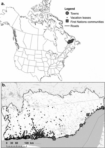
Figure 1 (a) Location of the study area, (b) indicating roads and major towns, First Nations communities and vacation leases on Crown lands.
Wetland biodiversity surrogates
Data on species distribution are scarce for the study area, and cannot easily be collected given time and budget constraints. To rely on the most complete data available, we used a combination of three wetland biodiversity surrogates to represent the study area's wetland biodiversity (Margules & Sarkar Reference Margules and Sarkar2007). First, we mapped 16 wetland types. We then assessed the composition and richness of wetland types at the scale of the planning unit to generate two wetland assemblage surrogates. Traditionally, assemblages represent different combinations of items, such as species, community or habitat type, as well as the interactions between them, and therefore reflect greater ecological complexity than individual taxa (Margules & Sarkar Reference Margules and Sarkar2007). Wetland composition classes were obtained using a clustering procedure that aggregated planning units according to the similarity of their wetland composition; wetland richness classes were based on the number of wetland types within each planning unit.
Wetland types
We mapped 16 wetland and aquatic habitat types, the largest number possible using the most complete data available. We used the Natural Capital Inventory dataset (Ducruc Reference Ducruc1985), which contains aggregated information on descriptive variables at the planning unit scale, such as surface deposit (for example, organic or mineral), drainage and vegetation cover, to infer the relative coverage proportion of one mineral wetland type (including both marshes and swamps) and 10 peatland types. More specifically, we differentiated four types of ombrotrophic peatlands (bogs) based on the presence of ombrotrophic organic deposits, peat depth (thick or thin; threshold of ± 1 m) and vegetation cover (forested or not). We also distinguished between six minerotrophic peatland types (fens) among the minerotrophic organic deposits using peat depth (thick or thin; threshold of ± 1 m) and vegetation cover (forested or not; presence/absence of patterns or strings). Five aquatic habitats (streams, rivers, ponds, shallow zones of lakes, deep zones of lakes; Ménard et al. Reference Ménard, Darveau and Imbeau2013) were extracted from the CanVec v8.0 dataset (NRC [Natural Resources Canada] 2011). We used a 100 m distance buffer from the shoreline to discriminate between shallow zones of lakes (littoral zones, < 2 m deep) and deep-water zones (Lemelin & Darveau Reference Lemelin and Darveau2008). This distinction was based on the premise that these two types of habitats differ in their capacity to generate ES supply, notably for waterfowl-related ES (Lemelin et al. Reference Lemelin, Darveau, Imbeau and Bordage2010). While streams, rivers, ponds, and shallow zones of lakes are part of the shallow water class (> 2 m deep) of the Canadian wetlands classification system (NWWG [National Wetlands Working Group] 1997), we also decided to consider deep-water zones of lakes in our conservation assessments (hereafter included in ‘wetland type features’). This decision was made to facilitate management and conservation decisions, since shallow and deep-water zones are directly associated, and the boundary between them may fluctuate over time (at least seasonally; Cowardin & Golet Reference Cowardin and Golet1995). The total relative coverage of the five aquatic habitats was calculated for each planning unit. The area covered by linear vector features, such as streams and rivers, was estimated by generating a raster grid with a 25-m pixel resolution. Ten per cent of the study area is covered by wetlands and another 17% by aquatic habitats.
Wetland composition classes
A wetland composition class represents a set of planning units that are similar in terms of frequency and abundance of wetland types. The cascade KM function from the VEGAN package (Borcard et al. Reference Borcard, Gillet and Legendre2011; Legendre & Legendre Reference Legendre and Legendre2012) of R version 3.0.1 software (R Development Core Team 2013) was used to identify the optimal number of different classes based on our data. The function proposed 11 composition classes. Then, the K-means portioning analysis in R (Borcard et al. Reference Borcard, Gillet and Legendre2011; Legendre & Legendre Reference Legendre and Legendre2012), a non-hierarchical clustering method, was used to associate each planning unit to one of the 11 wetland composition classes.
Wetland richness classes
Wetland richness class was measured as the number of each wetland type per planning unit. Wetland richness classes ranged from 0 to 13, as no unit had the full array of 16 wetland types.
Ecosystem services
Ecosystem services selection
Based on the availability of spatial data, we selected ten wetland ES (five provisioning, three cultural and two regulating services) of global significance or for which the sustainability of supply is important, notably with regard to the livelihood of local communities and tourism-related activities. Provisioning services included (1) moose and (2) waterfowl hunting, (3) salmon and (4) trout angling, and (5) cloudberry picking. Although, game species uptake is often considered as a cultural service, we chose to classify it a provisioning service because, in the context of our study, these ES are more often used as a primary food source. For example, a recent survey revealed that among the non-aboriginal inhabitants of our study area, 27% practise moose hunting, 15% waterfowl hunting, 51% trout angling and 53% wild berry picking (Bergeron Reference Bergeron2014). Among those surveyed, 74% had consumed moose meat, 80% trout and 71% berries originating from the study area at least once in the last year. The cultural services included (6) aesthetics, (7) cultural sites used by First Nations for subsistence uptake, and (8) the existence value of woodland caribou (an iconic species in Canada). First Nations subsistence uptake, including traditional hunting, fishing and fruit picking practised by these communities, was considered apart from the other services since it does not involve the same beneficiaries who, among others, have greater access to the territory (namely lower dependence on roads than non-First Nations inhabitants). Regulating services included (9) flood control and (10) carbon storage. These ten services are compatible with conservation actions because they could be safeguarded at least under one of the protected area categories of the International Union for Conservation of Nature (IUCN; Dudley Reference Dudley2008). Even our provisioning services can be included in conservation, since restrictions on practices (low land-use intensity; for example subsistence uptake versus commercial uptake) ensure sustainability and preclude biodiversity loss (Cimon-Morin et al. Reference Cimon-Morin, Darveau and Poulin2013).
Mapping the biophysical supply and potential-use supply of ecosystem services
ES supply was first mapped according to the biophysical capacity of wetland types to provide an ES in each planning unit (namely biophysical supply, see Supplementary material for a description of and data on how each ES was mapped). However, mapping ES biophysical supply alone does not provide sufficient data for making appropriate conservation choices because ES do not necessarily provide benefits to human populations everywhere they are produced (Cimon-Morin et al. Reference Cimon-Morin, Darveau and Poulin2014b , Reference Cimon-Morin, Darveau and Poulin2015). Therefore, ES were mapped with regard to potential-use supply (PUS), which is a subset of the biophysical supply that is accessible to beneficiaries. In other words, we associated each ES with the spatial flow scale at which it delivers benefits to beneficiaries (local, regional or global) and we used proxies of human occupancy (for example, roads, vacation leases on Crown lands, outfitters, or towns) to identify the set of planning units that deliver accessible benefits to humans. Seven of our ES have a local flow scale: moose and waterfowl hunting, salmon and trout angling, cloudberry picking, aesthetics, and cultural sites used by First Nations for subsistence uptake. Applied to a conservation context, a local spatial flow scale means that beneficiaries must approach or enter the protected area where the ES is supplied to obtain its benefits (hereafter referred as ‘local flow ES’). One ES, flood control, has a regional flow, and the final two, the existence value of woodland caribou and carbon storage, have more global importance.
More specifically, to identify the spatial range of ES potential-use supply, the following proxies of accessibility and of human occupancy were used for local flow ES (for cultural ES sites, see Supplementary material): (1) a 1 km buffer zone around all types of roads and human settlements, such as leases of vacation lots on public lands (mostly used for fishing- and hunting-related activities), and (2) the area occupied by outfitters offering the targeted ES. While these proxies may be a conservative estimate of planning unit accessibility, we believe that the majority of human uses for the targeted local flow ES will take place within these limits. Therefore, planning units that fall outside the spatial range of benefit delivery for an individual ES were considered to provide no accessible (or direct-use) benefits and were not considered for the conservation of this ES’ supply (in other words, the planning unit feature value was set to nil). For the sole regional flow scale ES, that is, flood control, only the planning units present in watersheds containing human infrastructures were retained in the PUS. For the two global flow ES, the BS and the PUS were identical.
Mapping demand for ecosystem services
At the planning region scale, assessing an ES demand quantitatively can provide information on the quantity of accessible supply that needs to be safeguarded (namely setting conservation targets). This can ensure that beneficiaries’ needs are met, while preventing the expenditure of unnecessary conservation resources on safeguarding a surplus of ES supply. Demand within the planning region (hereafter referred to as simply ‘demand’) can also be assessed at a finer scale in terms of the probability that a specific location be used or needed for the accessible provision of a particular service to a given set of beneficiaries. Quantitatively assessing the demand for ES in each planning unit is particularly useful to discriminate among and to prioritize sites providing accessible benefits to beneficiaries because (1) accessible benefits are not necessarily in demand and (2) sites with the highest supply are not necessarily those that are the most important in fulfilling beneficiary demand (Cimon-Morin et al. Reference Cimon-Morin, Darveau and Poulin2014b , Reference Cimon-Morin, Darveau and Poulin2015).
Accordingly, we mapped ES demand for each ES (see Supplementary material for a description of and data on how demand for each ES was mapped, and specifically Fig. S2 for the spatial range of each ES demand). Demand for global flow ES was considered equal across their PUS range. For regional flow ES (namely flood control), the demand may vary according to human population density and the presence of human infrastructures (such as roads or bridges). However, we were not able to establish precise demand values for each watershed. For the purpose of this study, we assumed that demand for regional flow ES is also equal across the spatial range of their PUS. Demand for most local flow scale ES often involves the movement of their beneficiaries, who must go to where the ES is supplied in order to benefit from it. For moose hunting and salmon angling, primary data about demand was available. Demand for the other local flow ES was modelled using proxies of human usage, such as (1) a 30 km buffer zone to the nearest towns, (2) a 1 km buffer zone to vacation leases, and (3) the area occupied by outfitters. The 30 km distance from towns was preferred over a distance decay function because, in this remote region, people have good knowledge of the land and tend to repeatedly use specific spots for an ES. These proxies, as well as those used to map the PUS, are context-specific and were weighted for each ES specifically by previous social assessments and expert knowledge of human use of the territory (such as quantity of possible users and the permanency of use; Hydro-Québec 2007). For example, outfitters and vacation leases are strong predictors of demand for angling but are less predictive of wild fruit picking. Thus, a planning unit containing an outfitter and vacation leases will have a greater demand score for angling than a planning unit that does not contain these features.
The actual-use supply of ecosystem services
We defined the actual-use supply of an ES as accessible supply and demand occurring simultaneously at the same site. Safeguarding actual-use supply of an ES, notably by targeting directly in site selection procedures the potential-use supply and demand, allows for more efficient ES conservation choices (see Cimon-Morin et al. Reference Cimon-Morin, Darveau and Poulin2014b , Reference Cimon-Morin, Darveau and Poulin2015). For example, setting adequate conservation targets for moose potential-use supply should ensure the conservation of moose populations and habitats, while demand will ensure that moose are protected where they are also hunted by beneficiaries (Cimon-Morin et al. Reference Cimon-Morin, Darveau and Poulin2015). Experts were consulted for both quantitative assessment and validation of supply and demand mapping for each ES.
Conservation software and scenarios
Conservation planning software
Systematic conservation planning (SCP), a multi-step operational approach to planning and prioritizing areas for conservation (Margules & Sarkar Reference Margules and Sarkar2007), was developed to increase conservation efficiency. We assembled conservation networks using C-Plan v4.0 conservation planning software (Pressey et al. Reference Pressey, Watts, Barrett, Ridges, Moilanen, Wilson and Possingham2009). C-Plan algorithm selects sites primarily based on their irreplaceability measures, that is to say, the likelihood that a given site will need to be selected for the efficient achievement of conservation objectives (Kukkala & Moilanen Reference Kukkala and Moilanen2013). Calculating irreplaceability generally implicitly integrates complementarity (Kukkala & Moilanen Reference Kukkala and Moilanen2013). We used the area of planning units as a proxy for budget constraint in order to identify the minimum set of sites that attain conservation targets for all features while minimizing the total selected area (namely budget).
The biodiversity scenario (or BD)
The extent of wetlands that need to be protected to ensure their persistence is not well documented. Therefore, we chose to assemble conservation networks to protect six samples of 1%, 5%, 10%, 15%, 20% and 25% of all our wetland biodiversity surrogates (see above). Within these samples, we used the coarse-filter approach to set quantitative targets for each particular wetland biodiversity feature. The coarse filter implies that the conservation of a representative sample of all ecosystem types and natural communities inventoried should ‘ensure representation’ (of the constituents of a particular ecological level) and provide habitats for the majority of species in the region, even up to 90% under some circumstances (Noss Reference Noss1987; Lemelin & Darveau Reference Lemelin and Darveau2006; Hunter & Schmiegelow Reference Hunter and Schmiegelow2011). In data-scarce regions such as our study area, the coarse filter is generally applied at the ecoregion scale (c. 100 000 km2; Lemelin & Darveau Reference Lemelin and Darveau2006). Representative targets for wetland types were based on their total area, while targets for wetland composition classes and richness classes were based on their total number of occurrences. It took approximately 1%, 6%, 10%, 14%, 19% and 24% of the study area to achieve the six samples of wetland biodiversity features, respectively. These area thresholds were then used as budget limitations in the other conservation scenarios (see below) to establish networks of similar total area.
The null scenario (or null)
Planning units were randomly selected until budget limitation thresholds were attained. We used 1%, 6%, 10%, 14%, 19% and 24% of the study area as budget limitations to assemble the six networks.
The ecosystem services actual-use supply (or AUS)
Setting quantitative conservation targets for ES features is a difficult task (Egoh et al. Reference Egoh, Reyers, Rouget and Richardson2011). Consequently, instead of setting arbitrary targets, we chose to use the optimal amount of the ten ES that can be secured given fixed budget (area) thresholds. The budget thresholds used were the same as the total area required to achieve all targets in the biodiversity scenario above. Accordingly, we used 1%, 6%, 10%, 14%, 19% and 24% of the study area as budget limitations to assemble the six networks. This scenario considered ES potential-use supply and demand in site selection, which together enable the selection of ES actual-use supply (Cimon-Morin et al. Reference Cimon-Morin, Darveau and Poulin2014b , Reference Cimon-Morin, Darveau and Poulin2015). Conservation targets for the scenario seeking both ES and a representative sample of biodiversity, as described below (see the following section) were set based on the assessment of how much ES potential-use supply and demand was safeguarded under each area threshold.
The ecosystem services actual-use supply and biodiversity scenario (or AUS-BD)
Given a maximum total budget, this scenario considers ES potential-use supply, local flow ES demand and biodiversity features simultaneously. Targets for wetland biodiversity features were the same as for the biodiversity scenario, while targets for ES potential-use supply and demand were based on the optimal amount of each ES feature secured by the AUS scenario under each area threshold. We used 1%, 6%, 10%, 14%, 19% and 24% of the study area as budget limitations to assemble six networks. Once the network reached the total allowed budget, the selection process ended, despite not reaching targets for all conservation features.
The AUS-BD unconstrained scenario (or AUS-BD unconstrained)
This scenario is similar to the AUS-BD scenario, with the sole distinction that no budget limitations were used. Each ES potential-use supply, ES demand and biodiversity feature was therefore allowed to reach its assigned target.
Conservation network analysis
Conservation networks were compared based on the fraction of features that reached or exceeded their targets, and based on the utility value of targeted features. The utility value is the mean level of representation of targeted features and was therefore measured as the mean level of deviation from targets. A feature was considered to be underrepresented when it did not reach the expected thresholds (targets) and a feature was categorized as overrepresented when it exceeded the targets. Finally, considering the planning unit area as a proxy for cost may incorrectly lead to the assumption that cost is homogenous across the study area; areas with high levels of natural resources (such as mineral deposits and commercial stands) and demand (closer to human populations) are likely to be more expensive than other areas. However, while the use of actual cost data may have changed the spatial configuration of the conservation networks, it would not have changed the interpretation of the results.
RESULTS
Planning for biodiversity or ES alone
By quantifying the biodiversity and ES features captured incidentally by the scenarios based on either biodiversity (BD) or ES actual-use supply (AUS), we were able to determine to what extent ES and biodiversity could represent each other during conservation planning in the context of sparsely populated areas. These scenarios resulted in spatially distinct networks (Fig. S3, see Supplementary material). While the sites selected by the biodiversity scenario were widely distributed across the study area, the AUS scenario resulted in an expected clustering of the selected sites near human populations (Fig. 1; Fig. S3, see Supplementary material).
Biodiversity conservation planning that did not explicitly include ES resulted in reserve networks that incidentally safeguarded a low level of ES supply and demand (Fig. 2 a, b) Notably, local flow ES potential-use supply was on average underrepresented by 57%. Similarly, by excluding demand for cultural sites that exceeded target thresholds by 225%, demand for the other local flow ES was underrepresented by 61% (see Table 1 for individual values).
Table 1 Mean deviation (%) from targets for indivudual ecosystem service features under the five conservation scenarios tested. A negative value indicates that the target was not met, a zero value indicates that the target was met, while a positive value indicates that the target was exceeded. Mean values were calculated based on the results of six networks for each conservation scenario. Potential-use supply of ecosystem services refers to the supply that is accessible to beneficiaries and is a fraction of their total biophysical supply in the study area.


Figure 2 Deviation from conservation targets of individual ES features protected under each conservation scenario. Each point represents the mean deviation from the target of the six networks assembled by each scenario. Several features can have the same deviation value and thus their points are positioned on top of each other (see Table 1 for exact value). A point located above the zero line signifies that on average this feature exceeded its target, while the points situated below the zero line refer to features that did not meet their targets. We show the mean deviation for the ten ES biophysical supply, providing the mean deviation for (a) the seven local flow ES potential-use supply, (b) the seven local flow ES demand, and (c) one regional and two global flow ES potential-use supply. The conservation scenarios are: (1) the biodiversity (BD) scenario which used the coarse filter concept to target wetland features, (2) the null scenario which randomly selected planning units until area the thresholds were attained, (3) the actual-use supply scenario (AUS) which targeted ecosystem service supply and demand without exceeding the area thresholds, (4) the actual-use supply and biodiversity scenario (AUS-BD) which targeted biodiversity feature as well as ecosystem service supply and demand without exceeding the area thresholds, and (5) the actual-use supply and biodiversity unconstrained scenario which was allowed to reach each biodiversity features as well as ecosystem services supply and demand targets.
Planning for ES alone, by considering the AUS scenario, which targets both the potential-use supply and the demand for ES, represented biodiversity inadequately (Fig. 3). The mean level of representation for the 16 wetland types was 23% above target, yet only 38% of these wetland types reached their targets (Table 2 and Fig. 3). No wetland composition and richness classes reached their targets and they were underrepresented by 77% and 68%, respectively (Fig. 3 and see Table 2 for individual values). Since the AUS networks contained on average five times less sites (but with a mean area five times higher; 49 km2 versus 9 km2) than the BD networks, it was difficult to incidentally reach wetland-composition or richness class targets since they were based on the number of occurrences.
Table 2 Mean deviation (%) from targets for individual wetland biodiversity features under the five conservation scenarios tested. A negative value indicates that the target was not met, a zero value indicates that the target was met, while a positive value indicates that the target was exceeded. The mean values were calculated based on the results of six networks for each conservation scenario.


Figure 3 Deviation from conservation targets of individual wetland biodiversity features protected under each conservation scenario. Each point represents the mean deviation from conservation targets for a particular wetland feature obtained for the six targets tested under each conservation scenario. The position of several features can be superimposed (see Table 2 for exact value). A point located above the zero line signifies that on average this feature exceeded its target, while the points situated below the zero line represent features that did not meet their targets. We show the mean deviation for (a) the 16 wetland types, (b) 11 wetland composition classes, and (c) 13 wetland richness classes. The conservation scenarios are: (1) the biodiversity (BD) scenario which used the coarse filter concept to target wetland features, (2) the null scenario which randomly selected planning units until area the thresholds were attained, (3) the actual-use supply scenario (AUS) which targeted ecosystem service supply and demand without exceeding the area thresholds, (4) the actual-use supply and biodiversity scenario (AUS-BD) which targeted biodiversity feature as well as ecosystem service supply and demand without exceeding the area thresholds, and (5) the actual-use supply and biodiversity unconstrained scenario which was allowed to reach each biodiversity features as well as ecosystem services supply and demand targets.
The null and the BD scenarios showed similar results in terms of the fraction of features that reached their targets, and the utility value of networks (for the definition of utility value refer to the section on conservation network analysis; Figs 2 and 3). The null scenario failed to achieve the targets for two rare wetlands types, including forested thick fens, and two rare richness classes (richness classes 9 and 12 in Table 2). In addition, the null scenario selected 16% more sites than the BD scenario for the same total area.
Planning for biodiversity and ES simultaneously
When biodiversity and ES features were considered simultaneously (in the AUS-BD scenario), conservation networks reached a higher proportion of targets for overall conservation features compared to scenarios that targeted either biodiversity or ES under the same budget limitations (Figs 2 and 3). The mean level of representation of local flow ES potential-use supply and demand features increased by nearly 58% and 65% (excluding demand for cultural sites) when compared with the BD scenario (Table 1 and Fig. 2). In addition, the proportion of local flow ES potential-use and demand that reached their targets increased by 86% and 72% (Table 1 and Fig. 2). Compared with the AUS scenario, the mean level of representation of biodiversity features also increased by 37%, 27% and 45% for wetland types, composition classes and richness classes, respectively (Table 2 and Fig. 3).
With no budget limitation, targeting the actual-use supply of ES and biodiversity (AUS-BD unconstrained scenario) achieved all conservation feature targets with a mean increase of only 6 % (± 2%) of the total area selected when compared with the budget constraints used in the other scenarios (Fig. 4). This slight increase in selected area was disproportionally efficient for protecting biodiversity features. Indeed, compared with the AUS-BD scenario, the mean level of representation for wetland types, wetland composition classes and wetland richness classes increased by 19%, 56% and 36%, respectively (Table 2). By contrast, the mean increase in area needed to achieve the conservation targets of all features a posteriori would average 34% (± 13%) for the BD scenario and 13 % (± 3%) for the AUS scenario.

Figure 4 Increase in total area required to achieve all conservation feature targets for the three conservation scenarios expressed as a proportion of the budget threshold, which is a fixed percentage of the study area. The x-axis shows the area threshold used as budget limitations. The AUS-BD unconstrained scenario was allowed to reach all conservation targets without budget limitations. As a basis for comparison, we show the increase in area required by the biodiversity (BD) scenario to achieve all ES features (the potential-use supply and demand) a posteriori, while the actual-use supply scenario (AUS) shows the increase in area needed to achieve all biodiversity targets a posteriori.
DISCUSSION
Our results suggest that, even in remote regions, where much of the landscape remains essentially undisturbed and available for conservation, the capacity of biodiversity and ES to represent each other in conservation assessment is limited (Chan et al. Reference Chan, Shaw, Cameron, Underwood and Daily2006; Naidoo et al. Reference Naidoo, Balmford, Costanza, Fisher, Green, Lehner, Malcolm and Ricketts2008; Larsen et al. Reference Larsen, Londoño-Murcia and Turner2011). We found that, on the one hand, planning for biodiversity alone did not adequately represent the actual-use supply of ES (notably, both the potential-use supply and demand for local flow ES), which is the key ES feature to maintain in order to sustain the well-being and livelihood of ES beneficiaries. On the other hand, planning for actual-use supply of ES alone (AUS scenario) represented most biodiversity features equally ineffectively (Chan et al. Reference Chan, Shaw, Cameron, Underwood and Daily2006; Larsen et al. Reference Larsen, Londoño-Murcia and Turner2011; Thomas et al. Reference Thomas, Anderson, Moilanen, Eigenbrod, Heinemeyer, Quaife, Roy, Gillings, Armsworth and Gaston2012).We also found that the widespread distribution of some biodiversity features allowed for the random selection of sites that almost achieved representative samples of biodiversity (coarse filter), similar to those targeted under the BD scenario. In general, a coarse-filter approach is complemented by a fine filter, capable of capturing threatened or endangered species not protected by the coarse filter. However, in data-scarce regions, such as our study area, a coarse filter must be applied without a fine filter due to the lack of data available at a finer scale (Lemelin & Darveau Reference Lemelin and Darveau2006). Including a fine filter in our study (for example targeting rare species) would have resulted in greater discrepancies between the BD and the null scenarios.
Considering both biodiversity and ES simultaneously using systematic conservation planning procedures based on site complementarity achieves overall conservation targets more efficiently (see also Chan et al. Reference Chan, Shaw, Cameron, Underwood and Daily2006; Larsen et al. Reference Larsen, Londoño-Murcia and Turner2011; Thomas et al. Reference Thomas, Anderson, Moilanen, Eigenbrod, Heinemeyer, Quaife, Roy, Gillings, Armsworth and Gaston2012; Cimon-Morin et al. Reference Cimon-Morin, Darveau and Poulin2013). Using a fixed budget, considering both the ES and biodiversity features under the same scenario (AUS-BD) showed a good level of complementarity as shown by the increase of 28% and 64% in the number of biodiversity and ES features that attained their targets, respectively. In addition, all features reached their targets for only a slight increase of 6% of the budget, which was nearly two to five times more efficient than relying on a posteriori congruence of the AUS or BD scenarios (Fig. 4).
In a target-based conservation planning approach, representativeness and persistence goals are generally translated into quantitative targets that enable the calculation of the conservation value of new reserves during the site selection process (Margules & Pressey Reference Margules and Pressey2000; Kukkala & Moilanen Reference Kukkala and Moilanen2013). Thus, failure to reach targets may compromise the long-term success of conservation plans. While biodiversity targets can be based on ecological knowledge and thresholds, such as minimum reserve size or minimum viable population, targets for ES supply and demand should reflect societal needs or goals as well as biophysical and ecological thresholds (Egoh et al. Reference Egoh, Reyers, Rouget and Richardson2011). Lacking such data for ES, we set targets at the optimal amount of each ES feature that can be secured under a fixed budget. This method may have resulted in disproportionally high targets that could not be achieved for most features in the AUS-BD scenario, which was budget-constrained. We believe that lowering, or even using a different weighting for ES targets, could increase the level of complementarity between ES and biodiversity.
While our selection of the ten ES was made in regard to (1) relevance for local to global populations, (2) representation of various ES categories (such as provisioning, cultural and regulating) and (3) data availability, it also highly influenced the spatial configuration of networks. The ten ES resulted in the aggregation of selected sites toward the southern part of the study area, where most human settlements are located (Fig. S3a versus Fig S3c, see Supplementary material). This is directly due to the high number of local flow ES considered in the case study (namely seven out of 10 ES), since their potential-use supply and demand are spatially restricted to the vicinity of their beneficiaries (Cimon-Morin et al. Reference Cimon-Morin, Darveau and Poulin2014b ). Once again, considering a different spectrum of ES in our conservation assessment, for example by lowering the proportion or the weight (targets) given to local flow ES or by increasing the number of regional and global ES, may have resulted in less clustered networks. However, the general conclusion that considering simultaneously ES and biodiversity features in the reserve selection process increases conservation efficiency would remain unchanged.
Recognizing that different ES contribute unevenly to the well-being of different groups of people, it is important to disaggregate ES beneficiaries (Daw et al. Reference Daw, Brown, Rosendo and Pomeroy2011) when identifying priority areas for conservation. Disaggregation helps notably to better account for the different value systems between ES user groups (Joubert & Davidson Reference Joubert and Davidson2010) and the heterogeneous spatial distribution of their needs. In this study, we first separated beneficiaries according to ethnicity (namely First Nations communities from non-First Nations) directly in our selection of ES. We also separated cultural ES sites from moose and duck hunting, salmon and trout fishing, and cloudberry picking, even if the traditional subsistence uptake of First Nations encompasses these activities. Keeping these two groups together in our analysis would have selected sites unable to fulfil the specific needs of each group and thus result in conservation decisions potentially detrimental to one or both of these groups. Moreover, the use of demand for local flow ES in site selection further disaggregated beneficiaries into spatially distinct ‘socioeconomic groups’ based on their ES dependence. For example, it fostered the protection of game species near outfitter locations, which are highly dependent on hunting and fishing-related tourism. While the importance of beneficiary disaggregation is just being to garner attention in ES studies (Daw et al. Reference Daw, Brown, Rosendo and Pomeroy2011), we believe that there is still much scope for further development of such approaches for conservation purposes.
Overall, our results illustrate that there is great potential for spatial synergies between ES and biodiversity conservation. Indeed, nearly all selected sites contained both biodiversity and ES features. These synergies could be translated into joint conservation actions by determining the best management options to ensure that each site adequately fulfils its primary objective(s), which could be to protect (1) biodiversity features, (2) one or several ES features, or (3) jointly, biodiversity and one or several ES features. The challenge is to determine the conservation designation (for example IUCN category; Dudley Reference Dudley2008) that most closely matches each combination of objectives, ranging from a multi-use area to an ecological reserve intended to preserve a rare ecosystem type. The choice should be guided by the needs and urgency of biodiversity conservation, the opportunities for delivering ES benefits, the needs of local human communities, and the influence of the surrounding area. There is a current assumption that strict conservation status is incompatible with most ES flows, as well as most effective towards wilderness and biodiversity protection (Locke & Dearden Reference Locke and Dearden2005; Kalamandeen & Gillson Reference Kalamandeen and Gillson2007). However, even the most strictly protected area (for example a I-IV IUCN status area; Dudley Reference Dudley2008) can provide a wide range of regulating (such as carbon storage or flood control) and cultural services (such as hiking trails, canoeing, wildlife viewing, scientific knowledge or aesthetics) to beneficiaries. According to another paradigm, the least strictly protected area designations (namely an area of V-VI IUCN status), or multi-use protected areas, are ecosystem-service oriented and ineffective for biodiversity conservation, and consequently should be second-order designations, or even eliminated entirely (Locke & Dearden Reference Locke and Dearden2005). In fact, these least strict designations can be very helpful in preserving particular biodiversity features for which various degrees of habitat management are considered necessary (Kalamandeen & Gillson Reference Kalamandeen and Gillson2007). The conciliation of biodiversity and ES conservation objectives would obviously lead to a revision of such conflicting paradigms and also involve the judicious use of all protected area categories (Miller et al. Reference Miller, Minteer and Malan2011; Minteer & Miller Reference Minteer and Miller2011).
An emerging vision is that the creation of a regional conservation network composed of multi-category protected areas would achieve both conservation and sustainable development objectives more efficiently. Multi-category protected areas are generally made up of strict protected area cores buffered from external pressures by multi-use protected areas. Multi-category protected areas can be designed either by combining several distinct protected areas or through a single protected area that is divided by an effective within-reserve zoning (or micro-zoning; Lin Reference Lin2000; del Carmen Sabatini et al. Reference del Carmen Sabatini, Verdiell, Rodríguez Iglesias and Vidal2007; Dudley Reference Dudley2008; Geneletti & van Duren Reference Geneletti and van Duren2008). Such strategies enable optimal delineation of zones that allow various activities and degrees of extraction and protection while also increasing the likelihood of biodiversity protection. For example, several protection levels are commonly considered in parks, ranging from zones with strict protection to zones of game species uptake and recreation development, while also minimizing anthropogenic disturbances (Geneletti & van Duren Reference Geneletti and van Duren2008). The increase in anthropogenic disturbances expected to occur in our study area, notably with regard to forestry, mining and energy development (Berteaux Reference Berteaux2013), raises concern over the effect of increasing habitat loss and fragmentation on the sustainability of ES and biodiversity within conservation areas. Given such a context, multi-use protected area should help maintain the regional conservation network functional connectivity, as well as the ecological integrity of the stricter protected core zones. Considering ES, biodiversity and sustainable development objectives in conservation assessment will certainly bring greater complexity to the science of conservation planning and the management of the conservation areas.
ACKNOWLEDGEMENTS
We thank Karen Grislis and Selena Romein for the linguistic revision of this manuscript, and three anonymous reviewers for their comments on the manuscript. We also thank our major project partners for their financial and technical support: Ducks Unlimited Canada; Laval University; the Ministry of Sustainable Development, Environment, Wildlife and Parks (MDDEFP); Hydro-Québec (contract reference 37596-10021); Quebec Research Funds for Nature and Technology (FRQNT); and the Natural Sciences and Engineering Research Council of Canada (NSERC; BMP grant to Jérôme Cimon-Morin [demand No 163396] and Discovery grant No 312195 to Monique Poulin).
Supplementary material
To view supplementary material for this article, please visit http://dx.doi.org/10.1017/S0376892915000132.


