


1. Introduction
Geodesic acoustic modes (GAMs) (Winsor, Johnson & Dawson Reference Winsor, Johnson and Dawson1968) with frequency below that of the beta-induced Alfvén eigenmodes (BAEs) (Heidbrink et al. Reference Heidbrink, Strait, Chu and Turnbull1993; Turnbull et al. Reference Turnbull, Strait, Heidbrink, Chu, Duong, Greene, Lao, Taylor and Tompson1993) in the long-wavelength limit (Zonca, Chen & Santoro Reference Zonca, Chen and Santoro1996; Zonca & Chen Reference Zonca and Chen2008) can be driven to instability by resonant energetic ions in tokamak plasmas (Fu Reference Fu2008; Nazikian et al. Reference Nazikian2008). The velocity anisotropy of the particle distribution function is essential for the excitation of these energetic-particle-driven geodesic acoustic modes (EGAMs) (Berk et al. Reference Berk, Boswell, Borba, Figueiredo, Johnson, Nave, Pinches and Sharapov2006; Garbet et al. Reference Garbet, Falchetto, Ottaviani, Sabot, Sirinelli and Smolyakov2006; Fu Reference Fu2008; Zonca, Chen & Qiu Reference Zonca, Chen and Qiu2008). Several theoretical works have examined the linear excitation of EGAMs considering the mode interaction with the continuum and the mode conversion to short wavelength (Zonca & Chen Reference Zonca and Chen2008; Qiu, Zonca & Chen Reference Qiu, Zonca and Chen2010). When the thermal ion Landau damping is taken into account (Zarzoso et al. Reference Zarzoso, Garbet, Sarazin, Dumont and Grandgirard2012) the excitation of the mode is possible when the energetic particle (EP) drive exceeds the damping (Biancalani et al. Reference Biancalani, Chavdarovski, Qiu, Bottino, Del Sarto, Ghizzo, Gürcan, Morel and Novikau2017a). Through the ion Landau damping, EGAMs become a channel for redirection of the EP beam energy into thermal energy of the bulk (Sasaki, Itoh & Itoh Reference Sasaki, Itoh and Itoh2011; Novikau et al. Reference Novikau2020). The nonlinear dynamics and mode saturation due to redistribution of particles in velocity space (Biancalani et al. Reference Biancalani, Chavdarovski, Qiu, Bottino, Del Sarto, Ghizzo, Gürcan, Morel and Novikau2017a; Zarzoso et al. Reference Zarzoso, Garbet, Sarazin, Dumont and Grandgirard2012) have also been studied, as well as the non-adiabatic chirping due to particle trapping (Biancalani et al. Reference Biancalani, Chavdarovski, Qiu, Bottino, Del Sarto, Ghizzo, Gürcan, Morel and Novikau2017a). The interaction of EGAMs with drift waves (DWs) is of particular interest since EGAMs can regulate drift wave turbulence via nonlinear interactions (Zonca & Chen Reference Zonca and Chen2008; Zarzoso et al. Reference Zarzoso, Sarazin, Garbet, Strugarek, Abiteboul, Cartier-Michaud, Dif-Pradalier, Ghendrih, Grandgirard and Latu2013; Dumont et al. Reference Dumont2013; Biancalani et al. Reference Biancalani, Chavdarovski, Qiu, Di Siena, Gürcan, Jenko, Morel, Novikau and Zonca2017b; Schneller et al. Reference Schneller, Fu, Wang, Chavdarovski and Lauber2016; Qiu, Chen & Zonca Reference Qiu, Chen and Zonca2018). The nonlinear self-interaction of EGAMs has been investigated (Qiu et al. Reference Qiu, Chavdarovski, Biancalani and Cao2017) showing that both zero frequency zonal flow (ZFZF) and a second harmonic can be driven by finite amplitude EGAMs (Zhang et al. Reference Zhang, Qiu, Chen and Lin2009; Fu Reference Fu2011), opening another mechanism for EGAMs to affect the DW dynamics through the power transfer to the ZFZF (Chen, Qiu & Zonca Reference Chen, Qiu and Zonca2014; Qiu et al. Reference Qiu, Chavdarovski, Biancalani and Cao2017).
In this paper we expand on the work done by Qiu et al. (Reference Qiu, Zonca and Chen2010), where the linear dispersion relation of EGAMs excited by a circulating slowing-down ion beam was derived. We expand the argument in two ways: (i) by including trapped energetic ions, (ii) by considering different distribution functions – single pitch slowing-down and Maxwellian, as well as bump-on-tail for trapped particles. We concentrate on modes with negligible coupling to the continuum, by having a sharp beam density profile which localizes the mode radially (Zonca & Chen Reference Zonca and Chen2008; Qiu et al. Reference Qiu, Zonca and Chen2010; Chavdarovski et al. Reference Chavdarovski, Schneller, Qiu and Biancalani2017; Schneller et al. Reference Schneller, Fu, Chavdarovski, Wang, Lauber and Lu2017). This is analogous to the treatment of energetic particle modes (EPMs) that locally interact with the Alfvén continuum (Grad Reference Grad1969; Chen & Hasegawa Reference Chen and Hasegawa1974; Hasegawa & Chen Reference Hasegawa and Chen1974; Zonca & Chen Reference Zonca and Chen1992; Chen Reference Chen1994; Ma et al. Reference Ma, Chavdarovski, Ye and Wang2014). The dispersion relations derived here have roots representing the GAM and EGAM as discussed in § 2, where we give a brief overview of the theoretical model and the trapped particles treatment. The solution for the trapped particles with a bump-on-tail distribution is given in § 3, while §§ 4 and 5 do the same for single pitch slowing-down and Maxwellian distributions, respectively, for both circulating and trapped particles. In § 6 numerical simulations with the gyrokinetic code GTS (Wang et al. Reference Wang, Lin, Tang, Lee, Ethier, Lewandowski, Rewoldt, Hahm and Manickam2006) show the effects of the shape of the beam on the mode structure and growth rate. The concluding remarks are given in § 7, while a detailed explanation of the derivations can be found in the Appendices A–C.
2. Linear dispersion relation
The model in this section follows closely the derivation of the linear dispersion relation of EGAMs for circulating energetic ions with a slowing-down distribution by Qiu et al. (Reference Qiu, Zonca and Chen2010). The perturbed electric field is described by the scalar potential $\delta \phi$ , while the perturbed particle distribution $\delta f$
 is separated into adiabatic and non-adiabatic parts ($\delta H$
 ), where the latter is given by the linear gyrokinetic equation (Rutherford & Frieman Reference Rutherford and Frieman1968; Taylor & Hastie Reference Taylor and Hastie1968):

Here, ${\boldsymbol {b}}\boldsymbol {\cdot }{\boldsymbol {\nabla }}=1/(qR_0) \partial /\partial \theta$ , with ${\boldsymbol {b}}={\boldsymbol {B}}/B$
 and $q$
 being the tokamak safety factor. We have assumed a small tokamak inverse aspect ratio geometry with straight field lines and $(r,\theta ,\xi )$
 flux coordinates, where $\theta$
 and $\xi$
 are the poloidal and toroidal angle-like coordinates, $r$
 is the radial-like flux coordinate and $R_0$
 is the major tokamak radius. The particle drift frequency is given by $\omega _d=\hat {\omega }_d \sin \theta =-k_r(v_\perp ^{2}+2v_\parallel ^{2})/(2\varOmega R_0)\sin \theta$
 , where $k_r\approx k_\perp$
 is the radial wavenumber, $v_\perp$
 and $v_\parallel$
 are the particle velocities perpendicular and parallel to the magnetic field, respectively, while $\varOmega =eB/mc$
 is the ion gyrofrequency. In (2.1) the $\textrm {J}(\lambda )$
 term is the Bessel function of first kind, where $\lambda =k_\perp \rho _L$
 , with $\rho _L=v_\perp /\varOmega$
 being the Larmor radius. Assuming the Larmor radius for electrons is negligible, the quasi-neutrality condition then reads (Qiu et al. Reference Qiu, Zonca and Chen2010):

where the bar in $\overline {\delta \phi }$ implies a magnetic surfaces averaged quantity, while the indexes ‘$h$
 ’ and ‘$c$
 ’ stand for the hot and core particle populations, respectively. In (2.2) the thermal electrons are treated as adiabatic and $\delta f_e=e(\delta \phi -\overline {\delta \phi })f_0/T_e$
 is used for the electron distribution function, where $T_e$
 is the core electron temperature.
Adopting $\delta =n_h/n_c\ll 1$ as a smallness parameter, we assume the ordering $T_c/T_h=O(\delta )$
 and $\beta _h/\beta _c \sim 1$
 for the thermodynamic quantities, and treat the energetic particles non-pertubatively. Here, $\beta$
 is the ratio of kinetic and magnetic pressures for each species. In order to accentuate the particle resonance we assume for the hot particles $\omega \sim \omega _{t,h}$
 , $\omega _{dh}/\omega \sim k_r \rho _{d,h}\sim O(\delta ^{1/2})$
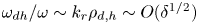 and $k_r \rho _{L,h}\sim O(\delta )$
 , where $\omega _t=v_\parallel /qR_0$
 is the particle transit frequency and $\rho _{d,h}$
 the radial drift, while $q\sim O(\delta ^{-1/2})$
 . The equivalent core particle drift is $k_r \rho _{d,c}\sim O(\delta )$
 , while the finite Larmor effects are of higher order $k_r \rho _{L,c}\sim O(\delta ^{3/2})$
 . Expanding all the perturbed quantities as a series of the powers of $\delta ^{1/2}$
 , like $\delta \phi =\overline {\delta \phi }+\widetilde {\delta \phi }^{(1/2)}+\widetilde {\delta \phi }^{(1)}+\cdots \,$
 , we can solve the system of (2.1) and (2.2) order by order. It was demonstrated by Qiu et al. (Reference Qiu, Zonca and Chen2010) that the adopted ordering yields $\widetilde {\delta \phi }^{(1/2)}=\widetilde {\delta \phi }^{(1)}=\widetilde {\delta \phi }^{(2)}=0$
 , hence to the relevant order $\delta \phi =\overline {\delta \phi }+\widehat {\delta \phi }^{(3/2)}\sin \theta$
 , where $\widehat {\delta \phi }^{(3/2)}$
 is independent of $\theta$
 . The Larmor effects, which come with the Bessel functions $\textrm {J}_0(\lambda )$
 are negligible in the relevant limit for this calculation, but the drift effects should be retained. The energetic particle perturbed distribution then reduces to $\delta H_h=-({e}/{m})({\partial F_{0h}}/{\partial E})\overline {\delta \phi } +\delta H_h^{(3)}$
 . The first term cancels inside the angular bracket on the right-hand side of (2.2) and hence, $O(\delta ^{3})$
 of the quasi-neutrality condition gives (see Qiu et al. (Reference Qiu, Zonca and Chen2010) for details)

where $\omega _G= \sqrt {7/4+\tau }\, v_{th}/R_0$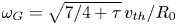 is the GAM frequency, $v_{th}$
 is the core ion thermal velocity, $\tau =T_e/T_i$
 and
and

with $\sigma =v_\parallel /|v_\parallel |$ , $\varLambda =\mu /E$
 and for circulating ions (Qiu et al. Reference Qiu, Zonca and Chen2010),

The equivalent $\overline {\delta H_h^{(3)}}$ term for trapped particles is given in (2.8) of § 2.1.
2.1. Trapped particle treatment
To describe the trapped particles dynamics we use the deeply trapped particle approximation, where the energetic ions are conducting harmonic oscillations in the magnetic mirror of the tokamak field (Chavdarovski & Zonca Reference Chavdarovski and Zonca2009; Zonca & Chavdarovski Reference Zonca and Chavdarovski2009; Chavdarovski & Zonca Reference Chavdarovski and Zonca2014). For large aspect ratio tokamaks $\epsilon =r/R_0 \sim O(\beta ^{1/2})$ the particle parallel velocity is given by $v_{\|}=\theta _{b}\omega _b q R_0 \cos \eta$
 , where $\omega _b= (\epsilon \mu B_0)^{1/2} / {q R_0}$
 is the particle bounce frequency, $B_0$
 is the magnetic field at $r=0$
 , while $\theta _{b}^{2}= 2[E - \mu B_0 (1-\epsilon )] / {\epsilon \mu B_0}$
 is the particle bounce angle, and $\eta$
 is the phase angle of harmonic oscillations on the banana orbit ($\theta =\theta _b \sin \eta$
 ). Further, $\omega _d= k_r v_d \theta _b \sin \eta$
 , $\hat \omega _d=k_r v_d$
 and $v_\parallel \partial _\ell = \omega _b \partial _\eta$
 . We note that (2.4) is valid for trapped particles as long as we maintain the same ordering, hence $\omega \sim \omega _b$
 , $\hat \omega _d / \omega _b\sim O(\delta ^{1/2})$
 and $\theta _{b}\sim 1$
 . Note here that we are using the same ordering for trapped and circulating particles, assuming there is only one energetic species present at the time. If both species are to be accounted for together, they would have different orderings since they have different frequencies of motion and densities.
We pass to the banana orbit centre frame (Tsai & Chen Reference Tsai and Chen1993; Zonca & Chen Reference Zonca and Chen2016) using the substitution $\delta H=\exp ( \textrm {i}({{\hat \omega _d} }/{\omega _b} )\theta _b \cos \eta ) \delta H_b = ( \varSigma _h i^{h} \textrm {J}_h (\lambda _b) \textrm {e}^{-\textrm {i}\eta h} ) \delta H_b$ , where $\delta H_b$
 is the particle distribution function in the new frame and $\lambda _b= \theta _b (\hat {\omega }_d / \omega _b)\sim O(\delta ^{1/2})$
 . Meanwhile, the gyrokinetic equation gives

Due to the ordering, only $h=0,\pm 1$ terms will contribute, i.e. only a constant term and $\omega =\pm \omega _b$
 resonances appear in the final solution, thus linearizing the differential equation as

Dropping the higher order $\sin \eta \cos \eta$ product, it is safe to assume the solution is of a form $\delta H_b=a+b\sin \eta +c\cos \eta$
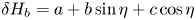 , with $a$
 , $b$
, $b$ and $c$
 being constants to be determined by matching the appropriate trigonometric terms. We go back to $\delta H= (\textrm {J}_0(\lambda _b) +\textrm {i}\lambda _b\cos \eta )(a+b\sin \eta +c\cos \eta )$
 and only keep the terms up to $O(\delta )$
 , which includes the finite orbit width (FOW) effects up to $\lambda _b^{2}$
 . We note again that the Larmor effects are negligible in this ordering $\textrm {J}_0(k_\perp \rho _{Li})=1$
 , while the finite banana width gives $\textrm {J}_0(\lambda _b)\approx 1-\lambda _b^{2}/4$
 and $\textrm {J}_1(\lambda _b)\approx \lambda _b / 2$
 . The orbit averaged $\overline {\delta H}=a \textrm {J}_0(\lambda _b)+\textrm {i} c \lambda _b/2$
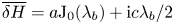 , where we used $\overline {\cos ^{2}\eta }=1/2$
 , $\overline {\cos \eta \sin \eta }=0$
 , $\overline {\cos \eta }=\overline {\sin \eta }=0$
 and we took $\textrm {J}_0^{2}(\lambda _b)\approx 1-\lambda _b^{2}/2$
 to finally get

The first term again cancels out in the quasi-neutrality equation, while the second term is the $\overline {\delta H^{(3)}}$ , which has a similar form with that of the circulating particles in (2.5), with $\omega _b$
 instead of $\omega _t$
 , and some additional terms coming from $\theta _b^{2}$
 . Since $\theta _b\sim O(1)$
 , both terms are of the same order. Note here that the aforementioned approximation of $\textrm {J}_0(\lambda _b)\textrm {J}_1(\lambda _b)$
 is overly simplified and for a better estimate, one should use a Padé approximation. However, simple numerical calculation shows that due to the shape of the distribution function, even this approximation gives very good results for values $\delta \leqslant 0.2$
 .
.
3. Dispersion relation for trapped particles with a bump-on-tail distribution function
The case with circulating energetic ions with a shifted Maxwellian (bump-on-tail) distribution was studied by Zarzoso et al. (Reference Zarzoso, Sarazin, Garbet, Strugarek, Abiteboul, Cartier-Michaud, Dif-Pradalier, Ghendrih, Grandgirard and Latu2013). Here, we will show the derivation and results for trapped particles confined by a narrow cone in velocity space with $- v_\parallel \varDelta \leqslant v_\perp \leqslant v_\parallel \varDelta$ , where $\varDelta =2 \epsilon /(1+\epsilon )$
 . We consider the distribution function:

where $v_0$ is the mean parallel velocity of the beam, while the normalization factor for the trapped particle population is $c_b=n_b(r) \sqrt {\varDelta ^{2} v_2^{2}+v_1^{2}}/(2{\rm \pi} ^{3/2}v_2^{3} v_1 \varDelta )\exp ({v_0^{2}}/{v1^{2}+\varDelta ^{2} v_2^{2}})$
 . Here, $n_b(r)$
 is the beam particle density. This distribution is anisotropic in velocity space, but symmetric in $v_\parallel$
 (see figure 1a). The derivative $\partial f_0/\partial E$
 is an important factor, since it determines the slope of the distribution in energy space and hence the excitation of the mode (Fu Reference Fu2008; Zarzoso et al. Reference Zarzoso, Sarazin, Garbet, Strugarek, Abiteboul, Cartier-Michaud, Dif-Pradalier, Ghendrih, Grandgirard and Latu2013). This particular distribution shows regions of positive and negative gradient depending on the beam velocity $v_0$
 (figure 1b), making the latter a factor in the excitation of the mode. For values of $v_0/v_1$
 below a certain threshold, the function is negative on the entire axis, which makes the mode stable (dashed lines in figure 1b).

Figure 1. (a) Shifted Maxwellian distribution. (b) The energy derivative of the distribution as a function of $v_\parallel$ . (c) The integrand function $L(v_\perp )$
 of (3.2) as a function of $v_\perp$
 and $\alpha _0=v_0/v_1$
 .
.
Inserting $\partial f_0/\partial E$ in (2.4) we obtain (see Appendix A)

where $L(v_\perp )= ({- \exp ({-(v_\perp /v_2)^{2}})}/{v_\perp } )\textrm {I}(v_\perp )$ and $I(v_\perp )$
 is a fairly lengthy function given in the Appendix (A4). Even though the integrand $L(v_\perp )$
 is complicated, it is a smooth function with a pronounced peak (see figure 1c). The figure shows that for values of $v_0$
 lower than a certain threshold discussed below, the function flips the sign, which affects the possibility of excitation of the mode. The integral in (3.2) is not treatable analytically, but it can be easily integrated numerically specially in the upper half of the complex plane. For analytic purposes we will simplify the solution by Taylor expanding to the sixth order (see Appendix A) in $t=\Delta v_\perp /v_1$
 , around $t=0$
 , which is justified for $\varDelta \sim \epsilon$
 and $v_2/v_1 \sim 1$
 . This approximation of $L(v_\perp )$
 shows reasonably close behaviour to the original, and gives familiar analytic functions.
Finally the dispersion relation of EGAMs excited by trapped particles with a bump-on-tail distribution becomes

where the parameters are given by

and

Here, $\alpha _0=v_0/v_1$ , $\alpha _2=v_2/v_1$
 and $\omega _b= v_2 \sqrt {\varDelta }/ (2 q R_0)$
 is the deeply trapped averaged bounce frequency for this anisotropic case, while $Z(x)=1/ \sqrt {{\rm \pi} }\int _{-\infty }^{\infty } \textrm {e}^{-y^{2}}/(y-x)\,{\textrm {d} y}$
 is the plasma dispersion function. The parameters $C_6$
 and $C_8$
 are functions of only $\alpha _0$
 and $\varDelta$
 . Parameter $C_6$
 is the dominant one and hence a major factor in determining the growth rate. For certain values below a threshold, $C_6$
 flips the sign and becomes negative. From the equation for $C_6$
 , we see that near $\epsilon =0$
 this threshold is simply given by $v_0/v_1=\sqrt {2}/2$
 , otherwise it depends on $\varDelta$
 and decreases away from the axis.
It should be noted here that the bounce frequency of the trapped particles $\omega _b$ is somewhat low, so the excitation of the mode is only possible if the frequency is raised relative to the GAM frequency. This implies there can be several other thresholds for the excitation of the mode, aside from the EP density. One of them is the temperature ratio $T_h/T_c$
 , which is also related to $v_2$
 and $\omega _b$
 , since for deeply trapped particles, $\omega _b \propto v_2$
 . A distribution which is wider in perpendicular direction raises the bounce frequency and is more likely to excite the mode, since in this way there will be a larger population with higher frequency in the tail of the distribution that can resonantly interact with the mode. This can be better seen from (3.2) where, due to the form of $L(v_\perp )$
 , the integral depends on the location of the resonant singularity $1/(\omega ^{2}- \omega _b^{2})$
 , relative to the peak of the curve. Hence, if the resonant frequency is too low, the singularity falls to the right-hand side of the peak, while for larger frequency it is on the left side or near the peak. However, if the frequency is too high the singularity falls near $v_\perp =0$
 , where $L(v_\perp )$
 goes to zero.
Equation (3.3) is easily solved numerically using the Newton–Raphson method in complex space. The transcendental functions may generate multiple solutions in the negative complex plane, in which case we only deal with the most unstable branch. Figure 2 shows the frequency and normalized growth rate as functions of the particle density for different values of the beam velocity $v_0$ . Increasing the EP density gives stronger excitation, while the frequency in all cases decreases as expected (Fu Reference Fu2008). The threshold of $n_h$
 here is relatively small due to the assumed negligible continuum and Landau damping. Some threshold of $n_h$
 is expected in a realistic scenario, as is the case with all EPMs (Grad Reference Grad1969; Chen Reference Chen1994). In these plots we set $T_h/T_c=8$
 , $q=1.2$
 , $\epsilon =0.1$
 and $\tau =1$
 . As discussed before larger $v_2/v_1$
 and also larger beam velocity $v_0/v_1$
 increase the drive of the mode. The curve with triangles ($v_0/v_1=1$
 ) shows that approaching the threshold in $v_0=\sqrt {2}/2 \,v_1$
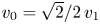 reduces the drive, while the curve with boxes, even though it has a large $\alpha _0=1.7$
 , is closer to the threshold in $v_2/v_1$
 (and equivalently $\omega _b$
 ). This threshold is shown in figure 2(c) for different values of $v_0/v_1$
 . Here, when $v_0/v_1$
 approaches $0.707$
 , $\alpha _2$
 goes to infinity since this is the absolute threshold below which $L(v_\perp )$
 becomes fully negative.

Figure 2. Excitation of EGAM with trapped ion beam with bump-on-tail Maxwellian distribution showing: (a) the real frequency normalized to $\omega _{GAM}$ and (b) growth rate, for different values of $\alpha _0=v_0/v_1$
 and $v_2/v_1$
 . (c) Threshold in $\alpha _2=v_2/v_1$
 as a function of $v_0/v_1$
 .
.
In all cases examined here, there is only one unstable mode and its frequency is lower than the GAM continuum, which is consistent with experimental results for circulating particles (Nazikian et al. Reference Nazikian2008). In conclusion, the shifted Maxwellian provides enough controllable parameters to experimentally create the conditions for the excitation of an EGAM with trapped particles.
4. Slowing-down distribution
For a single pitch slowing-down distribution, $f_0=c_0(r) \delta (\varLambda - \varLambda _0) H_E$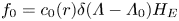 , where $c_0(r)$
 is obtained by normalization as $c_0(r)=\sqrt {2(1-\varLambda _0 B)} n_b(r)/(4 {\rm \pi}B \ln E_b/E_c)$
 and $H_E=\varTheta (1-E/E_b)/(E^{3/2}+E_c^{3/2})$
 . Here, $E_c$
 and $E_b$
 are the energetic ion critical and birth energies, with $E_b \gg E_c$
 . The case for circulating particles was derived by Qiu et al. (Reference Qiu, Zonca and Chen2010). Here we show the result as a comparison with the other distributions and similar works (Zarzoso et al. Reference Zarzoso, Garbet, Sarazin, Dumont and Grandgirard2012). Using

after a lengthy calculation, the EGAM dispersion relation is obtained (Qiu et al. Reference Qiu, Zonca and Chen2010):

Here, $\omega _{ts}= \sqrt {2 E_b (1-\varLambda _0 B)} / (q R_0)$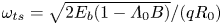 is the EP transit frequency and $N_b=\sqrt {1-\varLambda _0 B} q^{2} n_b (r)/{4 \ln (E_b/E_c) n_c}$
 . The subscript ‘$s$
 ’ in the transit frequency is for the slowing-down case, where $\omega _{ts}$
 is calculated at the birth energy $E_b$
 , while in the Maxwellian case $\omega _{tm}$
 is calculated at the thermal energy $E_{t}=T_h/m_i$
 .
.
Roughly speaking the logarithmic term represents the particle drive and shows an instability threshold $\varLambda _0 B>2/5=0.4$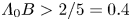 , while the other term gives a shift from the GAM frequency. Detailed solution of the equation usually gives three different roots (similar to Fu Reference Fu2008), the first one of which comes from the GAM branch $\omega =\omega _G$
 , and is found in (4.2) even when there is no drive ($n_h=0$
 ). A pair of solutions with similar frequencies, but different imaginary values, arises from the EP contribution when the value of $n_h$
 is sufficiently high. The frequency and growth rates of all three branches are dependent of the EP density and resonant ion frequency, but there is only one unstable mode (Nazikian et al. Reference Nazikian2008). In figure 3, we show this mode as a function of EP density for different values of $\omega _t$
 and safety factor $q$
 , determined by the radial location of the beam.

Figure 3. Excitation of EGAMs with circulating ion beam with slowing-down distribution showing the real frequency normalized to $\omega _{\textrm {GAM}}$ (a) and growth rate (b).
For $\varLambda _0 B<0.4$ or low $n_h$
 the two EGAM roots become degenerate and show no excitation of a mode. The threshold $\varLambda _0 B>0.4$
 is consistent with results obtained by the gyrokinetic code GYSELA (Grandgirard et al. Reference Grandgirard2008; Zarzoso et al. Reference Zarzoso, Garbet, Sarazin, Dumont and Grandgirard2012), where for values of $\varLambda _0 B\geqslant 0.38$
 there is excitation without limitation on the critical energy. In the other region EGAMs show a threshold in $E_c$
 dependent on $\varLambda$
 and $E_b$
 (Zarzoso et al. Reference Zarzoso, Garbet, Sarazin, Dumont and Grandgirard2012). The assumption made during the derivation here was that $E_c \ll E_b$
 , so (4.2) can not show an $E_c$
 threshold under these conditions, while finite values of $E_c$
 would make (2.5) analytically non-treatable. In (4.1) the first part is always negative, while the second part can be positive or negative, hence the sign of $\partial _E f_0$
 is a function of $E_c$
 and this makes the excitation of the mode dependent on $E_c$
 .
.
Finally, for slowing-down trapped particles we have

which leads to (see Appendix B) the dispersion relation of GAM driven by slowing-down trapped ions:

where $\omega _{bs}= (\epsilon \varLambda _0 B E_b)^{1/2} / (q R_0)$ is the averaged ion bounce frequency. For deeply trapped particles and $\epsilon \ll 1$
 , the pitch angle is restricted to values $(1-\epsilon )/(1+\epsilon )<\varLambda _0 B<1$
 . Although the secular term in (4.4) is cancelled out, the drive term is still present, but shows no excitation since the threshold in $\varLambda _0$
 requires $\varLambda _0 B > 10/9$
 . This result is qualitatively in agreement with Zarzoso et al. (Reference Zarzoso, Garbet, Sarazin, Dumont and Grandgirard2012), where for high $\varLambda _0 B\sim 1$
 the $E_c$
 threshold becomes divergent, although that work considers only circulating particle dynamics, even at high $\varLambda _0$
 .
.
The dispersion relation for EGAMs excited by a not fully slowed-down energetic ion beam was derived by Cao, Qiu & Zonca (Reference Cao, Qiu and Zonca2008) in order to explain the experimental results in the Large Helical Device, where the EGAM appears before the injected neutral beam is fully slowed-down (Ido et al. Reference Ido2015) and the birth energy is higher than the resonant considered in (4.2). The lower energy limit of not fully slowed-down particles is taken to be time variant as $E_L=E_b \textrm {e}^{-\gamma _c t}$ , where $\gamma _c \ll \omega$
 is the slowing-down rate (Cao et al. Reference Cao, Qiu and Zonca2008). The energetic particle square bracket term of (4.2) now has additional terms related to the lower energy limit:

where $\omega _{L}= \sqrt {2 E_L (1-\varLambda _0 B)} / (q R_0)$ . We note here, that the threshold related to the logarithmic term is still $\varLambda _0 B>5/2$
 , and for these values the branch around $\omega _L$
 is excited and can obtain a frequency larger than $\omega _G$
 (see Cao et al. Reference Cao, Qiu and Zonca2008 for details). However, for $\varLambda _0 B<5/2$
 , where the logarithmic terms are stabilizing, the singularity in $\omega \simeq \omega _L$
 can provide for a drive. Hence, in this scenario the EGAM exhibits no threshold in the pitch angle. The drive, regardless of the pitch angle, comes from the positive gradient in energy space at the lower-energy limit of the distribution function and, in that sense, more resembles the bump-on-tail drive, which gives a much bigger growth rate. In the solution for trapped particles (4.4) however, the simple singularity terms cancel out, so this mechanism does not excite EGAMs. Here, we remind the reader that the analytical model for trapped particles has several approximations, therefore we keep open the possibility of excitation with not fully slowed-down trapped particles to be demonstrated by a more rigorous calculation.
5. Single pitch Maxwellian distribution
The single pitch Maxwellian distribution is described by $f_{0h}=c_1(r) \delta (\varLambda - \varLambda _0) H_M$ , where $c_1(r)=\sqrt {2(1-\varLambda _0 B)} n_b(r)/(2 {\rm \pi}^{3/2} B)$
 comes from the normalization and $H_M=1/E_t^{3/2} \textrm {e}^{-E/E_t}$
 . Using here

and again (2.3) and (2.4) gives the local dispersion relation for single pitch Maxwellian circulating particles (see Appendix C):

where

and $N_m={\sqrt {1-\varLambda _0 B} q^{2} n_b(r)}/{2 n_c}$ with $x=\omega /\omega _{tm}$
 and $\omega _{tm}=\sqrt {2 E_t(1-\varLambda _0 B)}/(q R_0)$
 .
.
Here again, when solving (5.2) the transcendental functions generate multiple solutions in the negative complex plane, but only one unstable branch. In figure 4 we show the real frequency and growth rate of the mode as a function of $n_b$ and $q$
 -safety factor. The trends are generally similar to those for slowing-down ions in figure 3 and bump-on-tail in figure 2. The threshold in EP density here is more visible, but still small. The value of the drive is also a consequence of the single pitch angle, and in a realistic case it would be smaller due to the reduced anisotropy. Even though the effect of $\varLambda _0$
 on the EGAMs is not easy to interpret from (5.2), figure 5 shows there is a clear threshold in $\varLambda _0 B$
 which, however, is a function of the other parameters, like $T_h$
 and $q$
 . Careful observation of the thresholds shows that the large part of it is due to the changing of the particle bounce frequency with $\varLambda _0$
 .
.

Figure 4. Excitation of EGAM with circulating ion beam with Maxwellian distribution showing the real frequency normalized to $\omega _{\textrm {GAM}}$ (a) and growth rate (b).

Figure 5. The real frequency normalized to $\omega _{\textrm {GAM}}$ (a) and growth rate (b) versus $\varLambda _0 B$
 for circulating ion beam with Maxwellian distribution showing a threshold in $\varLambda _0$
 .
.
For trapped particles with a single pitch Maxwellian distribution we have the same values for $f_{0h}$ , $c_1(r)$
 and $H_M$
 given above. The local dispersion relation for trapped particles then reads (see Appendix C):

and we have obtained the same threshold $\varLambda _0 B>10/9$ , since the function in the square brackets gives only positive values for positive imaginary frequencies. Hence, this equation too shows no excitation of EGAMs. We should mention here that the asymmetric distribution in the $\pm$
 direction of $v_\parallel$
 does not change the outcome of this analysis. Taking for example the work of Dannert et al. (Reference Dannert, Günter, Hauff, Jenko, Lapillonne and Lauber2008), $f_0 \propto (\exp ({v_\parallel ^{2}/v_{T+}})+\exp ({v_\parallel ^{2}/v_{T-}}))$
 will only change the integration in $v_\parallel$
 and give $1/2[F(x_+)+F(x_-)]$
 , where $F(x)=1/2+x^{2}+x^{3} Z(x)$
 and $x_\pm =\omega /\omega _{t\pm }$
 , with $\omega _{t\pm }$
 having different values in different $v_\parallel$
 directions. However, in both directions the sign of the function $F(x_\pm )$
 is the same, which shows no solutions for trapped particles. The same parallel asymmetry conclusion can also be given for slowing-down particles. The results obtained in this work are strictly valid for deeply trapped particles, but the consistency of the results indicates that the conditions provided by the trapped ions with Maxwellian and slowing-down distributions are not favourable for the excitation of EGAMs.
6. Mode structure
In the previous sections we have assumed the EGAM is not coupled to the continuum, in which case the mode is localized by the Gaussian shape of the ion beam, while its radial width is determined by the FOW of the energetic particles (Fu Reference Fu2008). The safety factor and beam location affect the mode frequency and drive via the values of $N_b$ , $\omega _t$
 and the GAM continuum. This relation is complicated since $N_b$
 increases with $q$
 , but $\omega _t$
 diminishes, while in a realistic tokamak geometry both the GAM and the bounce frequency are affected by the elongation of the magnetic flux surface. Numerical and analytical studies have examined the effects of geometry on the GAM frequency in detail (McKee et al. Reference McKee, Gupta, Fonck, Schlossberg, Shafer and Gohil2006; Zonca & Chen Reference Zonca and Chen2008; Qiu, Chen & Zonca Reference Qiu, Chen and Zonca2009; Zhang & Lin Reference Zhang and Lin2010).
In figure 6 we show the excitation of EGAMs with slowing-down energetic ions using the electrostatic gyrokinetic code GTS (Wang et al. Reference Wang, Lin, Tang, Lee, Ethier, Lewandowski, Rewoldt, Hahm and Manickam2006). This code can perform global nonlinear electrostatic simulations based on a generalized gyrokinetic simulation model using a $\delta f$ particle-in-cell approach, which takes into account the comprehensive influence of many physical effects, including fully kinetic electrons and realistic geometry. Multiple ion species are implemented (background or energetic), following a distribution function of either Maxwellian, shifted-Maxwellian (bump-on-tail), bi-Maxwellian or slowing-down. Numerically, all species are treated on equal footing. In this section, the distribution in pitch angle for slowing-down ions is given by $f_0(\varLambda )=\exp ({-(\varLambda -\varLambda _0)^{2}/(\Delta \varLambda (r))^{2}})$
 , where the width of the distribution is set to $\Delta \varLambda (r) B=0.5$
 and the peak at $\varLambda _0 B=0.2$
 . The critical energy $E_c$
 is above the excitation threshold, and the distribution gives (mostly) circulating particles. The mode is localized approximately around the same radial location as the beam, with small deviation which is allowed by the FOW of the energetic particles. An exception to this is when the particle beam is streaming along the axis and a mode is excited by the beam's radial tail off-axis at $x=0.4$
 , where the conditions for excitation are met, which shows again that modes on the axis are more difficult to excite (Chavdarovski et al. Reference Chavdarovski, Schneller, Qiu and Biancalani2017; Schneller et al. Reference Schneller, Fu, Chavdarovski, Wang, Lauber and Lu2017). In this case, the energetic particle density around $x=0.4$
 is small, but the excitation is possible due to the FOW effects. When the energetic particles are sharply peaked on the axis we get no excitation. In figure 6 different growth rates depending on the location of the mode are obtained, which confirms that the optimal location (here $x=0.4$
 ) for excitation of an EGAM is away from the edge (Fu Reference Fu2008).

Figure 6. Scan of the EP density peak radial position $r/a$ (a) and the resulting change in the EGAM radial structure (b).
Figure 7 shows excitation of the mode with beams of different radial widths at the same location $x=0.5$ and with the same parameters used in figure 6. In both cases the mode structure is identical, the real frequency changes slightly, but the growth rate is strongly affected and is bigger for the wider beam. This is not a general conclusion, since there are several factors that determine the growth rate. The wider beam drives a lower frequency mode, which is related to a higher growth. This is most likely due to the changing of the resonant frequency with the change of the location of the energetic particles. Additionally, the wider distribution has more particles at the inside location, which shows better drive of the mode and lower frequency in figure 6. Another issue is that the relative orbit width compared with the mode structure plays an important role in determining the drive, and the orbit width is a function of the radial distribution and location.

Figure 7. (a) Different radial extensions of the EP distribution function (dashed lines) and the resulting EGAM structure (solid lines), and (b) their growth.
In figure 8 the effect of the peak $\varLambda _0$ on the mode structure is shown. It should be noted that, while the analytical models take a single species, here there is a continuous distribution of particles in $\varLambda$
 , such that some of the particles are trapped and some circulating. When $\varLambda _0 B=0.8$
 most of the particles are trapped and show no excitation, consistent with the theoretical prediction of § 4. For lower $\varLambda _0 B$
 the circulating population is dominant, while the critical energy $E_c$
 is set above the excitation threshold. The particles with higher $\varLambda _0$
 have larger orbit width, which gives the mode with $\varLambda _0 B=0.5$
 a slightly wider mode structure than the mode with $\varLambda _0 B=0.2$
 . Figure 8(b,d) shows that the width of the particle distribution in energy space only slightly affects the mode shape, location and width, again due to different orbit sizes, with the wider beam (in $\varLambda$
 ) giving a slightly wider structure.

Figure 8. (a) Scan over the peak of the beam pitch angle for $\varLambda _0 B= 0.2, 0.5, 0.8$ and (c) resulting EGAM mode structure. (b) Scan over the width of the EP pitch angle distribution function: $\Delta \varLambda = 0.2, 0.5, 0.7$
 and (d) the mode structure.
7. Summary
In this work we have derived the local dispersion relations of energetic-particle-induced geodesic acoustic modes (EGAMs) for both circulating and trapped particle beams with single pitch angle slowing-down and Maxwellian distributions, as well as a bump-on-tail distribution for trapped particles. The dispersion relations for trapped particles are a novel result, as are the results for circulating particles with a single pitch Maxwellian distribution. In the case for trapped particles with a bump-on-tail distribution, the excitation of the mode shows a threshold in the density ratio of hot versus core ions. Additionally, we obtain a threshold in the mean velocity of the ion beam $v_0/v_1=\sqrt {2}/2$ , as well as a threshold in the hot ion bounce frequency determined by the $v_2/v_1$
 ratio, as a function of $v_0/v_1$
 . The drive provided by the trapped ions with a bump-on-tail distribution is shown to be stronger than that for slowing-down circulating particles. For trapped particles with a slowing-down distribution the equation shows no excitation of EGAMs, which is also the case for single pitch Maxwellian, as well as Maxwellian with $\pm$
 asymmetry in a $v_\parallel$
 distribution.
For circulating ions with a single pitch Maxwellian distribution, we find more than the three branches that appear in the slowing-down case. However, only one of them can be unstable and that branch, identified in experiments as an EGAM, has a frequency below the GAM continuum. The dispersion relations are solved numerically for different values of the safety factor and the resonant particle frequency. The solutions show that the real frequency and growth rate of the mode are dependent of the pitch angle, the energetic particle density and their resonant frequency $\omega _t$ , similar to the case for slowing-down ions. Simulations for slowing-down circulating ions with the gyrokinetic code GTS show that the structure and growth of the mode are dependent on the beam location and width, in real and energy space.
The results presented here are consistent with the experiments, but also connect well with the previously obtained analytical results.
Acknowledgements
Useful discussions with Z. Qiu, P. Lauber, G.Y. Fu, Z. Lu and F. Zonca are kindly acknowledged. The views and opinions expressed herein do not necessarily reflect those of the European Commission.
Editor Francesco Califano thanks the referees for their advice in evaluating this article.
Funding
This work was part of Max Planck-Princeton (MPPC) Center for Plasma Physics study 2015–2017. Work done by the coauthor A.B. has been carried out within the framework of the EUROfusion Consortium and has received funding from the Euratom research and training program 2014–2018 and 2019–2020 under grant agreement number 633053. This work was supported by R&D Program through Korean Institute of Fusion Energy (KFE) funded by the Ministry of Science and ICT of the Republic of Korea (KFE-EN2141-7).
Declaration of interests
The authors report no conflict of interest.
Appendix A. Derivation for trapped particles with bump-on-tail distribution
Placing the derivative

in (2.4) and limiting the integral to the trapped population in velocity space, we obtain

where

Integrating over $v_\parallel$ gives a rather complicated function of $v_\perp$
 and $v_0$
 :
:

Here, $P(v_\perp )= \exp ({-(\Delta v_\perp - v_0)^{2}/v_1^{2}}) - \exp ({-(\Delta v_\perp +v_0)^{2}/v_1^{2}})$ , $Q(v_\perp )= \exp (-(\Delta v_\perp - v_0)^{2}/v_1^{2}) + \exp ({-(\Delta v_\perp +v_0)^{2}/v_1^{2}})$
 and $R(v_\perp )=\textrm {erf}(\Delta v_\perp /v_1-v_0/v_1)+\textrm {erf}(\Delta v_\perp /v_1-v_0/v_1)$
 , where the error function is defined as $\textrm {erf}(x)=({2}/{\sqrt {{\rm \pi} }} )\int _0^{x} \textrm {e}^{-t^{2}}\,\textrm {d}t$
 . The integrand of (A2) can be written as $L(v_\perp ) /(v_\perp ^{2}-{\omega ^{2} q R_0 }/{2\sqrt {\varDelta }})$
 where
where

Expanding in Taylor series to the sixth order in $t=\Delta v_\perp /v_1<1$ ,
,

with $v_p=v_0/v_1$ , and using the usual expansions for $\exp ({-(t - v_p)^{2}})$
 and $\exp ({-(t + v_p)^{2}})$
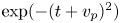 , we get

Here, we have omitted terms higher than $v_\perp ^{8}$ and used the notation $C_6$
 and $C_8$
 for the respective constants. The integral with $C_6$
 is solved using the replacement $y=v_\perp /v_2$
 and
and

which is related to the plasma dispersion function $Z(x)$ (see Chavdarovski Reference Chavdarovski2009, p. 105). The second integral can be obtained from $\textrm {Y}_6$
 as
as

Placing these results into (2.3) gives the dispersion relation (3.3).
Appendix B. Derivation for slowing-down distribution
The dispersion relation follows from (2.3), where $\overline {\delta n_h}$ is obtained from the integral in (2.4):

with $A={\rm \pi} c q^{2}k_r^{2}\delta \bar {\phi }/(\sqrt {2}B \varOmega _i)$ . The terms in the square brackets give two separate double integrals. The first one containing $\partial H_E/\partial E$
 is straightforward when integrating over $\delta (\varLambda -\varLambda _0) d\varLambda$
 , but requires partial integration in the energy space: $\int M(E) (\partial H_E/\partial E) \,\textrm {d}E= H_E M(E)\mid _{0}^{\infty }-\int H_E (\partial M(E)/\partial E)\,\textrm {d}E$
 , where for brevity we have placed all the other quantities in the $E$
 -dependant $M(E)$
 function. Due to the Heaviside function and $E_c \ll E_b$
 we have

The other term of the partial integration, with the assumption $E_c \ll E \sim E_b$ and some manipulation, becomes

where all of the constants are extracted outside making both integrals elementary. The second part of (B1) is solved by partial integration in $d\varLambda$ as
as

where the first term vanishes for $\varLambda _0 \in (a,b)$ , with a and b being the limits of $\varLambda _0$
 , which differ for circulating and trapped particles. The derivative

gives the same type of integrals over $E$ as previously obtained. Hence, when all the terms are integrated and grouped together we obtain (4.4).
Appendix C. Derivation for Maxwellian distribution
When a single pitch Maxwellian distribution of energetic particles is used the derivative

again gives two integrals with delta function, where the second one additionally requires partial integration. The first integral reduces to

and the energy part is then solved using the replacement $y^{2}=E/E_t$ and (A8). After the partial integration of the second term in (C1) we get two separate integrals, the first one of which has the form

(see Chavdarovski Reference Chavdarovski2009, p. 105), while the other

where $x=\omega /\omega _t$ and we have reduced Y to (A8) using the Leibnitz rule. Applying the derivative $Z_x=-(1-xZ(x))$
 inside $\partial /\partial x \, \textrm {Y}_6$
 , and placing everything in (2.3), after reorganizing the terms we obtain the dispersion relation (5.2).
For trapped Maxwellian particles we can write

where the first term is elementary, while the second term is solved as above, with an additional integral

appearing in the partial integration, which is then reduced to (C3).


