


NOMENCLATURE
- a 0
-
speed of sound at sea level in ISA conditions [m/s]
- alt
-
aircraft altitude [ft]
- ACARS
-
Aircraft Communications Addressing and Reporting System
- ADS-B
-
Automatic Dependent Surveillance – Broadcast
- APM
-
aircraft performance model
- ASL
-
altitude above sea level [ft]
- ATM
-
Air Traffic Management System
- BADA
-
Base of Aircraft Data
- CLFPL
-
child flight plan resulting from a genetic operation
- CDO
-
Continuous Descent Operations
- CFP
-
corrected flight plan
- CG
-
centre of gravity
- CI
-
cost index value [kg of fuel/min]
- C f_dist
-
segment length correction factor function of geometric altitude relative to the sea level altitude [–]
- deg
-
degrees
- EOC
-
end of cruise
- EST
-
Eastern Standard Time
- flight_time
-
flight time [h]
- fpm
-
feet per minute [ft/min]
- fuel_burn
-
fuel burned for a flight along a flight trajectory [kg]
- ft
-
feet
- FAA
-
Federal Aviation Administration
- FMS
-
Flight Management System
- FT_TO_NM
-
ft to n.m. conversion factor [n.m./ft]
- g 0
-
gravitational acceleration [m/s2]
- GA
-
genetic algorithm
- GDPS
-
Global Deterministic Prediction System
- GRIB2
-
atmospheric data file format
- GS
-
ground speed [Kn]
- h
-
hour
- hPa
-
hectopascal [100N/m2]
- h geom
-
geometric altitude relative to sea level [ft]
- IAS
-
indicated air speed [Kn]
- IATA
-
International Air Transport Association
- ICAO
-
International Civil Aviation Organization
- IDLE
-
idle thrust engine setting
- ISA
-
international standard atmosphere conditions
- J
-
joule (SI unit of energy) [N m]
- kg
-
kilogram (SI unit of mass)
- Kn
-
speed in knots [NM/h]
- K
-
kelvin (SI unit of temperature)
- lat
-
latitude position for an aircraft or a waypoint location [deg]
- lon
-
longitude position for an aircraft or a waypoint location [deg]
- LARCASE
-
Laboratory of Research in Active Control, Avionics, and Aeroservoelasticity
- LAX
-
Los Angeles Airport code
- m
-
metre (SI unit of distance)
- min
-
minute
- MACH
-
Mach number [–]
- MCMB
-
maximum climb thrust engine setting
- MCRZ
-
maximum cruise thrust engine setting
- MMO
-
maximum operating MACH speed limit [–]
- MSL
-
mean sea level altitude – actual elevation above mean sea level
- n.m.
-
nautical mile
- N
-
newton (SI unit of force)
- NM
-
grid node position along the orthodromic route
- NORT
-
number of grid nodes along the orthodromic route
- NCFP
-
non-corrected flight plan
- NP
-
nondeterministic polynomial-time problem
- ORT
-
orthodromic route
- p S
-
atmospheric static pressure [Pa]
- p s0
-
standard atmosphere sea level atmospheric static pressure in ISA conditions [Pa]
- Pa
-
pascal (SI unit of pressure) [N/m2]
- P i
-
parent i for a crossover operation
- P ix
-
section x (1 or 2) of parent i
- PA
-
pressure altitude [ft]
- qc
-
dynamic pressure [N/m2]
- rpm
-
rotations per minute
- R
-
real gas constant for air [m2/(K s2)]
- RDPS
-
Regional Deterministic Prediction System
- R earth
-
Earth’s radius [n.m.]
- RTA
-
Required Time of Arrival [h]
- RUC
-
Rapid Update Cycle
- s
-
second (SI unit of time)
- segm_len
-
sea level length of a lateral flight profile segment, according to the selected segment type (orthodromic or loxodromic) [NM]
- segm_hdg
-
departure angle, relative to geographic north, for a lateral flight profile segment, according to the selected segment type (orthodromic or loxodromic) [deg]
- Sj
-
step j of the crossover operation, along the orthodromic grid route
- SI
-
international system of units of measurement
- SLA
-
sea level altitude – the reference altitude, taken to be the 0 altitude [ft]
- t
-
time [h]
- T
-
air temperature [K]
- T 0
-
sea level standard air temperature [K]
- TAS
-
true airspeed [Kn]
- TBO
-
Trajectory-Based Operations
- TC
-
total cost for flight along an evaluated flight profile [kg of fuel]
- TEM
-
Total Energy Model
- TLA
-
thrust lever angle [%]
- TOC
-
top of climb
- TOD
-
top of descent
- UAS
-
Unmanned Aerial Systems
- UAV
-
Unmanned Aerial Vehicles
- UTC
-
Coordinated Universal Time
- VMO
-
maximum operating IAS speed limit [Kn];
- W U
-
wind speed component along the geographic north axis [Kn]
- W V
-
wind speed component along the geographic east axis [Kn]
- WGS84
-
World Geodetic System 1984 – ellipsoid earth model
- WPT
-
waypoint
- ZHR
-
Zurich Airport code
-
 ${\alpha _{CD}}$
-
aircraft climb/descent angle [deg]
-
${\alpha _{CRB}}$
-
aircraft crabbing angle relative to segment heading [deg]
-
${\alpha _{Segm}}$
-
flight segment angle relative to geographic north [deg]
-
$\gamma $
-
adiabatic index for air [–]
-
$\theta $
-
temperature ratio [–]
- 4D
-
four-dimensional space (latitude, longitude, altitude and time)


1.0 INTRODUCTION
According to ICAO forecasts(1,2) , the future annual growth of passenger and cargo traffic, up to 2035, is estimated to be approximately 4.3% and 3.9%, respectively, which will result in a doubling of the number of passengers by 2037(3). This reality requires better flight planning, navigation and airspace management strategies and tools to facilitate safe and efficient routing of aircraft through an increasingly crowded airspace.
The expected air traffic increase highlights the need to identify optimal flight trajectories that are adapted for each origin–destination pair, aircraft model (performance) and load, atmospheric conditions, and navigation constrains (restricted areas, altitude and/or speed constraints, time constraints, etc.). Better flight planning would result not only in better use of airspace but also in a reduction of fuel consumption, with a direct impact on greenhouse-gas emissions and, therefore, on the environment. Additionally, the resulting operational cost reductions would benefit aircraft operators, and the economy in general.
An improvement of flight planning performance could be achieved by several methods, individually or in combination, such as:
Better aircraft performance models, which would allow a better and quicker estimation of an aircraft’s flight trajectory (space and time evolution) and fuel consumption; For example, a new fuel burn model for constant altitude and speed flight, proposed by Dancila et al. (Reference Dancila, Botez and Labour4), computes the fuel burned in a selected flight time, and the flight time necessary to burn a selected fuel quantity, faster and with greater precision than existing methods. This model can be used, for example, to determine the earliest moment when a step climb is possible;
Better atmospheric data forecasts, which would yield atmospheric data closer to that encountered by aircraft during flight; For example, the tailored descent forecast wind method, proposed in ref. (Reference Bronsvoort, Mcdonald, Potts and Gutt5), was designed to improve the predictability of Continuous Descent Operations (CDO) flight trajectories computed by Flight Management System (FMS) platforms. This method generates tailored wind forecasts based on the selected landing procedure, and on high-resolution regional forecasts;
New navigation strategies, which could yield greater flexibility in selecting a flight trajectory that is better adapted to the flight mission. By implementing the Trajectory-Based Operations (TBO) paradigm(Reference Torres and Delpome6,Reference Cate7) , it would be possible for each aircraft to fly along a flight trajectory that is adapted to the specific flight, and atmospheric conditions;
New optimisation strategies, which would identify faster, and more precisely, globally optimal or near-optimal flight plans/trajectories.
The flight trajectory optimisation process can be approached from two main directions as a function of the objective of the optimisation. In a first approach, the optimisations can be performed at a global level (airspace), in Air Traffic Management System (ATM) platforms. In this case, the main focus is to increase the airspace throughput while maintaining safe operations: ensure the minimum space and time separation between aircraft(Reference Rodionova, Sibihi, Delahaye and Mongeau8,Reference Chaimatanan, Delahaye and Mongeau9) , and eliminate or reduce the potential for flight trajectory conflicts(Reference Matsuno and Tsuchiya10). The optimality of a flight trajectory, at aircraft level, is not considered or is secondary to the main objective stated above.
A second approach concerns the optimisation of a flight trajectory at the aircraft level, according to a selected criterion (e.g. fuel burn, flight time, or operational costs minimisation) and the imposed navigation constraints (e.g. altitude and/or speed constraints along the flight track, time constraints, etc.). An aircraft flight trajectory optimisation can be conducted on-board (during the flight), in an FMS platform, or on the ground, in the flight-planning phase (before the flight). The requirements for on-board optimisation methods are stricter, due to the limited computational power available and the standards for on-board equipment certification (deterministic algorithms).
Generally, a flight trajectory optimisation problem can be defined as an optimal control/guidance problem, where the objective is to identify a control law that will guide the aircraft along the optimal flight trajectory(Reference Soler, Olivares and Staffetti11–Reference Bonami, Olivares, Soler and Staffetti17), or as a search problem, where the optimal flight profile is obtained using search algorithms.
In a study presented in ref. (Reference Di Vito, Corraro, Ciniglio and Verde18), the authors conducted a review of on-board flight trajectory optimisation algorithms, strategies and patents for 2D, 3D and 4D trajectory optimisations. The analysis focuses on identifying the features of the proposed methods, their strengths and weaknesses, and suggests new directions of investigation based on the analysed solutions. Yu and Zhang(Reference Yu and Zhang19) presented an extensive survey of path planning methods, with a focus on flight planning for Unmanned Aerial Systems (UAS).
Multidisciplinary optimisation methods(Reference Ceruti, Voloshin and Marzocca20,Reference Ceruti, Fiorini, Boggi and Mischi21) can be applied for trajectory optimisation when there are multiple competitive/contradictory requirements (e.g. performing an assigned mission while avoiding restricted airspace/threats).
Zillies et al. (Reference Zillies, Kuenz, Schmitt, Schwoch, Mollwitz and Edinger22) analysed the achievable improvement in flight efficiency in European airspace if flight trajectories were to be optimised for actual atmospheric conditions (air temperature and winds). Their study considers a flight at constant altitude and speed, where ‘candidate’ routes are constructed based on the orthodromic route between the limits of the segment to be optimised. A route is composed of a limited number of waypoints (a maximum of six). A Dijkstra search algorithm is applied iteratively to identify the best node among five equally spaced nodes constructed at the halfway point between the current node (at the current iteration) and the destination, until the remaining segment length is less than 100 n.m. The authors observed that detours resulting from following better wind conditions led to savings in fuel and time compared with orthodromic routes.
Ceruti and Marzocca.(Reference Ceruti and Marzocca23) devised a method for optimising the flight trajectory of two airships, modelled by Bézier curves, using a particle swarm optimisation algorithm. The two airships, one of which is cruising (denoted ‘cruiser’) while the other is climbing from the ground (denoted ‘feeder’), must perform an in-flight docking manoeuvre. The optimisation algorithm identifies the parameters of the Bézier curves and the target speed at the docking point so that, at the docking point, the two trajectories are tangent, the two airships have identical speeds and the total energy required for the manoeuvre is minimal.
Qu, Zhang and Zhang(Reference Qu, Zhang and Zhang24) proposed a novel two-step flight path optimisation method for Unmanned Aerial Vehicles (UAVs) flying in hostile airspace. In a first step, a Dijkstra search algorithm identifies the shortest route through the airspace, determined by selecting nodes of a grid obtained by 3D Delaunay triangulation of the airspace. In a second step, the shortest route identified in the first step is optimised using an artificial potential field method to take into account weather, aircraft dynamics and threats.
Casado et al. (Reference Casado, Goodchild and Vilaplana25) studied the influence of the uncertainty of aircraft performance parameter estimation for the climb, cruise and descent phases of the flight on the safety, efficiency, and capacity of the ATM system. They used a stochastic aircraft performance model generated on the basis of an aircraft performance degradation model, in conjunction with Monte Carlo simulations, to determine the sensitivity of the trajectory prediction error to the aircraft performance model uncertainty for each phase of the flight, and the parameters that are most influenced by these uncertainties.
An aircraft behavioural model(Reference Gillet, Nuic and Mouillet26) based on analysis of historical flight data addresses the need to use realistic aircraft behaviour in ATM flight simulations to better predict air traffic conditions.
A method to generate estimations of wind prediction uncertainties, presented by Lee et al. (Reference Lee, Weygandt, Schwartz and Murphy27), analysed each forecast data point of a Rapid Update Cycle (RUC) forecast, and computed their average wind components values as well as the standard deviations (considered as wind uncertainty). That work analysed the effects of wind uncertainties on aircraft trajectory predictions by comparing the along-track differences between a simulated flight with predicted winds, and a simulated flight where uncertainties were added to the forecasted winds.
Reference(Reference Dancila and Botez28) addresses the problem of selecting the maximal optimal geographic area for flight trajectory routing, while bounding the maximum total ground distance to a selected value. The authors presented a new method for selecting an ellipsoidal geographic area for routing, where the parameters of the ellipsoid are based on the origin and destination of the flight and the selected maximum flight trajectory length.
A method for reducing the number of flight segment performance calculations made during the flight trajectory optimisation, proposed by Dancila and Botez(Reference Dancila and Botez29), constructs in advance, for each phase of the flight (climb, cruise and descent) and cruise altitudes, a set of performance data for vertical path segments that cover the aircraft’s flight envelope. The flight segment performance data are constructed based on the specific optimisation problem: origin–destination pair, aircraft load, set of speeds, and a set of selected landing weights.
Franco and Rivas(Reference Franco and Rivas30) analysed the optimal control problem for a minimum-cost cruise at constant altitude, where the initial and final speeds are imposed. The authors studied the singular arc section of the bang-singular–bang solution and the cost variation as a function of flight time for three wind conditions and two cost index values, as well as for flights with RTA constraints. For flights with RTA constraints, the optimal flight corresponds to the CI value for which the minimum fuel profile yields the RTA.
Chamseddine, Zhang and Rabbath(Reference Chamseddine, Zhang and Rabbath31) presented a method for re-planning the flight trajectory for a formation of UAVs when one of the UAVs has failures. The objective is to identify a new flight trajectory and control laws that take into account the limited capabilities of the faulty UAV (i.e., that does not exceed the limitations imposed for the actuators), maintain the formation structure and the desired separation between vehicles, and minimise the energy consumption.
A 3D trajectory planning method(Reference Zhou, Duan, Li and Di32) based on differential evolution uses a chaotic search, performed around the best solution identified for each generation, to improve the search results and escape locally optimal solutions. A flight trajectory optimisation method proposed by Patrón et al. (Reference Berrou and Botez33) performs optimisation of a flight plan using a genetic algorithm. The lateral flight profiles are constructed by selecting nodes from a grid formed by five parallel tracks (the planned flight track and four parallel tracks). First, vertical flight profile optimisation for the climb phase is performed along the planned flight track by evaluating all the speed combinations considered for this phase. Next, for the cruise phase, five parallel tracks (two on each side of the original trajectory) are divided into n segments to form a routing grid for the cruise phase. A first optimisation using a genetic algorithm identifies the optimal cruise flight track for the planned vertical flight profile. Then, an optimisation of the vertical flight profile identifies the optimal vertical profile for the optimal flight track identified in the previous step. Finally, the descent phase is optimised by exhaustive evaluation of the descent speed combinations. The flight trajectory method proposed in ref. (Reference Botez34) is similar to that presented in ref. (Reference Berrou and Botez33), with the difference that the lateral and vertical flight profiles are optimised simultaneously.
The optimisation method proposed by Murrieta-Mendoza et al. (Reference Murrieta-Mendoza, Beuze, Ternisien and Botez35) defines the vertical flight trajectory optimisation as a discrete combinatory problem (discrete values for the flight speed and altitude), modelled as a decision tree, and uses the Beam Search Algorithm to identify the optimal flight profile. Their method visits the nodes of the decision tree and, at each visited node, uses an optimistic cost evaluation heuristic to prune the decision tree to eliminate the non-optimal branches, thereby reducing the number of profile calculations. In ref. (Reference Murrieta-Mendoza, Beuze, Ternisien and Botez36), a search space reduction method is applied before using the Beam Search Algorithm, which can reduce the search space by 50% and thereby the execution time.
Murrieta-Mendoza et al. (Reference Murrieta-Mendoza, Botez and Bunel37) presented the results of a lateral and vertical flight trajectory optimisation with RTA constraints using an Artificial Bee Optimisation algorithm. The lateral flight profiles generated during the optimisation were constructed based on a dynamic routing grid. A Golden Search algorithm then optimises the MACH speed for the optimal profile, identified by the bee optimisation algorithm, to obtain a speed profile with values within a predetermined set. New constant speed segments are introduced to observe the RTA constraints.
The 4D flight trajectory optimisation method proposed by Murrieta-Mendoza et al. (Reference Murrieta-Mendoza, Hamy and Botez38) models the flight trajectory as a 3D grid (lat, lon and alt), where the aircraft flies at the ECON speed and, at each node, the aircraft may advance only to neighbouring grid nodes. The Mach speed profile is then optimised along the 3D profile using an Ant Colony Optimisation algorithm, so that the RTA constraint is observed (4D).
This paper presents a flight trajectory optimisation method based on genetic algorithms (GA). The proposed method is designed to determine the ‘best’ flight trajectory for the selected origin–destination pair, aircraft model (performance characteristics) and load, atmospheric conditions, candidate flight profile characteristics, optimisation criteria and imposed constraints. This method is intended to be used by flight operators, in the planning phase (before a flight), or for flight plan update/change during a flight, on ground-based computers. The resulting optimal flight plans will then be uploaded to the aircraft.
2.0 METHODOLOGY
This section is structured as follows: The first sub-section (2.1) presents the concepts related to flight trajectory optimisation. The next sub-sections describe the aircraft performance model used in this study (2.2), the atmospheric data model used in the flight trajectory performance calculations (2.3) and the elements of a flight trajectory (2.4) (i.e. the characteristics of the set of candidate flight trajectories evaluated in the optimisation, and the methodology used to construct them). The following two sub-sections present the methodology used for computing the flight performance parameters for a flight trajectory through accelerated flight performance calculation (2.5) and the proposed optimisation method based on the genetic algorithm (2.6). Finally, the last sub-section (2.7) presents the flight data used for constructing the test cases and the reference flight plan (to evaluate the performance of the proposed method).
2.1 Flight trajectory optimisation
The objective of a flight trajectory optimisation process is to identify the optimal flight profile for a particular optimisation problem defined by the aircraft model (flight performance and envelope limitations), initial aircraft load and fuel quantity, initial and final trajectory points data and constraints (crossing time at the initial point, initial and final aircraft geographic locations, altitudes and speeds), navigation constraints, atmospheric conditions and selected optimisation criteria. The optimisation criterion is, in general, the minimisation of a cost function (e.g. minimisation of fuel burn, total cost, flight time, etc.). However, it can also be a maximisation of the cost function (e.g. maximum loitering time, etc.).
An aircraft flight trajectory can be decomposed into two components:
A lateral flight profile, represented by the projection of the flight trajectory onto the Earth’s surface; and
A vertical flight profile, defined by the evolution of the aircraft’s flight parameters (e.g. altitude, speed, vertical speed/rate of climb or descent/angle of climb or descent, acceleration/deceleration, load factor, etc.) along the lateral flight profile.
In still air (no wind), International Standard Atmosphere (ISA) conditions and the absence of navigation constraints, the optimal lateral flight profile is the orthodromic route (the shortest route on the sphere/ellipsoid) between the initial and final point of the flight plan under optimisation. The optimal vertical flight profile is specific to the aircraft model, aircraft weight and the cost function selected as optimisation criterion. When real atmospheric conditions are taken into account, i.e. wind and non-standard atmospheric temperature conditions, it may be advantageous to deviate from the orthodromic route, and to perform altitude and speed changes to benefit from more advantageous wind and air temperature conditions.
A flight trajectory optimisation process is conducted by successively evaluating flight trajectory profiles from a set of candidate flight profiles, in each step retaining as solution the ‘best’ flight profile relative to the cost function and criterion set as objective for the optimisation. The optimisation process can be conducted for only one or for both components of the flight profile. In the former case, one of the components of the flight plan (lateral or vertical) is common to all the candidate flight plans while the other component is different for each candidate flight plan. In the latter case, both flight plan components can change.
The methodologies used to generate the set of candidate flight plans and select the flight plan to be evaluated at each step of the optimisation process are heuristic methods, selected depending on the specific optimisation problem, selected cost function, constraints, etc.
For flight plans with navigation constraints (e.g. altitude, time, etc.), the constraints take precedence relative to the flight profile’s optimality. If the constraints are not satisfied, the flight plan is considered non-valid and rejected. Similarly, a flight plan is considered non-valid and is rejected if:
The flight profile generated based on the flight plan yields aircraft flight parameters that are beyond the aircraft’s flight envelope boundaries; or if
The flight along the resulted flight profile requires more fuel than is available.
The particular optimisation problem considered in this paper is specific to the cases where:
The flight plans do not have navigation constraints;
Both the lateral and vertical components of the flight plan can be modified during the optimisation; and
The objective is to minimise the total cost for the flight.
The total cost for a flight is calculated as the sum of the fuel cost and the operational costs, which are proportional to the flight time and expressed as fuel quantity (kg of fuel). A detailed presentation of the total cost function, and the elements that contribute to it, can be found in refs. (Reference Robertson39–Reference Dejonge and Syblon41).
The total cost is calculated using the following formula:
 \begin{equation}TC = fuel\_burn + CI\; \times \;fligh\_time\; \times \;60\end{equation}
where:
TC is the total cost, expressed in terms of fuel quantity [kg of fuel];
fuel_burn is the fuel burned for the flight along the evaluated flight profile [kg of fuel];
flight_time is the flight time for the flight along the evaluated flight profile [h]; and
CI, the cost index, is a constant (specific to each airline, aircraft type and route) that converts the flight time into operational costs expressed in terms of fuel quantity [kg of fuel/min].
The CI value adjusts the optimisation to obtain a trade-off between the fuel consumption and the flight time; the larger the CI value, the greater the weight that is attributed to the reduction of the flight time in the optimisation process.
If CI = 0, the optimisation criterion becomes fuel burn minimisation. When the CI value reaches a maximum value (e.g. 999), specific for a platform, the optimisation criterion becomes flight time minimisation.
The flight performance and aircraft dynamics (e.g. fuel burn, flight time, speeds, accelerations, travelled distances, etc.) parameters are calculated by performing an accelerated simulation of the flight along the evaluated flight profile. These calculations are performed using an Aircraft Performance Model (APM) specific to the aircraft type, the atmospheric data along the flight profile (wind and air temperature), the aircraft’s configuration parameters (mass, engine thrust setting, landing gear, flaps and speed brake positions, etc.) and the flight profile’s data (speed, climb/descent angle, bank angle, load factor, etc.).
The method presented in this paper does not take into account any navigation constraints (such as restricted areas or airways, Required Time of Arrival (RTA), etc.), and adopts the TBO/‘free flight’ paradigm; the aircraft is thus free to fly along the trajectory that is best suited for the origin–destination pair, atmospheric conditions, aircraft performance and load.
2.2 Aircraft performance model (APM)
The APM used in this study is the Base of Aircraft Data (BADA) version 4.0(42), developed and maintained by Eurocontrol. The APM provides specific aircraft type data (i.e. mathematical models and the related coefficients for the aircraft parameters, valid aircraft flight configurations, flight envelope limitations, etc.), a methodology for calculating the aero propulsive forces acting on the aircraft, the aircraft motion as a result of these forces (equations based on the Total Energy Model (TEM)) and the associated fuel burn. An overview of the BADA APM can be found in refs. (42–Reference Nuic, Poles and Mouillet43), ref (44) (for BADA version 3.7) and ref. (Reference Nuic45) (for BADA version 3.8). Specific information regarding the BADA version 4.0 APM can be obtained from Eurocontrol(42) upon request, and is subjected to a licence agreement.
The set of input parameters used in the calculation of the flight performance parameters, and in the aircraft’s evolution along the flight path, their range of valid values and units of measurement, are specific to the APM. As an example, the input parameters can be:
Aircraft configuration parameters: aircraft mass, centre of gravity position, landing gear position, flaps/slats position, spoilers/speed brakes position, etc.;
Engine parameters: These parameters are specific to the engine type. For a jet engine, they can be the Thrust Lever Angle (TLA), engine fan speeds, etc.;
Atmospheric conditions: air temperature and wind; and
Flight trajectory parameters: altitude, speed, acceleration/deceleration, bank angle, load factor, climb/descent angle, rate of climb/descent, etc.
A flight trajectory is composed of a succession of elementary flight profile types (e.g. constant-speed cruise segment, acceleration/deceleration cruise segment, constant-speed constant-TLA climb/descent, constant-TLA constant-rate-of-climb accelerated climb segment, etc.). Depending on the type of flight profile evaluated, some of the parameters presented above are input parameters while others are output parameters (resulting from the flight performance calculations). For example, for a cruise segment at constant altitude and constant speed, a selected speed (an input parameter) will require a specific engine thrust setting and thus fuel burn rate (an output parameter) to maintain the selected speed and altitude. Conversely, a selected engine thrust setting (an input parameter) will determine the speed and fuel burn rate (output parameters). The flight trajectory performance calculation model, developed using the APM, implements a specific performance calculation function for each elementary flight profile type and set of output parameter(s) of interest.
2.3 Atmospheric data
Atmospheric conditions have an important influence on aircraft flight performance characteristics and dynamics. The air temperature influences the engine performance and, as a result, affects the available thrust, the maximum altitude for a selected speed, the minimum and maximum speeds at a selected altitude, the fuel burn rate, etc. The aircraft speed along the flight trajectory is defined in terms of the Indicated Air Speed (IAS) or MACH number. The aircraft’s aerodynamic characteristics are functions of the True Airspeed (TAS), which is the aircraft’s speed relative to the mass of air. The aircraft’s evolution along the flight trajectory is a function of the ground speed (GS), which is the aircraft’s speed relative to the ground. The TAS value, computed as a function of the active speed value and its type (IAS or MACH), is affected by the air temperature and static pressure values.
For MACH speeds, the TAS is expressed only as a function of the air temperature(Reference Botez46):
 \begin{equation}TAS = M\sqrt {\gamma RT} = M\sqrt {\gamma R{T_0}} \sqrt {\frac{T}{{{T_0}}}} = M{a_0}\sqrt \theta \end{equation}
where:
M is the Mach number;
-
$\gamma $
= 1.4 is the adiabatic index for air;
R = 287.05J/kg/K is the universal gas constant for dry air;
T is the air temperature [K];
T 0 = 288.15K is the standard air temperature at Sea Level Altitude (SLA), considered as 0ft, in International Standard Atmosphere (ISA) conditions;
-
${a_0} = \sqrt {\gamma R{T_0}} =340.29\;{\rm{m}}/{\rm{s}}$
is the speed of sound at SLA in ISA conditions; and
-
$\theta = \;\frac{T}{{{T_0}}}$
is the air temperature ratio relative to the ISA SLA air temperature.


For a flight in the IAS speed mode, in the subsonic regime, when air compressibility effects are neglected, the relationship between the TAS and the IAS is described in ref. (Reference Botez46):
 \begin{equation}TAS = {a_0}\sqrt {5\theta \left[ {{{\left( {\frac{{{q_c}}}{{{p_s}}}+1} \right)}^{3.5}} - 1} \right]} \end{equation}
where q c is the dynamic pressure computed for the IAS speed at the SLA in ISA conditions:
 \begin{equation}{q_c} = {p_{s0}}\left\{ {{{\left[ {1+0.2{{\left( {\frac{{IAS}}{{{a_0}}}} \right)}^2}} \right]}^{3.5}} - 1} \right\}\end{equation}
and:
a0 is the speed of sound at SLA and in ISA conditions;
-
$\theta $
is the air temperature ratio relative to the ISA SLA air temperature;
p S is the static air pressure at the flight altitude (pressure altitude);
p S0 = 101,325Pa is the static air pressure at SLA (0 ft) in ISA conditions; and
IAS is the scheduled speed that is converted to TAS.

An aircraft flight trajectory is composed of segments defined by a set of fixed geographic points (waypoints (WPTs)) selected between the departure and destination points. In still air, in the absence of winds, the aircraft’s heading is the segment heading at the aircraft location and the GS is equal to the TAS. In the presence of winds, for the aircraft’s trajectory to follow the segment’s track, the aircraft’s heading must change (a process called ‘crabbing’) so that the GS vector’s direction, resulting as the vectorial summation between the TAS and wind vector, is oriented along the segment’s heading at that location. The GS value and the aircraft’s crabbing angle (
 ${\alpha _{CRB}}$
. ) relative to the segment heading are computed using the wind triangle algorithm(Reference Botez46). Their expressions are:
${\alpha _{CRB}}$
. ) relative to the segment heading are computed using the wind triangle algorithm(Reference Botez46). Their expressions are:
 \begin{equation}\left\{ {\begin{array}{*{20}{l}}{GS}&=&{\left( {{W_V}cos{\alpha _{Segm}} + {W_U}sin{\alpha _{Segm}}} \right) + \sqrt {{{\left( {TAScos{\alpha _{CD}}} \right)}^2} - {{\left( {{W_V}sin{\alpha _{Segm}} - {W_U}cos{\alpha _{Segm}}} \right)}^2}} }\\{{\alpha _{CRB}}}& = &{\frac{{180}}{\pi }arcsin\left( {\frac{{{W_V}\sin {\alpha _{Segm}} - {W_U}\;cos{\alpha _{Segm}}}}{{TAS}}} \right)}\end{array}} \right.\end{equation}
where:
GS is the ground speed;
-
${\alpha _{CRB}}\;$
is the aircraft’s crabbing angle relative to the segment heading;
TAS is the true airspeed;
W V and W U are the wind speed components along the geographic north and east axes;
-
${\alpha _{CD}}$
is the aircraft’s climb/descent angle; and
-
${\alpha _{Segm}}$
is the flight trajectory segment’s heading, relative to geographic north, at the aircraft’s location.


Equations (3), (4) and (5) show that the air temperature and the wind affect the TAS and the GS values. This influence, in turn, affects the flight performance (lift, drag, required thrust, etc.) and the flight trajectory/dynamics: the flight times along and/or the lengths (ground distances) of the segments composing the flight profile (climb/descent distances, climb/descent speeds, rate of climb/descent, etc.). For an accurate estimation of the aircraft’s trajectory and flight performance parameters, it is therefore necessary to perform the calculations using atmospheric conditions that are as close as possible to the real conditions encountered during flight.
The atmospheric conditions (i.e. air temperature and wind) are constantly changing, and at each time instance, their values are different, being functions of the geographic location (latitude and longitude) and the altitude of the point where they are measured. The atmospheric data used in flight performance calculations are generated based on prediction data issued by meteorological agencies. Due to the chaotic nature of the atmosphere and to the limitations of the atmosphere models used in the prediction process, atmospheric data predictions issued by the meteorological agencies may differ from the actual atmospheric conditions occurring at the prediction location (latitude, longitude and altitude) and time. The magnitudes of the prediction errors vary as a function of the forecast type (global or regional) and resolution (forecast grid size), the time of year, the time of day (day or night), region, how far ahead in time the prediction is made, etc.(Reference Lee, Weygandt, Schwartz and Murphy27,Reference Stohl47–Reference Cole, Green, Jardin, Schwartz and Benjamin50) .
The atmospheric data used in this study are a Global Deterministic Prediction System (GDPS)(51) forecast issued by Environment Canada in GRIB2(52,53) data file format. GDPS is a global level forecast, issued twice a day, at 00h and 12h Coordinated Universal Time (UTC), that provides atmospheric data forecasts at the nodes of a 4D grid (latitude, longitude, pressure altitude and time) in the following format:
On a latitude–longitude map projection, available with two grid resolutions: 0.25° × 0.25°(54) and 0.6° × 0.6°(55);
At a fixed set of 27 isobaric levels (pressure altitudes); and
The forecasts are made at 3-h intervals, for 240h for the 0.25° × 0.25° grid, and 144h for the 0.6° × 0.6° grid.
Therefore, each atmospheric parameter of interest (air temperature and wind) can be computed as a function f(lat, lon, static air pressure, t) of the location of the point (latitude, longitude and pressure altitude) and the time instant for which they are evaluated.
Graphical illustrations of a GDPS atmospheric data forecast (air temperature and winds) on a 0.6° × 0.6° grid, issued by Environment Canada on 25 February 2019, at 12:00 UTC, for 25 February 2019, at 21:00 UTC, at a pressure altitude of 300hPa (30,065f.), cropped to a geographic area delimited by latitude 10ºN and 75ºN and longitude 130ºW and 30ºE, are presented in Figs 1 and 2.

Figure 1. Example of air temperature forecast data issued by Environment Canada on 25 February 2019 at 12 UTC for 25 February 2019 at 21 UTC, at 300hPa pressure altitude.
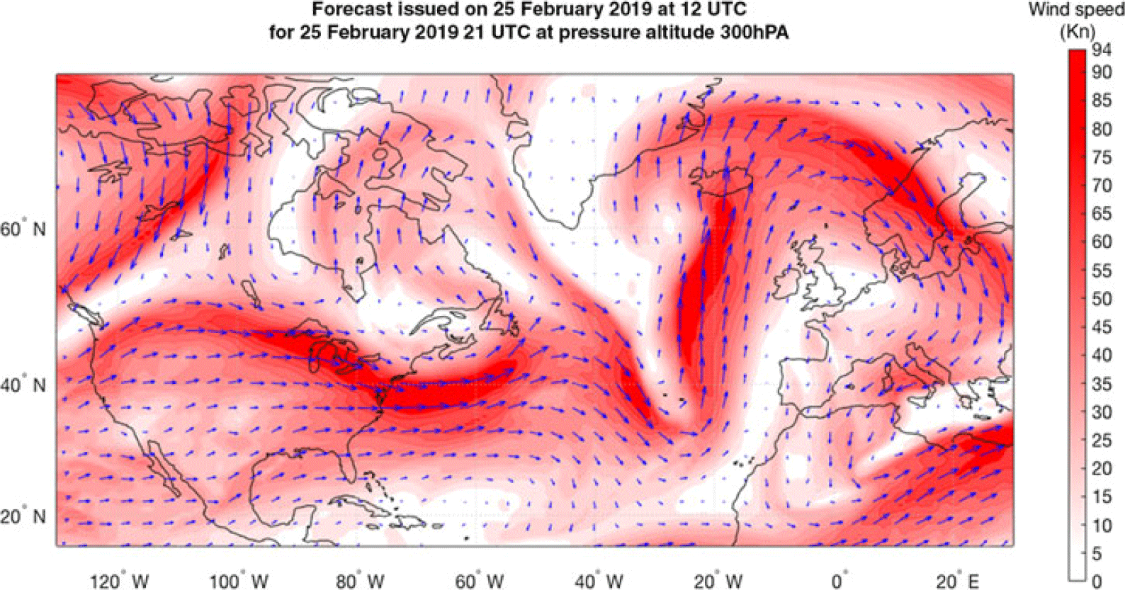
Figure 2. Example of wind forecast data issued by Environment Canada on 25 February 2019 at 12 UTC for 25 February 2019 at 21 UTC, at 300hPa pressure altitude.
The atmospheric parameters at a point other than a node of the forecast’s 4D grid are computed by interpolation. The method selected in this study for atmospheric parameter interpolation is ‘4D linear interpolation’, as predominantly used in flight trajectory optimisation algorithms and flight trajectory performance calculations(Reference Stohl47,Reference Schwartz, Benjamin, Green and Jardin48,Reference Stohl, Wotawa, Seibert and Kromp-Kolb56–Reference Wickramasinghe, Harada and Miyazawa61) . More complex interpolation methods (such as quadratic, bicubic, spline, polynomial, etc.) are potentially more precise but are slower than 4D linear interpolation. These interpolation methods have often been used in the literature(Reference Soler, Olivares and Staffetti11,Reference Soler, Olivares and Staffetti12,Reference Soler, Olivares, Staffetti and Bonami62,Reference Fukuda, Shirakawa and Senoguchi63) , on ground-based platforms, in conjunction with regional atmospheric data forecasts and near-horizon flight profile predictions such as the descent phase of a flight/CDO(Reference Jin, Cao and Sun64). Regional atmospheric data predictions, such as RDPS(65) and RUC(Reference Schwartz, Benjamin, Green and Jardin48), are short-time forecasts issued for a reduced geographic area, but updated at a much higher rate and being more precise.
2.4 Flight trajectory/flight plan
Generally, an aircraft flight trajectory can be very complex, limited only by the aircraft’s performance capabilities (flight envelope limitations), the abilities of the pilot and the required workload (if a manoeuvre is performed in manual mode), or the FMS/autopilot capabilities. Additional constraints are imposed by navigation and safety regulations, and passenger comfort.
In the fields of flight trajectory planning and optimisation, ATM, and FMS, a flight trajectory is defined by a flight plan(Reference Altus66,67) that contains all the information regarding the intended evolution of the aircraft, in a concise and standard format. The flight plan contains all the information necessary to predict the precise space–time evolution of the aircraft. The description of the flight trajectory using a standard format is a result of the necessity to:
Reduce the complexity of flight profiles;
Easily construct the flight trajectory in ATM and FMS platforms, based on the submitted/selected flight plan;
Implement the functionalities required for the calculation of the aircraft flight performance parameters and aircraft flight dynamics, along a selected trajectory, through accelerated simulation, in order to:
-
Compute flight performance parameters (e.g. fuel burn, flight time, etc.);
-
Ensure that the flight parameters (e.g. altitude, speed, etc.) remain within the aircraft’s flight envelope limits;
-
Evaluate the aircraft’s position relative to the flight plan, and follow the planned trajectory (FMS);
-
Evaluate possible conflicts with other aircraft within the same airspace region (ATM); and
-
Validate the flight plan relative to imposed navigation constraints, fuel requirements, etc.
-
As mentioned in Section 2.1, an aircraft flight trajectory can be decomposed into two components:
A lateral flight profile, representing the projection of the flight trajectory onto the Earth’s surface; and
A vertical flight profile, defined by the evolution of the aircraft’s flight parameters along the lateral flight profile.
Accordingly, a flight plan has a lateral and a vertical component, corresponding to the two components of the flight trajectory.
2.4.1 Lateral flight plan description and resulting lateral flight profile
The lateral flight plan defines the segments composing the lateral flight profile:
The sequence of waypoints (WPTs) that define the lateral flight profile segments overflown by the aircraft (geographic locations defined by pairs of latitude and longitude coordinates); and
The lateral flight profile segment type(s): loxodromic or orthodromic(Reference Lenart68) (Fig. 3).
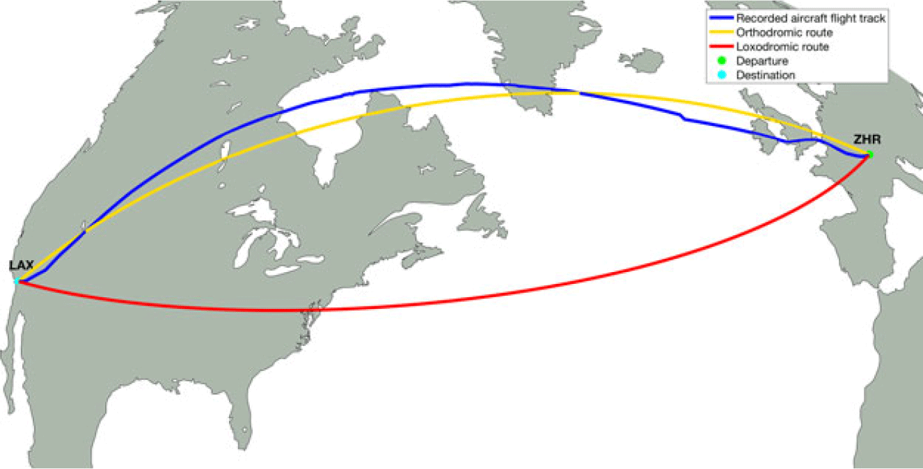
Figure 3. Illustration of orthodromic and loxodromic routes, and a recorded flight track(69) between Zurich (ZHR) and Los Angeles (LAX).
A loxodromic segment (represented by the red line in Fig. 3) has the property that, at every point on the segment, the departure heading required to advance along the segment is constant. However, a loxodromic segment is not the shortest route between two points on a sphere or ellipsoid.
An orthodromic segment (represented by the yellow line in Fig. 3) is the shortest route between two points on a sphere/ellipsoid (the geodesic or great circle that connects two geographic points). On an orthodromic route, the segment heading is not constant; it varies from the departure WPT (beginning of the segment) to the arrival WPT (end of the segment).
Although the orthodromic route between two geographic locations is the shortest flight distance between two points, aircraft do not necessarily follow accurate orthodromic routes due to air traffic constraints, atmospheric conditions (to avoid strong head winds and/or turbulence), navigation constraints, etc. The blue line in Fig. 3 illustrates the lateral flight profile of a real flight, flight SWR40 between Zurich (ZHR) and Los Angeles (LAX), on 25 February 2019, retrieved from the FlightAware web site(69).
Two consecutive WPTs from the lateral flight plan define a flight profile segment and, together with the segment type information, determine the segment’s SLA length, and the departure and arrival headings (the angle relative to geographic north) at each point along the segment. Conversely, given the initial WPT of a segment and the segment type, the departure heading from the initial WPT and the SLA for a point of interest, it is possible to compute the geographic coordinates of the point of interest and the arrival heading at this point.
For a loxodromic segment, the calculations of various parameters (SLA length, the segment heading, the coordinates of a point situated at a given SLA distance, etc.) are performed using the rhumb line equations(Reference Carlton-Wippern70) for the Earth model (spherical or ellipsoid). For orthodromic segments, the calculations are performed differently as they are functions of the Earth model used: spherical trigonometry for a spherical earth model, and Vincenty’s formulas(Reference Karney71) for an ellipsoid Earth model.
The segment’s length at the aircraft’s flight altitude is obtained by multiplying the SLA distance by a correction factor calculated as:
 \begin{equation}{c_{f\_dist}} = \;\frac{{{R_{earth}}\; + \;{h_{geom}}\; \times \;FT\_TO\_NM}}{{{R_{earth}}}}\end{equation}
where:
-
${c_{f\_dist}}$
is the segment length correction factor with altitude;
R earth = 3440.1n.m. is the Earth’s radius;
h geom is the aircraft geometric altitude relative to sea level, in ft; and
FT_TO_NM = 16.457884 × 10⁻⁵n.m./ft is the ft to n.m. conversion factor.

As an example, for a geometric altitude of 36,000ft,
 ${c_{f\_dist}}$
= 1.0017222.
${c_{f\_dist}}$
= 1.0017222.
2.4.2 Vertical flight plan description and resulting vertical flight profile
A vertical flight plan defines, in a succinct form, the aircraft’s altitude–speed evolution along the lateral flight profile, and specifies the locations (WPTs) along the lateral flight plan segments where changes occur in the planned vertical flight profile parameters (e.g. altitudes and speeds), as well as their new values. In this paper, it is assumed that the vertical flight plan defines the locations along the lateral flight plan where the changes are initiated (e.g. at the beginning of an acceleration/deceleration to a new speed, at the beginning of a climb/descent to a new flight altitude, etc.). A vertical flight plan (profile) can be decomposed into seven main phases: take-off, initial climb, climb, cruise, descent, approach and landing. Each flight phase can include one segment or a succession of vertical flight plan segments.
The vertical flight profile, generated by the vertical flight plan, is obtained by applying accelerated flight performance calculations (see Section 2.5). Each flight plan segment is decomposed in a succession of ‘standard’ type segments, i.e. segments in which the control parameters and the mathematical models describing the aircraft’s evolution (the dynamic and the status parameters) do not change (e.g. a constant-altitude constant-speed segment, a constant-altitude acceleration segment, a climb segment at constant speed and constant climb angle, a climb segment at constant speed and rate of climb, etc.).
The set of parameters that define a vertical flight plan segment are specific to the flight segment type. The values of a vertical flight plan segment parameter can be specified:
Explicitly, provided as input;
Implicitly, when the parameter value:
-
Is ‘inherited’ and does not change relative to the value it had at the end of the previous vertical flight plan segment; or
-
Results from the flight performance parameter calculation (e.g. the geographic location where a constant-altitude acceleration/deceleration segment ends, the geographic location where a climb segment ends, the altitude and geographic location where an accelerated climb segment ends, etc.).
-
The climb and descent sections are flown at ‘scheduled speed’, defined as an [IAS, MACH] speed pair. The speed mode switch (between IAS and MACH) takes place at the crossover altitude, defined as the altitude where the TAS computed from the IAS, described by Equation (3), is equal to the TAS computed from the MACH speed, given by Equation (2). The IAS speed is in effect below the crossover altitude, and the MACH speed is above the crossover altitude. The reason for the speed mode change at the crossover altitude is that a climb at constant IAS speed beyond the crossover altitude would result in a MACH speed beyond the maximum MACH operating speed limit (MMO); similarly, a descent at constant MACH below the crossover altitude would result in an IAS speed beyond the maximum operating speed limit (VMO). An example of a climb speed profile is presented in Fig. 4, where the flight plan starts when the aircraft is at an altitude of 10,000ft and speed of 250Kn IAS, and defines a climb segment at [300Kn IAS, 0.80 MACH] to the cruise altitude (33,000ft). Following the accelerated flight performance calculations, the resulting flight profile is composed of three segments:
An acceleration in climb, from 250Kn to the scheduled speed climb IAS (300Kn), which starts at 10,000ft and ends at an altitude that is a function of the aircraft performance parameters, such as weight, etc.;
Climb at constant IAS (300Kn) to the crossover altitude (30,594ft); and
Climb at constant scheduled speed MACH (0.8) to the cruise altitude (33,000ft).

Figure 4. Example of altitude–speed profile for the climb phase of a flight.
It should be noted that the positions along the lateral flight plan segments (lateral flight profile) where the accelerated climb segment and the constant-speed climb segments end are determined during the accelerated flight performance calculations. These positions are not only dependent on the flight plan speeds but also dependent on the aircraft flight performance characteristics, weight and atmospheric conditions.
The structure of a descent altitude–speed profile is similar to that of a climb altitude–speed profile, except that the evolution along the profile is reversed.
The cruise phase is composed of a succession of constant-altitude and climb (step climb) segments flown at MACH speed (constant-speed, acceleration or deceleration segments). Generally, descent segments (step descents) are not employed, as the aircraft performance is better at higher altitudes, and repeated sequences of step climbs and step descents result in an increased number of pressure change cycles on the airframe, thereby increasing maintenance costs.
Figure 5 shows an example of an altitude profile for the climb, cruise and descent phases of a real flight (flight Swiss SWR40, from Zurich to Los Angeles, flown on 25 February 2019), as retrieved from FlightAware(69). The altitude profile data presented in Fig. 5 have been selected to show the trajectory for altitudes above 10,000ft.

Figure 5. Example of altitude profile for flight SWR40, Zurich to Los Angeles, on 25 February 2019. Data for altitudes above 10,000ft, as retrieved from FlightAware(69).

Figure 6. Illustration of the TOC, EOC and TOD positions along the altitude flight profile.
The transition between the climb and cruise sections of the flight trajectory occurs at the Top of Climb (TOC), the point where the aircraft reaches the cruise altitude. The transition between the cruise and descent sections of the flight trajectory occurs at a point denoted as the Top of Descent (TOD), where the aircraft initiates the descent. Another important point along the vertical flight profile is the End of Cruise (EOC), situated in the cruise section of the vertical flight profile, at a pre-set sea level distance from the final point of the descent. The EOC is the point along the flight trajectory beyond which the accelerated flight performance calculation function performs the calculations in ‘descent’ mode, which is a methodology specific to the descent phase of the flight. A more detailed presentation regarding the positions of the TOC, EOC and TOD along the lateral flight profile is provided in the next sub-section (2.5). Figure 6 illustrates the TOC, EOC and EOD positions along the altitude flight profile.
2.5 Accelerated flight performance calculation
The aircraft model developed based on the APM provides a set of functions that compute the flight performance parameters and the aircraft dynamics for each ‘standard’ flight profile segment type that can be used to construct a flight trajectory, as well as to evaluate the flight parameters relative to the aircraft’s flight envelope.
The evolution of the aircraft along the selected flight trajectory, the flight performance and the aircraft status parameters are computed iteratively, segment by segment, starting from the initial point, by accelerated simulation:
The flight trajectory is constructed as a succession of ‘standard’ segments;
Each segment of the flight trajectory is decomposed into sub-segments (integration steps);
The parameter along which a segment is decomposed into sub-segments (time, distance, altitude) depends upon the segment’s type;
The integration step size (sub-segment decomposition step size) is chosen as a result of a tradeoff between the estimated result precision and computation time. Larger step sizes would result in a smaller number of sub-segments and, therefore, faster calculations. However, this would also reduce the accuracy of the results;
For each sub-segment, the specific parameters are calculated in a point on the sub-segment (situated along the decomposing parameter dimension) using the appropriate evaluation function, aircraft configuration, atmospheric conditions, etc.;
The performance parameters for the sub-segment are obtained by integration: the parameters returned by the function are multiplied by a factor computed based on the integration step size; and
The aircraft’s state and configuration parameters, and its position along the lateral flight profile, are updated. The new values become the input data for the trajectory performance calculation on the next sub-segment.
At each step, the aircraft performance parameters, its state, position and dynamics are validated relative to the flight envelope limitations (such as altitude and speed), quantity of fuel on board, flight trajectory, navigation constraints, etc.
The methodology used for constructing the flight trajectory profile and computing the performance parameters is presented in ref. (Reference Schreur72). The flight trajectory construction and the flight performance parameter calculation start from the initial point of the flight plan (initial geographic location and altitude), with the initial aircraft status parameter values (zero fuel weight, fuel quantity, centre-of-gravity position, speed, climb angle, bank angle, etc.), and the time instance when the aircraft crosses the initial point of the flight plan. The climb phase is computed first, followed by the cruise phase. The TOC location, namely the point where the aircraft reaches the cruise altitude, is determined by the climb profile calculation module. The cruise phase calculations stop at a pre-set sea level distance from the final point of the flight plan (EOC), heuristically selected so that it is further away from the destination than the beginning of the descent flight profile (TOD). The aircraft weight and crossing time at the final point of the flight profile (flight plan) are then estimated using a heuristic, and the estimated values are used to construct the descent flight profile. The descent flight profile is constructed in reverse order (backwards integration), from the final point of the descent flight plan to the TOD, at the cruise altitude and speed. At this stage, the geographic location of the TOD and the aircraft crossing time at the TOD are known. Finally, the performance parameters are computed for the last segment of the cruise flight profile, delimited by the EOC and TOD. Validation of the estimated aircraft weight and crossing time at the end of the flight profile is performed by comparing their values obtained at the TOD, viz. the values obtained from the descent profile calculations with the values obtained from the cruise profile calculations. If the aircraft weight and/or the crossing time difference are larger than selected threshold values, considered acceptable, then the estimated values at the end of the descent are corrected (based on the difference obtained for the parameter value) and the process is started again for a new decent profile computation, EOC to TOD profile calculation and comparison between the obtained values. This process stops when both the time difference and the aircraft weight difference are smaller than the selected threshold values. Figure 7 shows a flowchart of the accelerated flight profile calculation process.
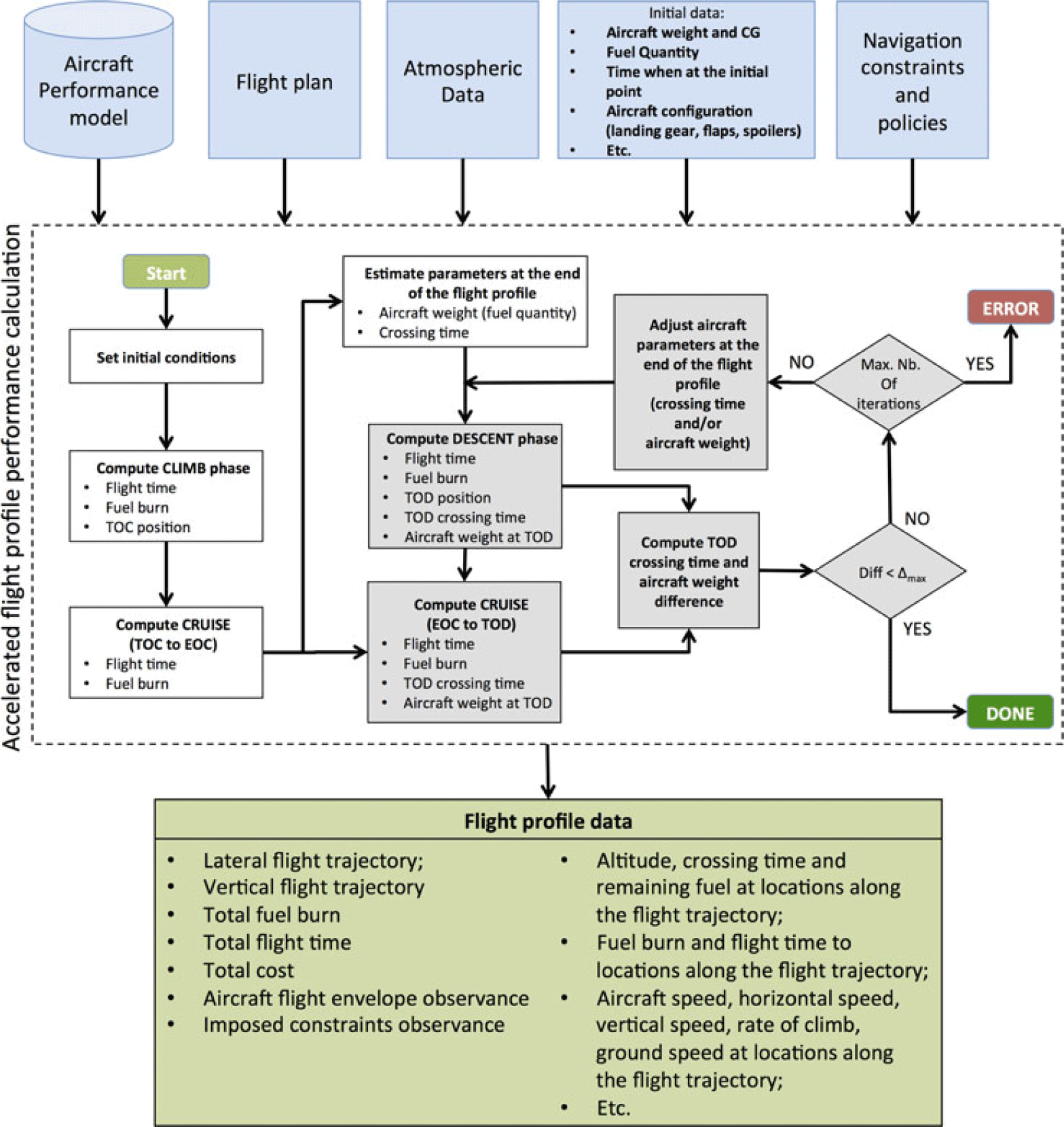
Figure 7. Accelerated flight profile calculation process flowchart.
Navigation constraints (such as altitude, speed, RTA, etc.), assigned at different points along the flight path, are validated by comparison with their corresponding values resulting from the flight performance calculations.
2.6 Optimisation method
The optimisation method presented in this paper is intended for flight trajectory optimisation (Section 2.4) where modifications are made to both the lateral and vertical flight profiles. For a specific optimisation problem, defined by:
Aircraft model (flight performance data), load (weight) and onboard fuel quantity;
Geographic locations of the initial and final points of the flight trajectory;
Aircraft flight altitude and speed at the beginning and at the end of the flight profile under optimisation;
Navigation policies such as: Climb at Maximum Climb (MCMB) TLA, IDLE descent, climb/descent mode (e.g. vertical speed, climb/descent angle, rate of climb/descent), etc.;
Selected values for the range of cruise altitudes, and the maximum deviation from the orthodromic route between the beginning and the end of the flight trajectory under optimisation; and
Optimisation criterion: minimisation of fuel burn, flight time or total cost.
The algorithm implementing the proposed optimisation method identifies the ‘optimal’ flight plan, viz. the combination of lateral (Section 2.4.1) and vertical (Section 2.4.2) flight plans that minimises the selected cost function.
The optimisation problem presented in this paper considers a discrete/combinatorial optimisation with a very large number of candidate solutions, determined by the characteristics of the family of candidate flight plan solutions (Sections 2.6.1 and 2.6.2). Some of the parameters that are used in the calculations (e.g. the atmospheric conditions, aircraft performance model) are defined by piecewise functions. The evolution of the aircraft is described by piecewise functions due to the decomposition into sub-segments in which the mathematical model that describes the evolution of the aircraft and flight parameters do not change (see Section 2.5, which describes the methodology used to compute the flight performance for a flight plan). Moreover, the total cost is expressed by a complex non-linear function due to the relationship between the parameters that determine the total cost (fuel burn, flight time) and the input parameters: aircraft weight, flight plan parameters (altitude and speed flight profile) and atmospheric conditions. The total cost of a flight segment depends not only on its selected parameters but also on the parameters of previous flight profile segments. The aircraft weight, altitude and crossing time at the beginning of a segment result from the fuel burn and flight time on previous segments (and thereby their flight profile characteristics). This fact affects the aircraft’s performance characteristics and the atmospheric conditions encountered on the segment, which affect the fuel burn and flight time and, as a consequence, the segment’s total cost. This optimisation problem might have multiple local minima and many (‘near’-)optimal solutions. For these reasons, the optimisation method described in this paper is based on genetic algorithms.
Due to the random nature of genetic algorithms, the optimality of the solution is not guaranteed; it is expected that the solution will be a ‘near-optimal’ flight plan. Multiple runs of the optimisation algorithm, for an identical optimisation problem, yield different ‘optimal’ solutions.
The proposed optimisation method starts by defining the families (‘templates’) of lateral and vertical flight plans from which the candidate flight plans (the combination of lateral and vertical flight plans) can be selected and evaluated during the optimisation process. Then, a genetic algorithm iteratively selects random new candidate flight plans, from the candidate set or by applying genetic operators (‘crossover’ and ‘mutation’) on pairs of selected candidates, and computes the flight performance parameters (through accelerated simulation), and the cost. The genetic operators are applied in such a way that the resulting flight plans after applying the genetic operators are themselves members of the candidates’ set.
The first sub-section presents the methodology used for constructing the set of candidate lateral flight plans, and the configuration parameters that determine their characteristics. The next sub-section describes the methodology employed for constructing the family of vertical flight plans, and the configuration parameters that determine their characteristics. The last sub-section presents the implementation of the genetic algorithm used in the optimisation.
2.6.1 Lateral flight profile routing grid and candidate lateral flight plan construction
This sub-section presents the methodology used for constructing the set of lateral flight plans that can be selected as components of the flight plans evaluated in the optimisation. The definition of the set of lateral flight plans starts from the assumption that the lateral flight plan is composed by a succession of segments, each of which is delimited by two geographic locations (WPTs) and is one of two possible types: orthodromic or loxodromic. Another assumption made in this study is that the WPTs delimiting the lateral flight plan segments and, therefore, the aircraft’s lateral flight trajectory are restricted to a selected geographic area. It is also assumed that the set of WPTs that delimit the segments of a lateral flight plan are selected from a ‘grid’ (routing grid), in which each segment is delimited by two adjacent WPTs from the grid.
The set of lateral flight plans is, therefore, defined by:
The geographic area within which the flight plan WPTs can be selected;
The methodology used to construct the routing grid, which defines the set of WPTs that delimit the flight plan segments;
The type of the segments (orthodromic or loxodromic) composing the lateral flight plan; and
The methodology used for selecting, from the routing grid, the set of WPTs that define the succession of segments of the lateral flight profile.
In this study, the lateral flight profile is composed of orthodromic segments. Each segment is characterised by:
An SLA length;
The headings required to advance along the segment: at the initial WPT of the segment (departure heading) and at points along the segment; and
The heading when arriving at the final WPT of the segment.
The segment’s length, the departure and arrival headings and the segment headings at points along the segment are computed using the Vincenty’s formulae(Reference Karney71) and the WGS84 ellipsoid Earth model(Reference Janssen73).
In this study, the routing grid, and thus the geographic area to which the set of flight plans are restricted, is defined based on the orthodromic route (ORT) between the initial and final WPTs of the trajectory under optimisation. The routing grid is constructed as an ‘orthogonal’ grid. First, a number of equidistant WPTs are generated along the ORT. Then, from each such WPT along the ORT, an orthodrome perpendicular to the ORT is constructed, and new routing grid WPTs are generated along this orthodrome. The new WPTs are equidistant, placed symmetrically, on both sides of the ORT, up to a maximum deviation relative to the ORT. An illustration of the routing grid construction is presented in Fig. 8.

Figure 8. Example of routing grid construction.
The first step in constructing the routing grid is to select the configuration parameters for the grid:
The maximum distance between the WPTs generated along the ORT;
The maximum deviation from the ORT; and
The distance between WPTs on the normal to the ORT.
It is assumed that the aircraft always moves to a new WPT situated at a (routing grid) step along the ORT track, and at a maximum number of grid steps across. The lengths of the segments along and across the orthodromic track, and the number of waypoint steps ‘across’ the ORT, are chosen such that each segment, constructed as presented above using waypoints selected from the grid, represents an integration step (has a maximum length that is below the maximum length of a computation step) for the flight performance estimation function.
These parameters can also be used to refine the optimisation process, as smaller distances produce a finer grid, which can yield profiles that are ‘better’ adapted to the atmospheric conditions, although this would result in a large increase in the number of ‘candidate’ profiles to explore.
Given that, at each step, the aircraft moves to a new WPT situated at one grid step along the ORT and at a selected maximum number of steps across the ORT, the routing grid starts at the initial WPT, with no WPTs across the ORT. Then, at each step along the ORT, the number of WPTs across the ORT increases by the selected maximum number of steps across, up to the maximum number of deviations resulting from the selected maximum deviation from the ORT and the lateral deviation step size. Similarly, at the other end, the number of WPTs across the ORT decreases, at each step along the ORT, by the maximum number of lateral deviation steps, until it reaches the final point of the grid (the final WPT of the flight) with no WPTs across the ORT. Figure 9 presents an illustration of a routing grid.

Figure 9. Example of a routing grid.
The lateral flight plans, generated as candidates in the optimisation, are random routes that traverse the routing grid, where the succession of WPTs must follow the rules set out above. One method for generating the lateral flight plan is to select the set of WPTs successively, one step along the orthodromic route at a time (with each new WPT being situated one step further along the orthodromic route). The domain of valid steps along the normal to the orthodromic route (the range of lateral steps that would end in a grid WPT) is determined, at each step, and the new WPT deviation is selected randomly, from the set of valid deviations. Tests showed that such a method yields zigzag lateral flight plans (e.g. the red flight track in Fig. 10), which result in flight trajectories that are not in accordance with normal operations/navigation.

Figure 10. Example of random lateral flight plan generation using the ‘point by point’ and ‘segment by segment’ methods.
This paper proposes a method to generate better candidate lateral flight plans by generating longer segments (longer steps along the orthodromic route), along which the lateral step value is maintained. For each new segment, the range of valid lateral step values (which can yield a grid WPT for at least one step along the orthodromic route) is determined, and the segment lateral step value is selected randomly from the range of valid values. The maximum number of valid steps along the orthodromic grid route is then calculated for the selected lateral step value: the maximum number of steps needed to reach the limit of the routing grid. The segment’s length (the number of steps along the grid’s orthodromic route) is selected randomly, within the set of valid values. Finally, the set of grid WPTs corresponding to the new segment, generated by advancing one orthodromic step at a time, and the selected lateral step size for the selected number of orthodromic steps are added to the generated lateral flight plan.
2.6.2 Vertical flight plan candidate construction
A vertical flight plan has three main sections, corresponding to the three main phases of a flight: climb, cruise and descent. Each phase (section) of the vertical flight plan is composed of a succession of flight plan segments, for which the number of segments, the order in which they appear and their type are functions of the desired/selected aircraft evolution.
The set of vertical flight plan segment types considered in this paper, and their specific parameters, are:
Climb at constant-speed schedule ([IAS, MACH]): initial altitude, final altitude, speed schedule, climb angle (as resulting from the equilibrium of forces and moments) and engine thrust set to Maximum Climb (MCMB). The initial point of the flight plan segment is the initial point of the flight trajectory;
Descent at constant-speed schedule ([IAS, MACH]): initial altitude, final altitude, speed schedule, descent angle (as resulting from the equilibrium of forces and moments), and engine thrust set to IDLE. The final point of the flight plan segment is the final point of the flight trajectory; and
Cruise at constant speed: altitude, speed, initial position along the lateral flight plan, and the final position along the lateral flight plan or sea level segment length.
The flight profile (obtained following the accelerated simulation calculations) corresponding to a selected flight plan will contain additional flight segments, which implement the transition phases between the flight segments defined in the flight plan:
Acceleration in climb/deceleration in descent phases: speed type, initial speed, final speed, initial altitude (initial altitude for climb/final altitude for descent), constant rate of climb/descent and engine thrust setting (MCMB for climb, IDLE for descent);
Acceleration/deceleration in cruise phase: altitude, initial speed, final speed, acceleration/deceleration as resulting from the difference between thrust and drag, where the engine thrust is set to Maximum Cruise (MCRZ) thrust for acceleration and to IDLE for deceleration; and
Climb in cruise at constant speed: initial altitude, speed, final altitude, constant climb angle (as resulting from the equilibrium of forces and moments) and engine thrust set to MCMB.
The initial and final altitudes and speeds, at the beginning and at the end of the flight profile, are those defined by the optimisation problem. The range of altitudes explored for the cruise phase are values multiple of 1,000ft, selected between a minimum altitude (an input parameter for the optimisation problem) and the maximum operational altitude for the aircraft model. Similarly, the maximum IAS speed (for the climb and descent phases) and the maximum MACH speeds (for the climb, cruise and descent phases) are VMO – 10 and MMO – 0.01, respectively. The minimum MACH speed value for the range of explored MACH speeds (for the climb, cruise and descent) is an input parameter for the specific optimisation problem.
The aircraft weight at locations along the flight trajectory (as well as other parameters that influence the flight envelope limitations) can only be determined during the accelerated flight trajectory performance evaluation. Therefore, the domain of valid flight plan segment parameters, from which valid segments can be selected, can only be determined during the accelerated flight trajectory performance evaluation. As a result, a valid flight plan can only be guaranteed if the parameters for each segment are selected based on the data obtained following a flight profile performance calculation from the initial point of the trajectory to the point where the segment parameters are generated.
For the optimisation method presented in this paper, based on genetic algorithms, even if a flight plan is invalid due to one or more invalid flight plan segments, it can still contribute ‘genetic material’ to the optimisation process as a result of crossover and mutation genetic operations. In the optimisation process, the vertical flight plans (as well as the lateral flight plans) are generated randomly, based on minimum and maximum values for the altitude and speed parameters, provided as inputs.
The initial cruise altitude, i.e. the cruise altitude for the section immediately following the climb phase, is selected randomly from a range of valid initial altitudes, determined as follows:
The weight of the aircraft at the end of the climb flight profile (at the TOC), for each of the evaluated initial cruise altitudes, is estimated using a heuristic, based on the initial aircraft weight;
Then, for each evaluated initial cruise altitude and the corresponding aircraft weight for that altitude, the minimum and maximum valid cruise speeds(74) are determined using the aircraft performance model; and
The set of valid initial cruise altitudes are the initial cruise altitudes for which there are valid cruise MACH speeds (altitude–speed pairs that lie within the aircraft’s flight envelope given the aircraft’s weight).
The vertical flight plan is constructed successively, starting with the climb section. First, the initial cruise altitude is selected at random, from the set of valid initial cruise altitudes. Next, the climb speed schedule values are selected at random, between initial speed and VMO – 10, for the IAS, and within the range of valid MACH speeds determined for the initial cruise altitude. These criteria ensure that the initial cruise segment is valid. Given that the position of the TOC along the lateral flight profile is a function of the selected climb profile, and to simplify the crossover and mutation operations, the climb section of the vertical flight plan is considered to end at a pre-set sea level distance from the initial WPT of the flight trajectory. Therefore, the climb flight plan ends with a cruise segment at constant altitude and speed.
The cruise section of the vertical flight plan is defined by a succession of segments with constant altitude and speed. In this study, the set of cruise vertical flight plan segments were constructed such that they have an identical number of lateral flight plan segments (routing grid segments). The initial and final positions along the lateral flight plan are fixed, to simplify the crossover and mutation operations. The initial point for the first segment of the cruise vertical flight plan section, along the lateral flight plan, is the same as the final point for the last climb vertical flight plan section. The final point for the last segment of the cruise vertical flight plan section is situated at or before the EOC, i.e. the point selected as the limit between the cruise and the descent phases of the flight (see Sections 2.4.2 and 2.5).
The structure of the descent section of the vertical flight plan is similar to that of the climb phase, the difference being the order/succession of the vertical flight plan segments. The descent vertical flight plan section starts with the final descent segment (a descent at a constant [IAS, MACH] speed schedule from the cruise altitude), followed by cruise segment(s) with constant speed and altitude.
The flight profile for the selected flight plan (lateral and vertical flight plan components), atmospheric conditions and aircraft configuration is obtained following the accelerated flight performance calculations. Figure 4 shows an example of a climb altitude–speed flight profile, while Figs 5 and 6 show examples of an altitude profile, and the positions of the TOC, EOC and TOD, respectively.
2.6.3 Genetic algorithm
Genetic algorithms(Reference Schmitt75) are population-based metaheuristic algorithms, inspired from the evolution theory presented by Darwin, which can be used for solving complex search problems for which the solution space is too large for an exhaustive exploration, in a timely manner, and/or are complex and nonlinear for other search techniques. In a genetic algorithm, the population, composed of a set of individuals (candidate solutions), evolves for a selected maximum number of generations or until a selected termination criterion is satisfied (the global optimum or an acceptable solution is found). Each generation has the same number of individuals, and all the individuals that are generated and evaluated in a genetic algorithm conform to a genetic structure template (‘genotype’): they all have the same number of chromosomes, and each chromosome, situated at a given position in the genetic structure, has the same meaning (represents the same characteristic/parameter for the problem under optimisation). For the initial population, the individuals are generated randomly or according to selected ‘values’ that are deemed to conduct to optimal solutions. At each generation step, the fitness of each of the members of the population is evaluated. Then, the next generation (population) is selected/created through one or a combination of the following genetic operations:
‘Elitism’, where the best individuals are copied to the next generation; and
‘Crossover’ and ‘mutation’ based on individual(s) selected from the current population.
To increase the population diversity, a number of individuals of a new generation may be generated randomly.
The selection of individuals to be subjected to the crossover and/or mutation operations can be made randomly or as a function of their fitness relative to the set of individuals in the current population. Some of the possible fitness-based selection methods are:
‘Tournament’, where two individuals from the population are chosen at random, their fitness values are compared and the best individual is retained;
‘Roulette wheel’ (proportional) selection, in which the selection is performed by generating a random number between 0 and 1 and retrieving the individual that falls within the corresponding area of the roulette disk; and
‘Stochastic acceptance’(Reference Lipowski and Lipowska76).
The crossover operation consists of exchanging ‘genetic’ data (‘chromosomes’) between two individuals (‘parents’) selected from the candidate solution population. Firstly, the position along the genome where the crossover will be performed is randomly selected. The new individual (‘child’), a member of the new generation population, is then constructed by concatenating the initial chromosome sequence (up to the crossover position) from one parent and the final sequence from the other parent.
A mutation changes the value of one chromosome, selected at random, to a new value among the range of values for the selected chromosome. This genetic operation can be applied independently, to a randomly selected individual from a population, or additionally to a crossover, to increase the diversity of the individuals from the new generation.
2.6.3.1 Candidate flight plan selection for mutation and crossover operations
The flight plan(s) on which the crossover or mutation operations are to be performed are retrieved using ‘roulette wheel’ selection. The roulette wheel is created based on the list of total cost values for the population. For each element of the roulette wheel list (normalised values with a total sum equal to one), the corresponding roulette wheel value is calculated as the quotient between:
The cost values for the population element; and
The sum for the entire population.
A random number between zero and one is used as a ‘pointer’ to the list member (the population member) that will be selected for the genetic operation.
2.6.3.2 Lateral flight plan crossover and mutation
As presented in Section 2.6.1, the lateral flight plan is defined by a succession of segments delimited by the WPTs of the routing grid. For each lateral flight plan segment, the final WPT is situated one step further along the grid’s orthodromic route direction, and up to a maximum number of steps across the orthodromic route, relative to the initial point. Therefore, to obtain a lateral flight plan that maintains this characteristic, the crossover between two lateral flight plans (as well as a mutation of a flight plan) can be only performed at the points of the lateral flight plan segment that are routing grid nodes. The flight plan WPT where the crossover or mutation is performed is identified by its grid position along the orthodromic route direction (NM). Firstly, the crossover or mutation WPT is selected randomly from the WPTs that define the flight plan, except for the initial and final WPTs (which would not yield any profile changes). Each lateral flight plan Pi can thus be divided into two sections: from the initial point to the crossover location (Pi1), and from the crossover location to the end of the lateral flight plan (Pi2).
The child lateral flight plan (CLFPL) resulting from the crossover operation of two parent lateral flight plans (P1 and P2) will have its initial section (up to the crossover position) identical to that of the first parent (P11). The final section (from the crossover position to the end) will be constructed based on the locations of the flight plan WPT offsets on the routing grid at the crossover position NM, and on the structure of the final section from the other parent lateral flight plan (P22).
The two parent lateral flight profiles can have different grid offsets at the points following the crossover position, relative to the orthodromic grid route, where the difference can be greater than the maximum step across the orthodromic grid route direction. Therefore, the final section of a child flight plan cannot be obtained by simply copying the final section from the other parent (P22 from P2). A transition section, which starts at the crossover position, the final WPT of the initial section (P11), and ‘intercepts’ the new section (P22) at a further WPT, must be constructed along the orthodromic route direction, one step at a time. At each step Sj along the orthodromic grid route direction, the offset of the next lateral flight plan WPT, situated at step Sj+1, is selected based on:
The offset (along the direction normal to the orthodromic grid route) at the current location (Sj); and
The offset of the target flight plan section (P22) WPT situated at step Sj+1.
This selection ensures the fastest convergence to the target flight plan section after the crossover (P22). An example of a child lateral flight plan resulting after a crossover between two parent flight plans is presented in Fig. 11.

Figure 11. Example of lateral flight plan crossover.
A lateral flight plan mutation consists in modifying the offset (relative to the routing grid’s orthodromic route) of a lateral flight plan segment limit WPT (other than the first or last WPT of the flight plan), randomly selected. The offset change is selected at random from a range of offsets that can be reached from the preceding WPT, with a step size within the imposed maximum range (Section 2.6.1). For the lateral flight plan section following the mutation location, the WPT’s offsets are shifted by a value equal to the difference between the mutated and initial offset at the mutation position, and bounded to the routing grid. An example of lateral flight plan mutation is presented in Fig. 12.

Figure 12. Example of lateral flight plan mutation.
2.6.3.3 Vertical flight plan crossover and mutation
The vertical flight plan crossover operation is performed only on the cruise section of the flight plan, at the locations where step altitude and speed changes are allowed (see Section 2.6.2), so that the resulting child vertical profiles conform to the vertical flight plan template selected for the family of candidate flight plans. Similarly to the flight plan crossover operation, the vertical flight plan operation starts by selecting, at random, the location where the crossover will be performed. Next, the child vertical flight plans are constructed by copying the initial section from one parent and the final section from the other parent (Fig. 13).

Figure 13. Example of altitude vertical flight plan crossover, where no altitude correction is necessary.
Given that step descents are not allowed, the segment altitudes for the final sections of the child flight plans are adjusted, if needed, to values equal to or higher than the altitudes at the final point of the initial section (crossover position), as shown in Fig. 14.

Figure 14. Example of altitude vertical flight plan crossover, where an altitude correction is necessary to avoid a step descent.
For the mutation operation, firstly the section where the mutation is performed (climb, cruise or descent) is selected at random, and then the parameter to be changed:
The IAS, the MACH or the target climb altitude (the initial cruise altitude) for the climb phase;
The cruise segment and the altitude or speed for the selected segment – for the cruise phase; or
The IAS or the MACH for the descent phase.
As mentioned for the crossover operation, if the mutation performs an altitude change for a cruise segment, the new selected altitude must be equal to or higher than the altitude on the previous cruise segment, or than the initial cruise altitude (if the selected segment is the first cruise segment).
2.7 Reference flight profile data (FlightAware)
For each specific flight planning/optimisation problem, the lateral and vertical flight plans are built based on the actual data for the flight: initial and final geographic locations for the flight trajectory limits (departure and destination airports or flight trajectory section limits), navigation constraints, aircraft data (performance data, weight, fuel load) and atmospheric conditions.
In this paper, the set of candidate lateral and vertical flight plans, and the reference flight plan used for evaluating the performance of the optimisation method, were constructed based on the flight track data of a real flight, retrieved from the FlightAware (www.flightaware.com) website. This was done to generate a realistic optimisation problem and to compare the optimal profile performance, identified by the proposed method, with the performance of a flight plan as close as possible to an ‘as-flown’ flight profile.
FlightAware is a company that retrieves real-time aircraft flight data from various sources (ACARS, transponders, ADS-B, radar, etc.) and provides, to various users, a platform to access this information, at different levels of detail as a function of the subscription type. Information about the area covered by the real-time data providers, the types of data and the specific regions covered for each of the specific data types can be found in ref. (77). For aircraft without ADS-B transmitters, the position of the aircraft is determined, under certain circumstances, by multilateration based on transponder data reception(78). For areas not covered by the data feeders, the real-time aircraft positions are estimated based on the flight plans submitted to the FAA.
The flight track data used in this study were retrieved from FlightAware using guest account privileges. The available flight track information is therefore a list of aircraft data points describing:
The flown flight track:
-
A set of geographic location overflown by the aircraft;
-
Aircraft flight parameters in the set of overflown geographic locations:
-
The date and time of crossing;
-
Aircraft altitude;
-
Aircraft heading;
-
Ground speed; and
-
Rate of climb/descent.
-
-
The submitted lateral flight plan data (flight route plan) is a list that enumerates:
-
The name of the navigation point that defines a limit of a flight segment;
-
The geographic location of the navigation point;
-
The aircraft departure heading from that location (on the new segment);
-
The distance to the next navigation point (the segment length);
-
The distance remaining to the destination; and
-
The distance flown from the initial point.
-
The flight track data retrieved from FlightAware via a guest account has important limitations that make it impossible to perform an accelerated simulation along the flight trajectory and compute the performance parameters for the flight (such as fuel burn). The flight track data lack essential information, such as: aircraft configuration (weight and fuel load), atmospheric conditions encountered by the aircraft, unknown moments and locations where the flight profile changes are initiated or end (the data points can be considered ‘random’ data points), etc.
An analysis of the flight track data showed that, for the flight track domains located in geographic areas not covered by the FlightAware data sources, the track data provide estimations of the geographic locations, crossing times and aircraft heading. However, the altitude, ground speed and rate of climb are set to zero.
It was observed that, occasionally, for data points along the flight track, the sequence of crossing times and/or geographic locations are not in the natural order for flight track data (probably due to particular cases of position estimation using multilocation):
A crossing time that is earlier than the crossing time at the previous location; and
A sequence of flight track geographic locations that generates a succession of lateral flight track segments with excessive heading changes, which are not consistent with normal flight for passenger aircraft.
Given the facts presented above, the raw flight track data cannot be used as a reference flight profile. The reference flight profile must be created based on the filtered (corrected) flight track data, according to case-specific assumptions and criteria.
3.0 RESULTS
This section presents the results obtained using an implementation of the proposed method in MATLAB R2018a, on a PC-based platform with a 2.3-GHz AMD Phenom 9600B processor, 4GB RAM, and Windows 7 Enterprise operating system. The aircraft flight performance parameters used in the calculations were computed using an in-house toolbox, developed in MATLAB, that uses the BADA 4.0 APM published by Eurocontrol. The evaluation of the proposed method was conducted using a Boeing 777-300ER aircraft performance model, for which the BADA APM was available at LARCASE. The results presented in this paper were obtained for an initial aircraft mass (at the beginning of the flight trajectory under optimisation) corresponding to a payload equal to 50% of the maximum payload, and a fuel quantity equal to 80% of the maximum fuel load for the aircraft model.
The optimisation scenario evaluated in this paper was the optimisation of the flight trajectory (identification of the optimal flight plan) for a long flight. The optimised flight trajectory extends from a point in the climb phase, when the aircraft is at an altitude of 10,000ft and a speed of 250Kn IAS (per FAA regulation 14 CFR Part 91.117,(79) the maximum speed at altitudes below 10,000ft MSL), to a point in descent where the aircraft reaches an altitude of 10,000ft at a speed of 250Kn IAS. The objective of the optimisation was to identify the flight plan (the lateral and vertical components) that corresponds to a flight trajectory (flight track and altitude/speed profile) that minimises the total cost for the flight. The total cost for the flight along the optimal flight plan, determined using the optimisation method proposed in the paper, was compared with the total cost of a reference flight plan, where:
The candidate flight plans, evaluated in the optimisation, and the reference flight plan:
-
Started at identical locations (geographic locations and altitudes), speeds and time; and
-
Ended at identical locations (geographic locations and altitudes) and speeds;
-
The flight performance calculations were performed under identical conditions by: using the same aircraft model, initial aircraft configuration (fuel quantity and load), and climb/cruise/descent policies and strategies, etc.
Ideally, the reference flight plan should be a known global optimal flight plan (for the initial–final point combination, aircraft model and configuration, etc.), resulting from an exhaustive search of the ensemble of candidate flight plans. This option is prohibitive due to the large number of candidate flight plans and the amount of time required to evaluate them. Another option would have been to use an ‘as-flown’ flight plan: a flight plan corresponding to a real flight, recorded by the crew or flight operator, where all the relevant information (aircraft load and fuel, speed and altitude profiles, etc.) are known. This option was not available to the authors.
The set of candidate flight plans evaluated in the optimisation, and the reference flight plan used to evaluate the performance of the optimisation method, were constructed based on the recorded flight track data of a real flight, retrieved from FlightAware. Specifically, the selected flight was Swiss 40 (SWR40), from Zurich (ZHR) to Los Angeles (LAX), flown on 25 February 2019 (Figs 15 and 16). This flight was selected on the basis of the aircraft type (which matches the available APM aircraft model) and the flight trajectory length (a very long flight).

Figure 15. Recorded flight track for flight SWR40 (ZHR to LAX), on 25 February 2019(69).

Figure 16. Recorded altitude and ground speed profiles for flight SWR40 (ZHR to LAX), on 25 February 2019(69).
For three sections of the SWR40 reference track data (Fig. 17), the FlightAware flight profile data contain only the estimated geographic locations and crossing times (possibly because the aircraft was beyond the range of the FlightAware ADS-B receivers); the ground speed, aircraft altitude and heading are set to 0. An analysis of the estimated aircraft track data showed that:
For two sections, the maximum distance between an estimated location and the orthodromic route constructed between the two valid ADS-B data encompassing that section was 5.57 and 4.04n.m, respectively. For the third section, the maximum distance was 26.9 n.m; and
The aircraft’s altitudes at the valid data WPTs locations that delimit each of the three segments are identical, and equal to 32,000ft. Since step descents in cruise are generally avoided during normal operation, it can be assumed that the three sections are constant-altitude cruise segments, at 32,000ft.

Figure 17. Illustration of the selected SWR40 flight profile section and the three domains containing estimated data.
The SWR40 ‘recorded’ flight data were processed to identify and eliminate spurious flight track data (see Section 2.7). Only two track data WPTs were eliminated, WPTs 479 and 487, as they generated a succession of lateral flight track segments with excessive heading changes, which are not consistent with normal cruise flight. The reference flight track data for this study, denoted herein as ‘SWR40 reference track data’, were selected as the section of the processed SRW40 FlightAware track data between:
The track data WPT where the aircraft was in climb, at the highest altitude lower than or equal to 10,000ft; and
The track data WPT where the aircraft was in descent, at the highest altitude lower than or equal to 10,000ft.
The initial and final points of the SWR40 reference track data represent the initial and final WPTs of the flight trajectory under optimisation. The aircraft altitudes in the initial and final WPTs of the SWR40 reference track data, resulting from the selection process, were modified, from 9970ft and 9951ft, respectively, to 10,000ft to match the evaluated optimisation scenario.
The flight performance calculations for the flight along a flight plan require information/predictions regarding the atmospheric conditions encountered by the aircraft during flight. The atmospheric data used in this study (air temperature and wind speeds along the geographic north and east axes) are GDPS forecasts issued by Environment Canada, on a longitude–latitude grid with resolution of 0.6° × 0.6° (see Section 2.3).
Before downloading the forecast data, the prediction date, time interval, geographic area and altitude domain for the atmospheric data of interest had to be determined. As the date and time values corresponding to the downloaded SWR40 reference track data (FlightAware data) were referenced to Eastern Standard Time (EST) while the atmospheric forecast data issued by Environment Canada were referenced to Coordinated Universal Time (UTC), the SWR40 reference track time data were converted to UTC. The domain of interest for the downloaded GRIB forecast data was then determined as follows:
The ‘geographic area of interest’ (latitude–longitude domain) was selected as the smallest GRIB atmospheric forecast data grid domain that contains the routing grid WPTs from which the set of candidate lateral flight plans are generated (see Section 2.4.1);
The ‘altitude domain of interest’ was taken to be the smallest GRIB forecast grid altitude domain that includes the altitude range between 10,000ft and the maximum cruise altitude for the aircraft model; and
The GRIB time domain was taken as the ‘forecast grid time domain’, which includes:
-
The aircraft crossing time at the initial WPT of the routing grid, as retrieved from the SWR40 reference track data; and
-
The aircraft crossing time at the final WPT of the SWR40 reference track data, plus a ‘buffer interval’ taken so that it covers the entire domain of flight times that can be obtained for the candidate flight plans. In this study, the time buffer interval was chosen heuristically as 6h (approximately half the total flight time computed based on the FlightAware data).
-
The selected GRIB forecast data also cover the geographic domain/altitude domain/time domain necessary to conduct the flight performance calculations for the reference profiles, as they are within the respective domains of the optimisation candidate profiles.
The lateral flight plan routing grid (Fig. 18) between the initial and final WPTs, used in the flight plan optimisation method, was constructed using the methodology described in Section 2.6.1. The characteristics of the routing grid considered in this study are:
The orthodromic route between the initial and final WPTs of the flight trajectory is decomposed into a set of equal-length sub-segments. The number of sub-segments is calculated as the rounded value of the quotient of the orthodromic route’s sea level length by the maximum acceptable orthodromic route sub-segment sea level length (integration step length). In this study, this maximal length was selected to be 50n.m.;
The maximum deviation from the orthodromic route was selected as 500n.m.;
The size of the lateral step for the WPTs situated on the orthodrome normal to the orthodromic route was selected as 10n.m.; and
At each flight trajectory step, the aircraft can advance to a WPT situated one step along the orthodromic route and a maximum of two steps (up or down) relative to the orthodromic route (see Section 2.6.1).

Figure 18. The routing grid used in the optimisation of the 25 February 2019 flight SWR40, from ZHR to LAX.
The generated routing grid has 104 nodes (WPTs) along the orthodromic route axis, and up to 101 nodes along the axis normal to the orthodromic route. As a result, each candidate lateral flight plan is defined by a set of NORT = 104 adjacent WPTs selected from the routing grid; each WPT is a step further along the orthodromic route and up to two steps offset along the axis normal to the orthodromic route.
To speed up the accelerated flight performance calculations and, thus, the optimisation process, the sea level segment lengths and departure/arrival headings for all possible routing grid segments were computed once, in advance, and stored in a data structure associated with the routing grid. For each node (WPT) of the routing grid, the data structure stores the sea level segment lengths and departure headings to all possible/valid advancing step WPTs. The time savings obtained from not having to compute the segment parameters come at the expense of an increased memory footprint. Similarly, the atmospheric conditions at each of the routing grid WPTs were precompiled for the set of altitudes and time domains of interest, and stored in the corresponding routing grid WPT’s data structure.
In this paper, the optimisation method was applied for the case where the flight profile under optimisation:
Starts in climb, at an altitude of 10,000ft Above Sea Level (ASL) and an aircraft speed of 250Kn IAS;
Ends in descent, at 10,000ft ASL and 250Kn IAS;
The climb and descent are performed at [IAS MACH] scheduled speeds, and the cruise at MACH speeds;
Climbs are performed at MCMB thrust setting;
Accelerations in cruise are performed at MCRZ thrust setting;
Descents, and decelerations in cruise, are performed at IDLE thrust setting;
The lateral and vertical flight plans conform to the templates presented in Sections 2.6.1 and 2.6.2;
In cruise, the aircraft can only perform step climbs (no step descents);
The ceiling cruise altitude(Reference Young80) for a selected cruise speed is considered as the maximum altitude, in multiples of 1,000ft, at which the aircraft is still capable of performing a 300-fpm climb with the TLA set to MCRZ and at a load factor equal to 1.2; and
For a given cruise altitude, the range of cruise speeds is limited to the valid flight envelope speeds larger than the minimum drag speed (for speed stability(74)) at which the aircraft is still capable of performing a 300-fpm climb with the TLA set to MCRZ and at a load factor equal to 1.2.
The lateral flight plans generated randomly, as presented in Section 2.6.1, and those resulted from genetic operations most likely miss a set of lateral flight plans that might prove important relative to optimal flight profile exploration: the orthodromic route (the shortest route), and routes parallel to the orthodrome, at pre-set offset values on both sides of the orthodromic route. Therefore, in the first generation, the lateral flight plans are generated as follows:
The orthodromic route;
Two lateral flight plans along the maximum deviation grid points (maximum offsets on each side of the orthodrome);
Twenty-six lateral flight plans parallel to the orthodrome, with offsets of a multiple of three steps relative to the orthodrome (on both sides of the orthodromic route); and
One random lateral flight plan.
The set of candidate vertical flight plans were constructed based on the following assumptions:
The evaluated cruise altitudes are multiples of 1,000ft, between 28,000ft and the maximum cruise altitude for the aircraft model;
The range of evaluated IAS speeds was taken to be between 250Kn and VMO – 10Kn in steps of 1Kn;
The range of evaluated MACH speeds was taken to be between 0.6 and MMO – 0.01, in steps of 0.001;
The set of valid initial cruise altitudes, and the valid speed domain at each initial altitude (within the flight envelope limits), were determined based on the aircraft’s weight at 28,000ft, after a climb at 250Kn IAS constant speed from the altitude of 10,000ft;
The climb MACH speed was selected from the valid initial speed domain, based on the selected initial cruise altitude;
The aircraft maintains the initial cruise altitude and speed until at least the eighth WPT of the lateral flight plan (approximately 400n.m. from the initial point). The first WPT where step climbs and speed changes can occur is the eighth WPT of the lateral flight plan;
The aircraft enters ‘descent’ mode at the 96th WPT of the lateral flight plan (approximately 400n.m. before reaching the final WPT). No step climb or cruise speed changes can occur beyond this WPT;
The cruise step climbs and speed changes can occur only at predetermined locations along the lateral flight plan: WPTs delimiting sections composed by five lateral profile segments (approximately 250n.m.), starting at the eighth WPT (i.e. WPT8, WPT13, WPT18, WPT23, etc.). These are the locations where the step climb or speed changes can be initiated;
When both a step climb and a speed change occur at the same WPT, the aircraft first performs an acceleration/deceleration, at the initial altitude, and then the step climb; and
The genetic crossover operations can only occur in cruise, at the altitude and speed step WPTs;
A candidate flight plan can determine an invalid flight profile, where:
The flight can require more fuel than is available on board. This can occur for flight plans that generate:
-
Very long flight tracks;
-
Long flight times (low speeds); and
-
High fuel burn rates (high speeds); or where
-
The altitude–speed flight profile is outside the aircraft’s flight envelope for the aircraft weight at that point of the flight trajectory.
The approach used in the accelerated flight plan performance evaluation regarding invalid flight plans influences the evolution of the genetic algorithm optimisation. For the case where the flight plan is invalid due to fuel constraints (requires more fuel than is available), a very large penalty was assigned to the total cost (a fuel burn equal to twice the initial fuel quantity on board, and a 48-h flight time). This cost is higher than any total cost that can be obtained for a valid flight plan.
For the case in which the flight plan is invalid due to flight envelope limitations, two approaches were studied. In the first approach, denoted the Corrected Flight Plan (CFP), the flight plans resulting from the accelerated flight performance estimations were always valid. During the accelerated flight performance calculations, any invalid altitude–speed profiles were corrected (set to the closest flight envelope domain limit combination). The priority was given to the selected altitude: if a valid speed existed for the selected altitude, then the flight plan speed was set to the valid speed value closest to the selected flight plan speed. Otherwise, the flight plan altitude was set to the highest valid altitude for the aircraft weight, and the speed was set to the valid value closest to the selected flight plan speed.
In the second approach, denoted Non-Corrected Flight Plan (NCFP), the flight plan was not corrected, and a very large penalty total cost was assigned to it. Thus, although the flight plan had one or more invalid flight plan segments, it had a chance to be selected as a parent for crossover and/or mutation operations, and to propagate its ‘genetic information’ to the next generation. The advantage of the former approach is that it better explores the flight envelope’s limit region, and the new population is generated based on valid flight plans. The disadvantage is the reduction in population diversity (the invalid flight profiles are excluded from the candidate set and cannot contribute genetic material, i.e. combinations of flight profile configurations).
The population size for the genetic optimisation algorithm was selected to be 30 individuals (candidate flight plans), representing a trade-off between the computation time per population iteration and the diversity/exploration of the candidate set. The genetic algorithm was run for 500 population generations. Each new generation was constructed by copying the best 2 individuals (flight plans) from the previous generation, adding 16 individuals generated by crossover (each parent selected by tournament between random parents), generating 6 parents by mutation of randomly selected parents, and adding 6 new random flight plans (to add further diversity).
The optimisation was performed for six CI values: 0 (fuel burn minimisation), 10, 30, 50, 100 and 999 (flight time minimisation). Given the fact that the genetic algorithm optimisation does not guarantee an optimum (as the results of the optimisation are functions of the randomly generated (initial) population/flight plan candidates, of random genetic operations such as crossover and mutation and of the number of genetic algorithm iterations), the genetic algorithm optimisation was performed ten times for each CI value. This set of optimisations should provide some information regarding the dispersion of the optimisation algorithm’s results.
The optimal profile total cost, obtained for the set of CI values, and test runs are presented in Table 1, for the case where invalid vertical flight plans are corrected (CFPs) relative to the aircraft’s flight envelope, and in Table 2, for the case where they are not corrected (NCFPs).
In these tables:
 \begin{equation}\Delta T{C_{CI,i}} = T{C_{CI,i}} - \mathop {\min }\limits_i \left( {T{C_{CI}}} \right)\end{equation}
and
 \begin{equation}{\left. {\Delta TC{p_i}} \right|_{CI}}=100\; \times \;\frac{{T{C_{CI,i}}\; - \;\mathop {\min }\limits_i \left( {TC_{CI}} \right)}}{{\mathop {\min }\limits_i \left( {T{C_{CI}}} \right)}}\end{equation}
represent the absolute value and percentage (relative error) differences between the total cost obtained for a CI value optimisation test run and the best total cost obtained for the set of optimisation tests for the CI value. Table 1 presents the results for the cases where the vertical flight plans are corrected, relative to the aircraft’s flight envelope, whereas Table 2 presents the results obtained when the vertical flight plans are not corrected. The elements shown in bold font in Tables 1 and 2 represent the minimum total cost (best flight profile optimisation) results for the CI value and invalid flight plan correction strategy.
It can be observed that, for the optimisation test runs conducted in this study, the maximum TC variation was smaller than 1%: 0.686% for CFPs (Table 1, test run 6 at CI = 0) and 0.634% for NCFPs (Table 2, test run 2 at CI = 0).
Table 1 Optimisation results with Corrected Flight Plans (CFPs)

Table 2 Optimisation results with Non-Corrected Flight Plans (NCFPs)

A comparison between the best and worst optimisation results for the two approaches (corrected vertical flight plans versus not corrected) presented in Table 3, obtained based on the data from Tables 1 and 2, shows that the results obtained for NCFPs are better than those for CFPs (except for CI = 0). When the best optimisation results (CFPs versus NCFPs) are compared (TCMin), the maximum TC difference is 0.308% (obtained for CI = 999). For the worst-case optimisation results (TCMax), the maximum difference is 0.673%.
Table 3 Comparison between the minimum and maximum optimised TC for the cases where the vertical flight plan is corrected versus not corrected
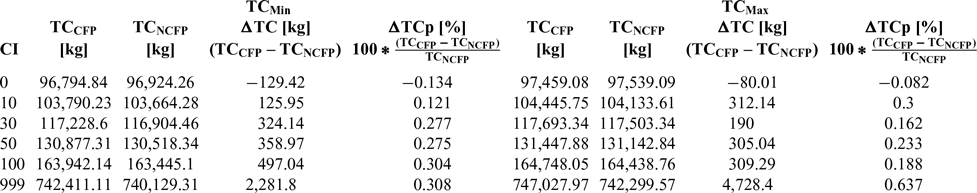
Table 4 Optimisation execution times

The execution times for the optimisation method and the two approaches relative to the invalid flight plans are presented in Table 4. It can be noted that the execution time for the case where the invalid flight plans are corrected (CFP) is more than twice as long as that for the case were they are not corrected (NCFP). This is due to the fact that, when CFP is employed, for each segment, before computing the flight performance for a sub-segment, the altitude–speed combination is validated relative to the flight envelope. If the altitude–speed combination is not valid, the appropriate valid combination must be determined. In both cases, the long execution time can be attributed, in part, to the long flight, the complexity and implementation of the accelerated segment performance calculations, by using an aero-propulsive aircraft performance model, and the large number of sub-segments (integration steps) determined by the lateral flight plan (routing grid) and the vertical flight plan.
The flight plan used as the reference for comparing the performance of the proposed optimisation method was generated based on the SWR40 reference track data. The limitations of the FlightAware flight track data are presented in Section 2.7 (i.e. unknown aircraft configuration, unknown atmospheric conditions encountered by the aircraft, unknown precise times and locations where the flight profile changes occur, etc.). An optimal flight plan (lateral path and altitude–speed flight profile) is specific to an aircraft’s configuration and atmospheric conditions. Therefore, a realistic reference flight plan cannot be constructed by retrieving data from the recorded data.
The reference lateral flight plan was constructed by retaining, from the SWR40 reference track data, a subset of WPTs that best approximate the lateral flight trajectory using the minimum number of orthodromic segments. The selection of the WPTs that define the reference lateral flight plan starts with the initial WPT of the SWR40 reference track. At each step, a new WPT is selected such that it results in the longest orthodromic segment for which the distance from the orthodromic segment to each of the SWR40 reference track data WPTs, situated in-between the two selected WPTs that delimit the orthodromic segment, is smaller than 5n.m. Two more WPTs, denoted as WPTV1 and WPTV2, were added at locations where the vertical flight profile changes occur:
The location of the end of climb phase/beginning of the cruise phase, selected at 300n.m. from the initial WPT; and
The location of the end of cruise phase/beginning of the descent phase, selected at 300n.m. before the final WPT.
If such a location is already among those selected as a lateral flight plan WPT, then there is no need to add it to the reference flight plan.
The lateral component of the reference flight trajectory and the selected significant WPTs, corresponding to the reference flight plan, resulting from the process described above, are presented in Fig. 19. During the accelerated flight simulation, each segment was decomposed into sub-segments (integration steps) with a maximum sea-level length of 50n.m., in which the same laws of variation describe the aircraft performance parameters and evolution. These WPTs are not represented in Fig. 19 because they are specific to the selected flight plan parameters, and they are determined during the accelerated flight performance calculations.

Figure 19. The significant WPTs of the reference lateral flight plan.
The altitude component of the reference vertical flight plan, the initial, final and cruise flight altitudes, as well as the points where the cruise altitude changes occur along the flight track, were all obtained from the SWR40 reference track data (Fig. 20).

Figure 20. Altitude profile for the reference profile.
Given the limitations of the FlightAware flight track data and to obtain a good reference profile, the speed component of the reference flight plan was obtained following an optimisation for the aircraft weight (the same value as used in the proposed method evaluation), atmospheric conditions, reference lateral flight plan and altitude flight plan. The candidate reference plan speed profile is constructed as follows:
A climb and descent at [IAS, MACH] speed schedule pairs; and
It was assumed that the constant-altitude cruise sections are flown at constant speed. Thus, the cruise section contains four constant-speed cruise segments, corresponding to the four constant-altitude cruise segments.
The structure of the speed profile is consistent with the employed aircraft climb/descent speed profiles, and the current navigation paradigm (long cruise segments at constant speed) on busy airways, such as oceanic routes and in congested airspace.
The speed optimisation was performed using a genetic algorithm, similar to the one used in the proposed method (in this case only the speed changes were considered). The speed optimisation was performed five times for each CI value. The population size for the genetic algorithm was selected to be 30, and the number of generations was set at 300. As in the case of the proposed optimisation method, when a profile speed candidate was invalid, the reference speed flight plan optimisation was conducted using two approaches: Corrected Speed Flight Plan (CFP) and Non-Corrected Speed Flight Plan (NCFP).
Table 5 presents the results obtained for the reference flight plan speed optimisation for each of the five CI test runs. The flight plan that yielded the best total cost among the five test runs (marked in the column TCRSmin) was retained as the speed component of the reference vertical flight plan.
Table 5 Reference profile optimisation results

A comparison between the best/worst flight plan optimisation results obtained using the proposed method, and the best reference flight plans is presented in Table 6. The TCRSmin value in Table 6 represents the best total cost (best flight optimisation results) obtained for the reference flight profile, cost index and invalid flight profile correction strategy. The other two columns (‘Best case optimisation results’ and ‘Worst case optimisation results’) represent the best and worst optimisation results obtained using the proposed methodology (minimum and maximum total costs) and the comparison with the best reference profile performance.
Table 6 Flight plan optimisation results: comparison between the best and worst optimisation results versus the best reference flight plan

It can be observed that, for the case where invalid flight plans are corrected (CFP), the best optimisation results (optimal flight plan obtained using the proposed method versus the reference flight plan) gave a reduction of the total cost of between 1.585% and 3.042%. In the worst case, the reduction was found to be between 0.909% and 2.439%.
When invalid flight plans were not corrected (NCFP), the results were found to be better: in the best case, the total cost reduction was between 2.144% and 3.97%, while in the worst case, the total cost reduction was between 1.598% and 3.688%.
For the evaluated test cases, the best results (in terms of both optimisation performance and execution time) were obtained when invalid candidate flight plans were not corrected relative to the aircraft’s flight envelope limitations (NCFP).
4.0 CONCLUSIONS
This paper presents a new method for flight trajectory optimisation, in which the candidate flight trajectories, and thus the optimal flight trajectory, are defined as flight plans decomposed into two elements: a lateral flight plan and a vertical flight plan. The proposed method uses a genetic algorithm to search for the ‘optimum’ flight plan among the set of candidate flight plans that minimises the total cost for the flight. The accelerated flight performance calculations, which construct the flight trajectory resulting from executing a candidate flight plan and compute the flight performance parameters, were conducted using an in-house aircraft performance model that uses the BADA 4.0 APM. The test scenario employed for the evaluation of the proposed method was constructed based on the recorded flight trajectory of a real flight, retrieved from FlightAware, performed with the same aircraft model as used in the calculations.
As expected for optimisations performed using genetic algorithms, for an identical optimisation problem (identical input data), the optimal solution varied from test run to test run. However, for the tests performed in this study, for each of the evaluated test scenarios, the difference between the optimum flight plan total costs obtained for the ten runs was less than 1%. It can be observed that the case where the candidate flight plans are ‘corrected’ (CFP) produces the worst results, in terms of both total cost and total execution time, relative to the case where invalid flight plans are assigned a large penalty total cost (NCFP). The authors believe that, for the cases where the candidate flight plans are ‘corrected’, even though in each new generation all the child flight plans are valid relative to the aircraft’s flight envelope, there is a loss of optimality because, overall, the populations are ‘less diverse’. The increase in execution time is due to the fact that, for each invalid altitude/speed flight plan segment, additional (complex) computations are required to identify the appropriate flight envelope limit combination. For the NCFP approach and the set of CI values considered as test cases, the total cost reduction for the optimal flight plan relative to the best obtained reference flight plan was found to be between 2.144% and 3.97%, while the worst case gave cost reductions between 1.598% and 3.688%. The authors therefore estimate that the longer execution time renders the method more appropriate for flight planning rather that real-time/online optimisation. The longer execution time is due to the large number of flight plans evaluated during the optimisation, the very long flight (5,130.3n.m sea level distance along the orthodromic route), with its large number of integration steps/flight performance calculation steps, and partially due to the flight performance calculations using a dynamic atmosphere model and the aero propulsive/total energy model aircraft performance model.
For any optimal flight plan (local or global), there is a correlation between the lateral and vertical flight plans. Changing/imposing one component of a flight plan could result in a different optimal solution, with a different total cost, and different configuration for the other components of the flight plan. Future work could investigate the performance of a more computationally expensive optimisation approach, where at each step of the genetic algorithm:
The new population is generated using the genetic operations applied on the lateral flight plan (while the vertical flight plan is retained from a parent); and then,
For each member of the new population, a new search (e.g. branch and bound, annealing, etc.) identifies the optimal vertical flight plan.
Another direction of investigation could evaluate the execution time performance of the proposed method when the accelerated flight performance calculations are performed using a simplified aircraft performance model, based on interpolation tables, mainly used in FMS platforms.
ACKNOWLEDGEMENTS
This research was conducted at Laboratory of Research in Active Control, Avionics, and Aeroservoelasticity (LARCASE) in collaboration with CMC Electronics – Esterline and under the auspices of the Green Aviation Research & Development Network (GARDN). The authors thank Mr. Rex Haygate, Mr. Yvan Blondeau, Mr. Dominique Labour, Mr. Oussama Abdul-Baki and Mr. Reza Neshat from CMC Electronics – Esterline, and Mr. Sylvain Cofsky and the Green Aviation Research & Development Network (GARDN) for their support in conducting this research.


