1. INTRODUCTION
With the development of remote sensing technology, Position and Orientation Systems (POSs) are becoming a key motion compensation component, and are capturing growing attention in the high resolution airborne remote sensing field (Mostafa and Hutton, Reference Mostafa and Hutton2001; Zhang et al., Reference Zhang, Qiao, Xing, Yang and Bao2012; Toth, Reference Toth2001; Chen et al., Reference Chen, Ma, Zhang, Liang, Xu and He2011). POSs have a high integration density, and normally consist of Fibre-Optic Gyros (FOG), Inertial Measurement Units (IMU), a Global Navigation Satellite System (GNSS and a Processing Computer System (PCS) to perform Inertial Navigation System (INS)/GNSS data fusion using a Kalman Filter (KF) (Wei et al., Reference Wei, Jin, Yang, Li, Gu and Li2013; Tan et al., Reference Tan, Wang, Jin and Meng2015; Liu et al., Reference Liu, Wei and Jin2017). Consequently, a POS possesses both excellent short-term accuracy provided by the INS solution and consistent long-term accuracy resulting from the GNSS (often the Global Positioning System (GPS)). Moreover, the KF integration, which is based on a linearized dynamic system, improves the overall INS/GPS integrated solution (Grewal, Reference Grewal, Weill and Andrews2007). The model of the INS error dynamics in a POS is linearized to estimate the INS errors. During reliable GPS availability, the KF performs an update step to accurately estimate the INS errors and correct the INS output. However, when GPS signals are unavailable, the update of the POS solution by GPS fails and the navigation output solely depends on the linearized INS error dynamics model to integrate INS measurements. Due to the inaccuracy of integration and the inherent accelerometer bias and gyroscope bias of the IMU, the performance of a POS significantly degrades even during short periods of GPS outages (Hasan et al., Reference Hasan, Samsudin, Ramli and Azmir2011). An optimal real-time algorithm to work around bridging GPS outages is badly needed.
In the last two decades, much work has been done to address GPS outages in INS/GPS integration mode. Ip et al. (Reference Ip, Elsheimy and Mostafa2007) used the Rauch-Tung-Strieble smoothing algorithm for mobile mapping data, which, is a post-processing approach and not applicable to long-term GPS signal loss. Nassar and Schwarz (Reference Nassar and Schwartz2001) proposed a simplified and near real-time model, but assumed that the dominant error is a constant acceleration error, which in reality cannot be satisfied. Zhu and Li (Reference Zhu and Li2016) presented a technique to restrain GPS multi-path errors.
More recently, researchers in the field of multi-sensor fusion and integration have started to shift from conventionally-based approaches toward artificial intelligence-based approaches, aiming at intelligent sensor fusion. In the case of GPS outages, most work has been focused on the combination of Neutral Networks (NN) and KF. For example, Jwo and Huang (Reference Jwo and Huang2004) and Jwo (Reference Jwo and Chen2007) introduced a NN-aided adaptive KF and an extended KF to improve the performance of GPS/INS integrated systems. Wang et al. (Reference Wang, Wang, Sinclair and Watts2006; Reference Wang, Wang, Sinclair and Watts2008) presented a hybrid method to reduce the INS/GPS navigation errors during GPS outages by merging a multi-layered feed-forward back-propagation NN into the KF for GPS/INS integration. Chen and Fang (Reference Chen and Fang2014) put forward a hybrid approach to reduce POS errors during GPS outages by merging NN and an autoregressive model into the KF. Although Chen and Fang proposed the hybrid prediction approach based on an autoregressive model, they applied the autoregressive model solely to express the linear relationship of the time-series measurements using the historical data in their prediction mode; the inherent nonlinearity of time series dynamic data was not well described. Additionally, it is critical to select sufficient data samples of good quality for the neural networks to produce a good performance (Xu et al., Reference Xu, Li, Rizos and Xu2010), which is sometimes too rigorous and limits its practical application. Moreover, a NN-based method has major drawbacks: the existence of a local minimum and the difficulty of choosing the number of hidden units.
Gaussian Process Regression (GPR) as a powerful alternative to neural networks is arousing increasing attention in a wide variety of real-world statistical learning problems (for example, predictions) and model selection procedures (such as nonlinear optimisation problems) (Rasmussen and Williams, Reference Rasmussen and Williams2005; Atia et al., Reference Atia, Noureldin and Korenberg2011). Recently, GPR models have been applied to the learning of inverse dynamic systems (Grimes et al., Reference Grimes, Chalodhorn and Rao2006; Ko et al., Reference Ko, Klein, Fox and Haehnel2007). GPR-based approaches have several significant merits: they are non-parametric; their flexible nonlinear mapping can automatically learn the smoothness and noise levels of the high-dimensional underlying system and they can adequately handle a notion of uncertainty about the underlying process. In addition, the hyper-parameters of a GPR model can be adjusted by maximising the marginal likelihood. The GPR's simplicity and flexibility motivate us to explore its use. Atia et al. (Reference Atia, Noureldin and Korenberg2011) proposed GPR/KF to work around bridging GPS outages in a Micro-Electromechanical Systems (MEMS)/GPS integration. Chen et al. (Reference Chen, Cheng, Wang and Xu2014) merged GPR into a sparse-grid quadrature Kalman filter to address uncertain observation outages. However, as the standard GPR assumes that the input is noise-free, input noise is ignored in both of their methods, which easily leads to poor modelling performance and over-fitting. In addition, all these approaches mentioned above relate INS errors to IMU measurements only at specific time intervals. They do not take into consideration the INS error dependency on the past INS error readings.
In this paper, to maintain the reliable navigation output of a high-precision POS during both short and long GPS outages, we propose a novel hybrid prediction approach based on Noisy Input GPR (NIGPR), which makes NIGPR aid the KF by forecasting the measurement update, rather than replacing the KF. The NIGPR extends GPR to Noisy Input GPR, which is particularly powerful in the case of time-series data with Markovian properties where the output at time t becomes the input at time t+1 by exploiting the inherent structure in input noise data sets. With respect to the INS error dynamics, the current INS errors are related to the previous INS errors, the sum of the gyro and accelerometer measurements from t−1 to t, respectively. Therefore, the NIGPR model is well suited to model the INS error dynamics, predict the measurements as the virtual update of the KF and estimate all the INS errors. This proposed approach was tested using a high-precision fibre POS, and artificial GPS losses with varying lengths were intentionally introduced into the same trajectory to assess the performance of the proposed approach applied to artificial GPS outages with various lengths. Comparing with the two other methods (KF and GPR/KF), the result of the proposed approach was statistically analysed in detail.
The remainder of this paper is organised as follows. Section 2 describes the necessary background of the INS error dynamics, the modelling of INS/GPS integrated systems and Gaussian process regression. The proposed NIGPR/KF hybrid prediction approach and its application in the high-precision POS are presented in detail in Section 3. Subsequently, the performance of the proposed method is evaluated by a real flight experiment in Section 4, and followed by conclusions in Section 5.
2. BACKGROUND THEORY
In this section, we introduce the INS error dynamics, the modelling of INS/GPS integrated systems and then GPR.
2.1. Modelling the INS/GPS Integrated System
Owing to the integrations implicit within the calculations, the INS output drifts over time, which causes bias errors of both accelerometer and gyroscope measurements to be accumulated at the output (Chatfield (Reference Chatfield1997)). To compensate INS errors, observation measurements of superior accuracy are periodically utilised. Observation measurements may be related to some of the INS error states. For a POS, KF observation measurements consist of the difference between the GPS and INS position and velocity information. The KF procedure is divided into two stages: prediction, which solely relies on past information and the INS error dynamic model, and update, which incorporates the information obtained using the GPS solution. When there are no GPS outages, the KF utilises this information to estimate and update the errors in the state vector. When the GPS signal is lost and outages occur, only the prediction stage of the KF algorithm is used to progress the INS error dynamics model and update the state estimate. Thus, the KF requires an INS error dynamics model, a dynamic model of both INS and GPS errors and a priori information about the covariance of the data provided by both models. In the following, their details will be introduced.
Before introducing the INS error dynamics, n denotes the local level navigation frame, b the INS body frame, i the inertial frame and e the Earth frame. The states of the KF for a POS are composed of the position, velocity, and attitude equations and the error equations of the gyroscopes and the accelerometers.
The INS error dynamics model can be expressed by following equations, see Groves (Reference Groves2013).
 $$\eqalign{ \dot \phi &= \phi \times \omega _{in}^n + \delta \omega _{in}^n - C_b^n \varepsilon \cr \delta \dot v_n &= f_n \times \phi - \delta [(\omega _{ie}^n + \omega _{in}^n ) \times v_n] + C_b^n \nabla \cr \delta \dot r_n &= \delta v_n + \rho \times \delta r_n \cr \dot \varepsilon &= 0 \cr \dot \nabla &= 0}$$
where,  $\phi =[\phi _{E} ,\phi _{N} ,\phi _{U} ]^{T}$ represents the misalignment angles at the current moment.
  $v_{n} =[v_{E}^{n} ,v_{N}^{n} ,v_{U}^{n} ]^{T}$ and
  $\delta v_{n} =[\delta v_{E}^{n} ,\delta v_{N}^{n} ,\delta v_{U}^{n} ]^{T}$ denotes the current velocity and its error with respect to the navigation frame, respectively.
  $r_{n} =[L,\lambda ,h]^{T}$ and
  $\delta r_{n} =[\delta L,\delta \lambda ,\delta h]^{T}$ represents the current position and its error with respect to the navigation frame, respectively.
  $f_{n} =[f_{E} ,f_{N} ,f_{U} ]^{T}$ denotes the specific force vector with respect to the navigation frame,
  $\varepsilon =[\varepsilon _{x} ,\varepsilon _{y} ,\varepsilon _{z} ]^{T}$ represents the gyro bias and
  $\nabla =[\nabla _{x} ,\nabla _{y} ,\nabla _{z} ]^{T}$ represents the accelerometer bias. f n is the projection of the accelerometer measurements in the navigation frame.
  $\omega _{ie}^{n} =[0,\Omega _{N} ,\Omega _{U} ]^{T}$ represents the local Earth rotation rate vector of the e-frame with respect to the i-frame in the n-frame, with
  $\Omega _{N} =\omega _{e} \cos L,\Omega _{U} =\omega _{e} \sin L$ and ωe is the Earth rotation rate.
  $\omega _{in}^{n} =[-\dot{L},\dot{\lambda}\cos L+\Omega _{N} ,\dot{\lambda} \sin L+\Omega _{U} ]$ with
  $\dot{L} =v_{N}^{n} /R_{M} \dot{\lambda} =v_{E}^{n} \sec L/R_{N} $,
  $R_{M} =R_{e} (1-2e+3e\sin ^{2}L)$,
  $R_{N} =R_{e} (1+e\sin ^{2}L)$, R e is the semi-major axis of the ellipsoid and e is the eccentricity,
  $\rho =[-\dot{L},\dot{\lambda} \cos L,-\dot{\lambda} \sin L]^{T}$ and the symbol
  $^{\prime}\times ^{\prime}$ denotes the cross product of the vector. The subscript E, N and U denote the east, north and up components in the n-frame, and the subscript x, y and z denote the right, front and up components in the b-frame.
  $C_{b}^{n}$ is given by
 $$C_b^n = \left[\matrix{ {C_{11}} & { - \cos \theta \sin \psi } & {C_{13}} \cr {C_{21}} & {\cos \theta \cos \psi } & {C_{23}} \cr { - \sin \gamma \cos \theta } & {\sin \theta } & {\cos \gamma \cos \theta }} \right]$$
where C 11 = cos γ cos ψ – sin γ sin θ sin ψ, C 21 = cos γ sin ψ + sin γ sin θ cos ψ, C 13 = sin γ cos ψ + cos γ sin θ sin ψ and C 23 = sin γ sin ψ – cos γ sin θ cos ψ . ψ, θ and γ represent the heading, pitch and roll angles in the n-frame, respectively.
Since the state model shown above is linear, which can be simplified using a state-space representation with system equation, depicted as Equation (2)
 $$x_{k+1} =F_k x_k +G_k w_k$$
where,  $x_{k} =[\phi ^{T},\delta v_{n} ^{T},\delta r_{n} ^{T},\varepsilon ^{T},\nabla^{T}]$, w k is the Gaussian white noise process of zero mean and covariance matrix Q k, which is
  $G_{k} w_{k} G_{k}^{T} $. The matrices F k and G k are as follows
 $$F_k =\left[ \matrix{{F_{11} } & {F_{12} } & {F_{13} } & {C_b^n } & {0_{3\times 3}} \cr {F_{21} } & {F_{22} } & {F_{23} } & {0_{3\times 3} } & {C_b^n } \cr {0_{3\times 3} } & {I_{3\times 3} } & {F_{33} } & {0_{3\times 3} } & {0_{3\times 3} } \cr {0_{3\times 3} } & {0_{3\times 3} } & {0_{3\times 3} } & {0_{3\times 3} } & {0_{3\times 3} } \cr {0_{3\times 3} } & {0_{3\times 3} } & {0_{3\times 3} } & {0_{3\times 3} } & {0_{3\times 3}}} \right]$$
 $$F_{11} =\left[ \matrix{ 0 & {\Omega_U +\dot{\lambda} \sin L} & {-(\Omega_N +\dot{\lambda} \cos L)} \cr {-(\Omega_U +\dot{\lambda}\sin L)} & 0 & {-\dot{L} } \cr {\Omega_N +\dot{\lambda}\cos L} & {\dot{L}} & 0} \right]$$
 $$F_{12} =\left[ \matrix{ 0 & {-1/(R_M +h)} & 0 \cr {1/(R_N +h)} & 0 & 0 \cr {\tan L/(R_N +h)} & 0 & 0} \right]$$
 $$F_{13} =\left[ \matrix{ 0 & 0 & 0 \cr {-\Omega_U } & 0 & 0 \cr {\Omega_N +\dot{\lambda}\sec L} & 0 & 0} \right]$$
 $$F_{21} =\left[ \matrix{ 0 & {-f_U } & {f_N } \cr {f_U } & 0 & {-f_E } \cr {-f_N L} & {f_E } & 0} \right]$$
 $$F_{22} =\left[ \matrix{ {-\dot{L}\tan L-\dot{h} } & {2\Omega_U +\dot{\lambda} \sin L} & {-2\Omega_N -\dot{\lambda} \cos L} \cr {-2(\Omega_U +\dot{\lambda} \sin L)} & {-\dot{h}} & {-\dot{L}} \cr {2(\Omega_N +\dot{\lambda} \cos L)} & {2\dot{L}} & 0} \right]$$
 $$F_{23} =\left[ \matrix{ {2(\Omega_N v_N +\Omega_U v_U )+\dot{\lambda}v_N \sec L} & 0 & 0 \cr {-2(\Omega_N +\dot{\lambda}\sec L)v_E } & 0 & 0 \cr {-2\Omega_U v_E } & 0 & 0} \right]$$
 $$F_{33} =\left[ \matrix{{2(\Omega_N v_N +\Omega_U v_U )+\dot{\lambda} v_N \sec L} & {\dot{\lambda}\sin L} & {\dot{\lambda} \cos L} \cr {-\dot{\lambda}\sin L} & 0 & {\dot{L} } \cr {-\dot{\lambda}\cos L} & {{-\dot{L}}} & 0} \right]$$
 $$G_k =\left[ \matrix{ {C_b^n } & {0_{3\times 3} } \cr {0_{3\times 3} } & {C_b^n } \cr {0_{3\times 3} } & {0_{3\times 3} } \cr {0_{3\times 3} } & {0_{3\times 3} } \cr {0_{3\times 3} } & {0_{3\times 3}}} \right]$$
The measurement z k of the KF is obtained from the difference of velocity and position resulting from the INS solution and GPS solution, respectively.
 $$z_k =[(\delta v_n')^T,(\delta r_n' )^T]$$
 where  $(\delta v_{n}')^{T}=v_{n} -v_{GPS} $,
  $(\delta r_{n}')^{T}=r_{n} -r_{GPS}$,
  $v_{GPS} =[v_{GPS}^{E} ,v_{GPS}^{N} ,v_{GPS}^{U} ]^{T}$,
  $r_{GPS} = [r_{GPS}^{E},\break r_{GPS}^{N} ,r_{GPS}^{U} ]^{T}$ and v GPS and r GPS represent the velocity and position vector from the GPS, respectively. Hence, the measurement equation of the POS can be given by
 $$z_{k+1} =H_{k+1} x_{k+1} +\nu _{k+1}$$
where  $H_{k+1} =[H_{V} ,H_{P} ]^{T}$,
  $H_{V} =[0_{3\ast 3} ,\hbox{diag}(1,1,1),0_{3\ast 9}]$,
  $H_{P} =[0_{3\ast 6} ,\hbox{diag}(1,1,1),0_{3\ast 6}]$ and ν is the measurement noise, which is a zero-mean Gaussian white noise vector and covariance matrix R k+1. Up to now the integrated system can be described by the state space Equation (2) and measurement Equation (4).
When GPS outages occur, the KF is not updated by the GPS. How to model the inherent nonlinearity of the INS error dynamics is further discussed in detail in Section 3.
2.2. Gaussian Process Regression
A GPR is often thought of as a Gaussian distribution over functions (Roberts et al., Reference Roberts, Osborne, Ebden, Reece, Gibson and Aigrain2012). It can be viewed as the generalisation of a Gaussian distribution over a finite vector space to a function space of infinite dimensions. Just as both a mean and covariance matrix can fully specify a Gaussian distribution, a Gaussian Process (GP) is fully described by its mean and covariance function K. Although functions are infinitely dimensional, GPs are used to preform prediction, or inference of function values at a finite set of prediction points from the observed data. Assuming that the pair-wise training data set  $D=\lcub {\lpar {x_{1} ,y_{1}} \rpar ,\lpar {x_{2} ,y_{2} } \rpar ,\lpar {x_{3} ,y_{3}} \rpar ...\lpar {x_{n} ,y_{n} } \rpar } \rcub $, is formulated by the following noisy process
 $$y_i =f(x_i )+\delta _{out}^2$$
where the variance  $\delta _{out}^{2}$ is the Gaussian white noise with zero mean. x i and y i form pair-wise measurement vectors X in and Y out, respectively.
For GPs, the covariance forms the beating heart of Gaussian process inference. The covariance kernel function, k(x i, x j) provides the covariance element between any two arbitrary sample points x i and x j. Many kernels have been designed to capture various properties of the modelled phenomenon including smoothness and stationarity. They are constructed to guarantee that any matrix obtained from them is a positive semi-definite covariance matrix, irrespective of the choice of inputs. Kernels can be combined to form new kernels. Each kernel has a set of hyper-parameters which control the magnitude of the covariance eigenvalues and the degree of correlation between the outputs. Here, we define the covariance matrix K(X in, X in), and for details about the kernel function, please see Rasmussen et al. (Reference Rasmussen and Williams2005).
Consequently, the observed output can be modelled by the Gaussian distribution, as per the following formulation
 $$P(Y_{out} )=N(\mu ,\hbox{K}(X_{in} ,X_{in} )+\delta _{out}^2 )$$
where μ is the mean function.
Thus, the Gaussian process posterior distribution of Y* at some test datum X* outside our observations is evaluated. The posterior mean and variance can be given by Equation (7)
 $$P(Y^\ast )=N(\mu ^\ast ,C^\ast )$$
where  $\mu ^{\ast} =\mu (X^{\ast} )+\hbox{K}(X^{\ast} ,X_{in} )[\hbox{K}(X_{in} ,X_{in} )+\delta_{out}^{2} ]^{-1}(Y_{out} -\mu ), C^{\ast} =\hbox{K}(X^{\ast} ,X^{\ast} )-\hbox{K}(X^{\ast} ,\break X_{in} )[\hbox{K}(X_{in} ,X_{in} )+\delta _{out}^{2} ]^{-1}\hbox{K}(X_{in} ,X^{\ast} )$ and where
  $[\hbox{K}(X_{in} ,X_{in} )+\delta _{out}^{2} ]^{-1}$ is precomputed in the prediction mode.
3. DESIGN OF NIGPR AND KF HYBRID PREDICTOR FOR BRIDGING GPS OUTAGES IN POS
In this section, modelling the NIGPR of the INS error dynamics is introduced, then we train the NIGPR model of INS error dynamics, and further predict the observation measurement based on the trained model when GPS outages occur.
3.1. Modelling NIGPR of the INS error dynamics
A NIGPR for the motion model learns the position error and velocity error from one time step to the next. This is similar to the modelling of the INS error dynamics. Therefore, the NIGPR model can be used to model INS error dynamics by learning the function f based on the collected data set consisting of the sum of sequential gyro and accelerometer measurements from time k−1 to k and the previous INS errors of position and velocity. In this paper, given the previous deviation errors with the control input of gyroscopes and accelerometers measurements, the NIGPR model has to predict the next position and velocity errors using the difference between the position and velocity from INS and GPS during reliable GPS availability. It can be viewed as a set of time series measurements of uniform frequency and can be written as
 $$x_k =f(x_{k-1} ,u_k )+\delta _{out}^2$$
where k is the time mark and f is a function which describes the error dynamics of the INS during GPS signal outages, u k is also used to serve the input of the function f, and it is made up of the sum of the gyroscope and accelerometer measurements at the rate of 200 Hz from k−1 to k, which has an important effect on the errors of INS. x k is redefined by observation measurement vector  $Z_{k} =\left[ \matrix{{V_{k}^{INS} -V_{k}^{GPS} } \cr {P_{k}^{INS} -P_{k}^{GPS} } } \right]$, which can be rewritten as follows
 $$x_k =Z_k =\left[ \matrix{ {V_k +\delta V_k^{INS} +n_k^{INS} -(V_k +n_k^{GPS} )} \cr {P_k +\delta P_k^{INS} +m_k^{INS} -(P_k +m_k^{GPS} )} } \right]=\left[ \matrix{ {\delta V_k^{INS} +ev_k } \cr {\delta P_k^{INS} +ep_k } } \right]$$
where  $P_{k}^{INS}$ and
  $V_{k}^{INS}$ denote the position and velocity of the INS, which are calculated through integrating the measurements of gyroscopes and accelerometers after online error compensation at time k,
  $P_{k}^{GPS}$ and
  $V_{k}^{GPS}$ denote the position and velocity of GPS measurements at time k, P k and V k denote the real position and velocity of the body at time
  $k. \delta P_{k}^{INS}$ and
  $\delta V_{k}^{INS}$ denote the stochastic position and velocity errors of the INS, deviating from the real values at time k. Its model is built by the function f in Equation (8).
  $ev_{k} =n_{k}^{INS} -n_{k}^{GPS}$ and
  $ep_{k} =m_{k}^{INS} -m_{k}^{GPS}$ denote the measurement noise from the position and velocity at time k, respectively.
It is widely acknowledged that inertial errors are the main source of the observation measurement, which results from integrating the angular velocity  $\omega _{ib}^{b}$ and the specific force
  $f_{ib}^{b}$ measured from gyros and accelerometers of the body frame with respect to the inertial frame. Therefore, they can be selected as the input of the NIGPR model. In addition, the observation measurements have such strong Markovian properties and nonlinear relationships that the previous observation Z k−1 can also be selected as the input of the NIGPR. The current observation measurement Z k is viewed as the output of the NIGPR. Thus far, the NIGPR model can be used to model the INS error dynamics.
Just as with a standard GPR, NIGPR is also fully described by its mean and covariance functions. The NIGPR can be modelled as follows
 $$Z_{in} = z_{in} +\delta _{in}^2 ,Z_{out} =z_{out} +\delta _{out}^2$$
 $$Z_{out} = f(Z_{in} -\delta _{in}^2 ,\theta )+\delta _{out}^2$$
 $$f \sim N\left(\mu ,\sum \right)$$
where the target observation vector Z out is within the area of Z 1 to Z k, which has six dimensions, and the input observation vector Z in is within the area of Z 0 to Z k−1 and corresponding measurements resulting from the gyroscopes and accelerometers have 12 dimensions. μ is the GPR a priori mean, ∑ is the GPR covariance matrix, and θ is the hyper-parameter which contains the GPR kernel function hyper-parameter, the output Gaussian noise variance  $\delta _{out}^{2}$ and the input Gaussian noise variance
  $\delta _{in}^{2}$.
However, the posterior distribution of a NIGPR model based on the above equation is intractable; it can be approximately solved by the Taylor expansion about the input Z in. For computational convenience, the Taylor expansion is up to a first term with the linear model for the noisy input as follows
 $$Z_{out} =f(Z_{in} )+(\delta _{in}^2 )^T\partial _{\overline f } +\delta_{out}^2$$
As a result, the observed output can be modelled by the Gaussian distribution, as formulated by Equation (14).
 $$P(Z_{out} \vert f)=N(f\!, \hbox{K}+(\delta _{in}^2 )^T\partial _{\overline f } +\delta_{out}^2 )$$
The Gaussian a priori process is represented by Equation (15).
 $$P(f\vert Z_{in} )=N(0,\hbox{K})$$
where K = K(Zin, Zin) is a covariance matrix computed using a given covariance kernel function. In this paper, the widely prevalent Gaussian kernel is the squared exponential kernel function given by  $k(Z_{i} ,Z_{j})=\sigma _{f}^{2} \exp (-0.5(Z_{i} -Z_{j} )^{T}S(Z_{i} -Z_{j} ))$, in which S controls the input scale of the kernel function.
As a result, the NIGPR learns to predict the next state, conditioned on the previous state and control input.
3.2. Training the hybrid predictor
When a GPS solution is obtained periodically, the GPS information can be used to update the observation measurement Z k using the difference between the GPS and INS positions and the velocities as in Equation (9), thus, the proposed NIGPR/KF hybrid predictor system operates in the training mode. In order to learn the NIGPR model, the obtained Z k can be selected as the target output of the NIGPR model, the corresponding input vector is provided by the previous Z k−1 and the sum of gyroscope and accelerometer measurements from time k−1 to k, respectively. These hyper-parameters of the NIGPR model (input noise, input scale and output noise) can be learned by maximising the negative log likelihood of the pair-wise training data set using the common gradient optimisation method as in Equations (16)-(18). Equation (16) describes the object function to be trained, and in order to optimise it, its negative log likelihood should be calculated using Equation (17). In Equation (18), we optimise its negative log likelihood to maximise the hyper-parameters using the Broyden–Fletcher–Goldfarb–Shanno (BFGS) method (Mokhtari and Ribeiro, Reference Mokhtari and Ribeiro2014). Figure 1 shows a block diagram representation of the common KF update and training mode of operation for the hybrid predictor system during GPS availability.
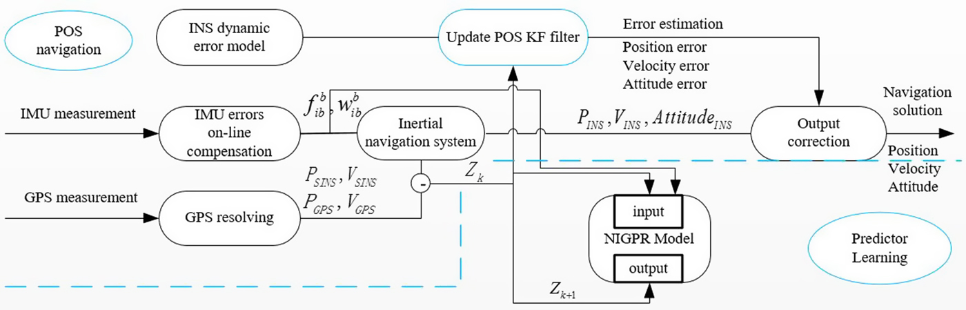
Figure 1. Block diagram of NIGPR/KF hybrid predictor during GPS availability.
 $$L_{NIGP} (Z_{out} \vert Z_{in} ,\theta )\sim N(Z_{out} \vert m(Z_{in} ),M)$$
 $$-\log L_{NIGP} (Z_{out} \vert Z_{in} ,\theta )={d \over 2}\log 2\pi +{1 \over 2}\log \vert M\vert +{1 \over 2}(m(Z_{in} )-Z_{out})^TM^{-1}(m(Z_{in} )-Z_{out})$$
 $$\theta _{\max} =\arg \max \lcub {-\hbox{log}\, L_{NIGP} (Z_{out} \vert Z_{in},\theta )} \rcub $$
where m denotes the mean,  $M=K+\delta _{out}^{2} +\overline \sum (Z_{in} )$.
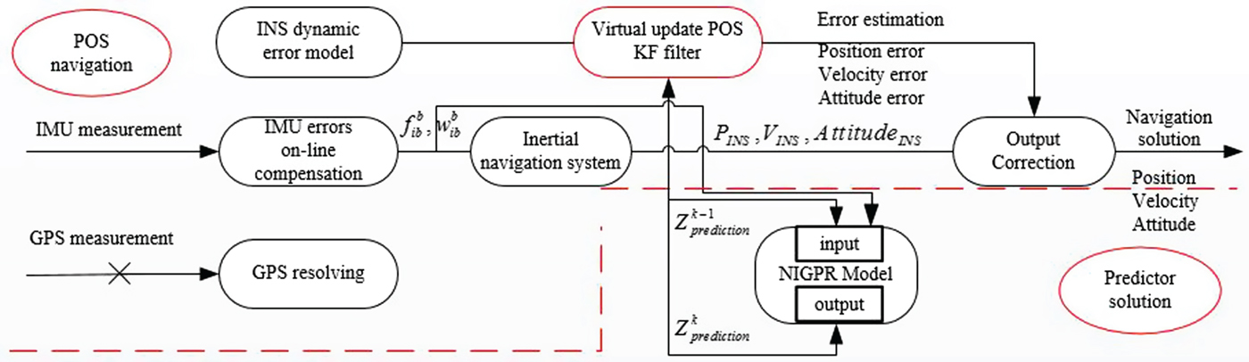
When GPS outages occur, a practical KF update step will be not be periodically performed, and the POS will operate the prediction mode using the learned model.  $Z_{prediction}^{k-1} $ and the sum of gyroscopes and accelerometers measurements from time k−1 to k respectively, are used as the input for the predictor system, denoted by
  $Z_{in}^{k-1}$. Figure 2 shows a block diagram representation of the virtual update mode of operation for the hybrid predictor system during GPS outages.

Figure 2. Block diagram of NIGPR/KF hybrid predictor during GPS outages.
The above analysis shows the posteriori distribution over  $Z_{prediction}^{k} $ is made up of the mean and variance at a previous data point
  $Z_{in}^{k-1} $. Combining the probability distribution of Equations (14) and (15), the predicted output for unseen input vector
  $Z_{in}^{k-1} $ serves a Gaussian probability distribution whose mean and variance are obtained from Equations (20) and (21). Therefore, the POS KF then performs a virtual update step to estimate all INS errors with the prediction mean
  $K^{\ast} M^{-1}Z_{out}$ and prediction variance
  $R_{k+1} ={\mathop \delta \limits^{\wedge}}^{2}_{Z_{in}^{k-1}}$ and produces a correct INS output.
 $$\left[ \matrix{ {Z_{prediction}^k } \cr {Z_{out} }} \right]\sim N\left( {\left[ \matrix{ 0 \cr 0 } \right],\left[ \matrix{ N & {K^\ast } \cr {(K^\ast )^T} & M } \right]} \right)$$
 $$\mu _{Z_{in}^{k-1} } =K^\ast M^{-1}Z_{out}$$
 $${\mathop \delta \limits^\wedge}_{Z_{in}^{k-1}}^{2} =N-K^{\ast} M^{-1}(K^{\ast})^{T}$$
where  $K^{\ast} =K(Z_{in}^{k-1} ,Z_{in} )$,
  $(K^{\ast} )^{T}=K(Z_{in} ,Z_{in}^{k-1})$,
  $K^{\ast \ast }=K(Z_{in}^{k-1} ,Z_{in}^{k-1} )$ and
  $N=K^{\ast \ast}+\delta _{out}^{2} +\overline \sum (Z_{in}^{k-1} )$.
4. EXPERIMENTAL RESULTS AND ANALYSIS
In order to evaluate the performance of the proposed NIGPR/KF hybrid prediction approach, a real flight experiment combining POS and a Synthetic Aperture Radar (SAR) was carried out in 2015, in Shan Xi Province, China. Figure 3 shows the airplane in the test. The flight data including GPS, IMU and navigation data was all received, thus the post-processing solution from POS in this case serves as the baseline for testing the POS accuracy during the artificial GPS outages. The flight data was collected by Beihang University, Beijing, China.

Figure 3. The airplane in the flight test.
4.1. Hardware configuration
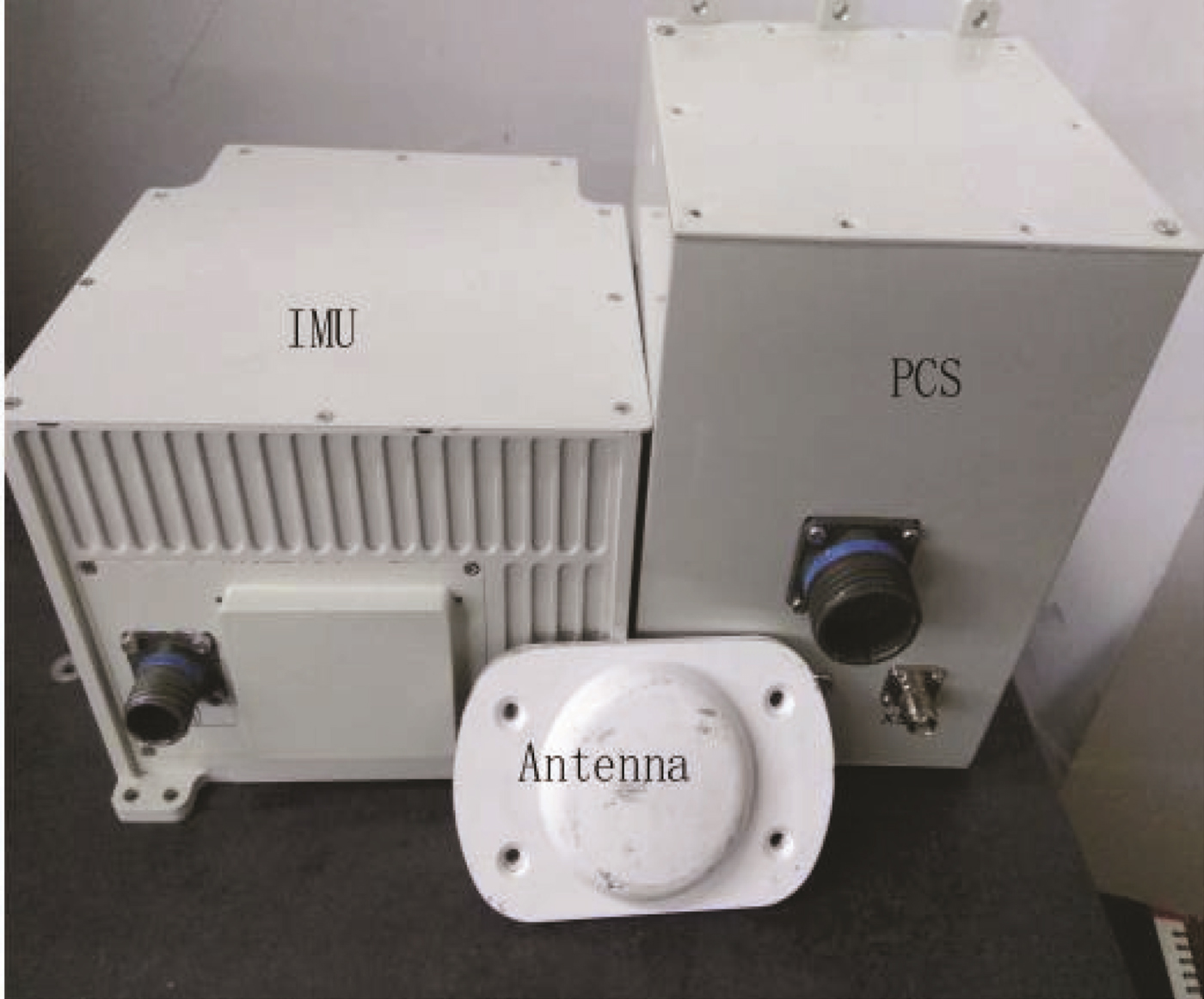
The proposed approach used the newest high-precision FOG POS designed by the POS Research Group at Beihang University. The FOG POS consists of a FOG IMU and PCS on board as shown in Figure 4. The ground base station equipment with Real-Time Kinematic (RTK) transmitting antenna, GPS base antenna and Novatel DL-V3 GPS base receiver was erected on a permanent position, as shown in Figure 5. The parameters of the TX-G120C POS are listed in Table 1. The PCS is installed on the test airplane, and the IMU is mounted on the back of the SAR.

Figure 4. POS on board in the flight test.

Figure 5. Base station equipment of POS on the ground.
Table 1. Specifications of TX-G120C POS.

4.2. Experiment scheme arrangement
The effectiveness of the proposed NIGPR/KF hybrid technique is examined by the POS data obtained from the real flight test. The whole flight trajectory is shown in Figure 6. The POS worked well, and no GPS outages occurred. The increased accuracy of NIGPR/KF comes with increased computational complexity and the need for training data that covers the complete operational space of the dynamical system. To keep accuracy high while reducing computational complexity, the training data for the NIGPR is obtained from a typical run of the airplane.
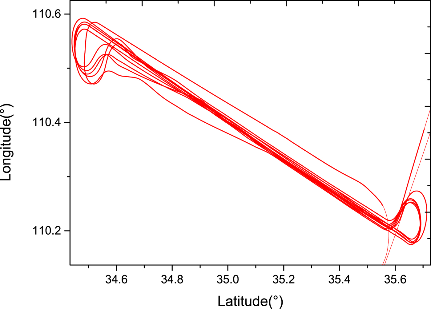
Figure 6. The real flight trajectory in the experiment.
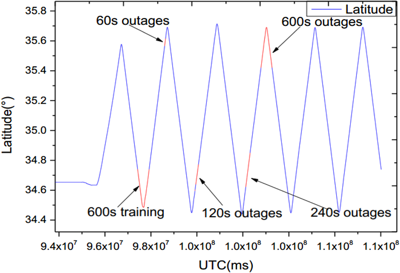
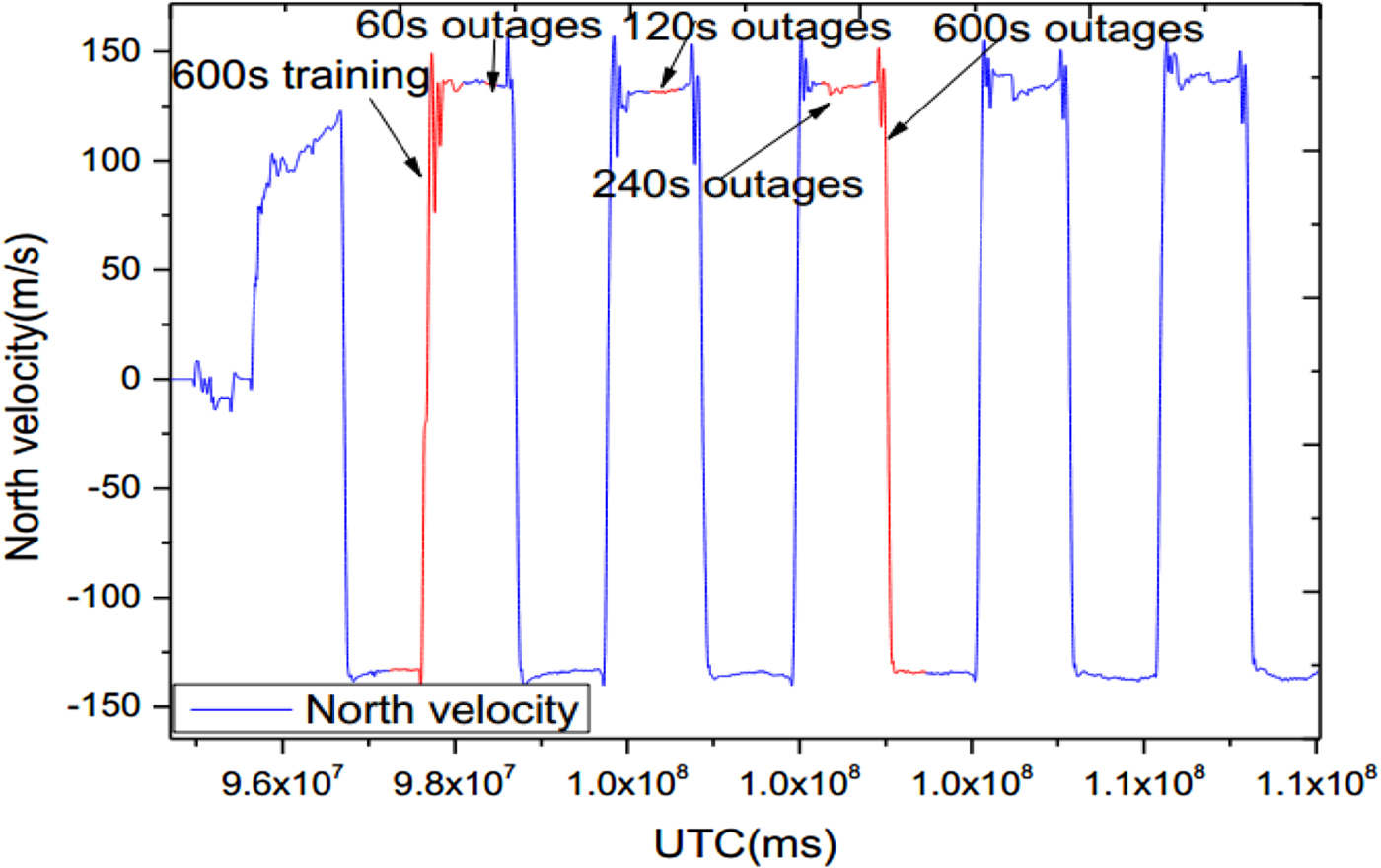
In this experiment, the training data only covered a small starting envelope around the real trajectory. It included two straight sections and two turns, which was used to model the NIGPR of the INS error dynamics. Then four various artificial GPS outages (60 s, 120 s, 240 s and 600 s) were intentionally introduced during post-processing. Table 2 provides the start and stop timings for the training NIGPR model and the four various GPS outages. Figure 7 and 8 show the latitude locations and the north velocity variations of five GPS time sections for training and four outages, respectively.

Figure 7. Latitude varying over artificial GPS outage periods.

Figure 8. North velocity varying over artificial GPS outages.
Table 2. The start and stop times for training the NIGPR model and GPS outages.
4.3. Data processing and results analysis
A real-time POS processing software package developed by the POS Research Group of Beihang University was used to provide the navigation by integrating INS measurements and fusing real-time sequential INS and GPS data. The high precision properties of POS navigation are presented in Table 1, and serves as the baseline data to evaluate the effectiveness of the proposed hybrid prediction approach. In this paper, we consider the cases of GPS outages with various lengths (60 s, 120 s, 240 s and 600 s), and fuse the INS/GPS data using three different solutions, which are a 15 state KF solution, the GPR/KF solution and the proposed hybrid prediction solution. The results of the solutions are compared in the case of the same trajectory and identical GPS outages. In addition, to simulate the real-time processing of the POS, we developed an INS/GPS integration software package based on the NIGPR model using Microsoft Visual Studio 2010. When a case of GPS outage occurs, the learned NIGPR model works in a prediction mode, and predicts the observation measurement.
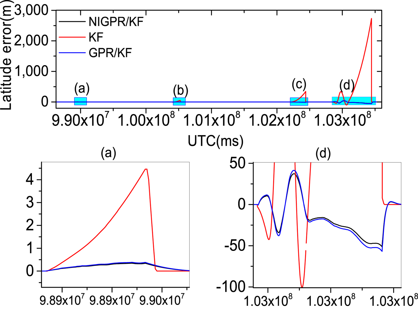
Figures 9–14 show the position and velocity error curves of the three solutions in cases of GPS outages with various lengths (60 s, 120 s, 240 s and 600 s). Since attitude error is barely influenced by GPS outages in a high-precision POS, the attitude errors are not taken into consideration in this paper. The errors of the KF solution greatly increase during GPS outages, where the stand-alone INS output errors growth rate is directly proportional to the length of outage. Since there is no GPS information available for updating the INS position and velocity components, INS errors accumulate with time and cause a significant degradation in the POS accuracy over these cases of GPS outages.

Figure 9. The top row is latitude error curves; (a), (b), (c) and (d) represent the 60 s, 120 s, 240 s and 600 s GPS outages, respectively; in the second row, the panels (a) and (d) are the enlarged views of latitude error corresponding to the GPS outages of 60 s and 600 s, respectively

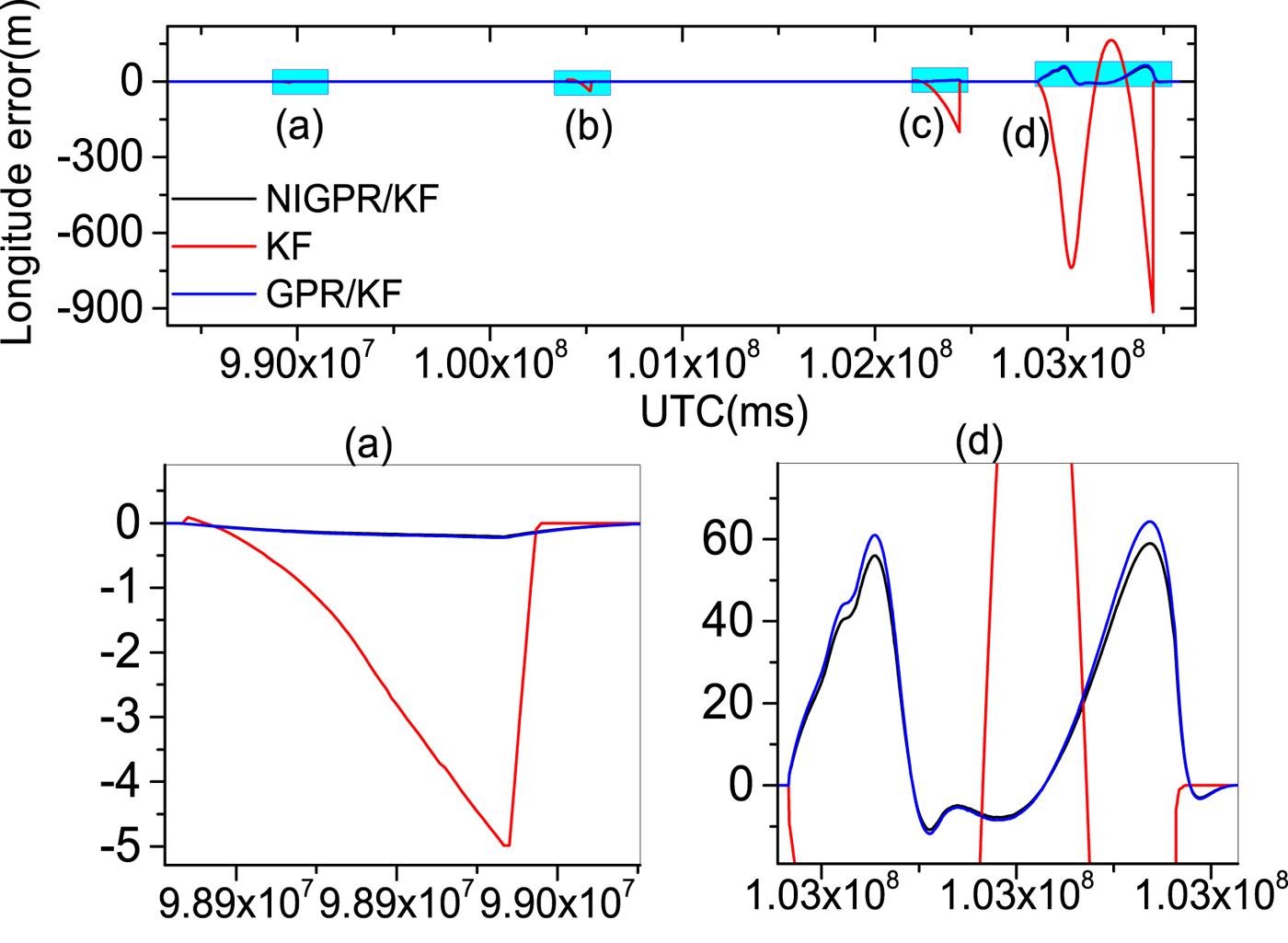
Figure 10. The top row is longitude error curves; (a), (b), (c) and (d) represent the 60 s, 120 s, 240s and 600 s GPS outages, respectively; in the second row, the panels (a) and (d) are the enlarged views of longitude error corresponding to the GPS outages of 60 s and 600 s, respectively

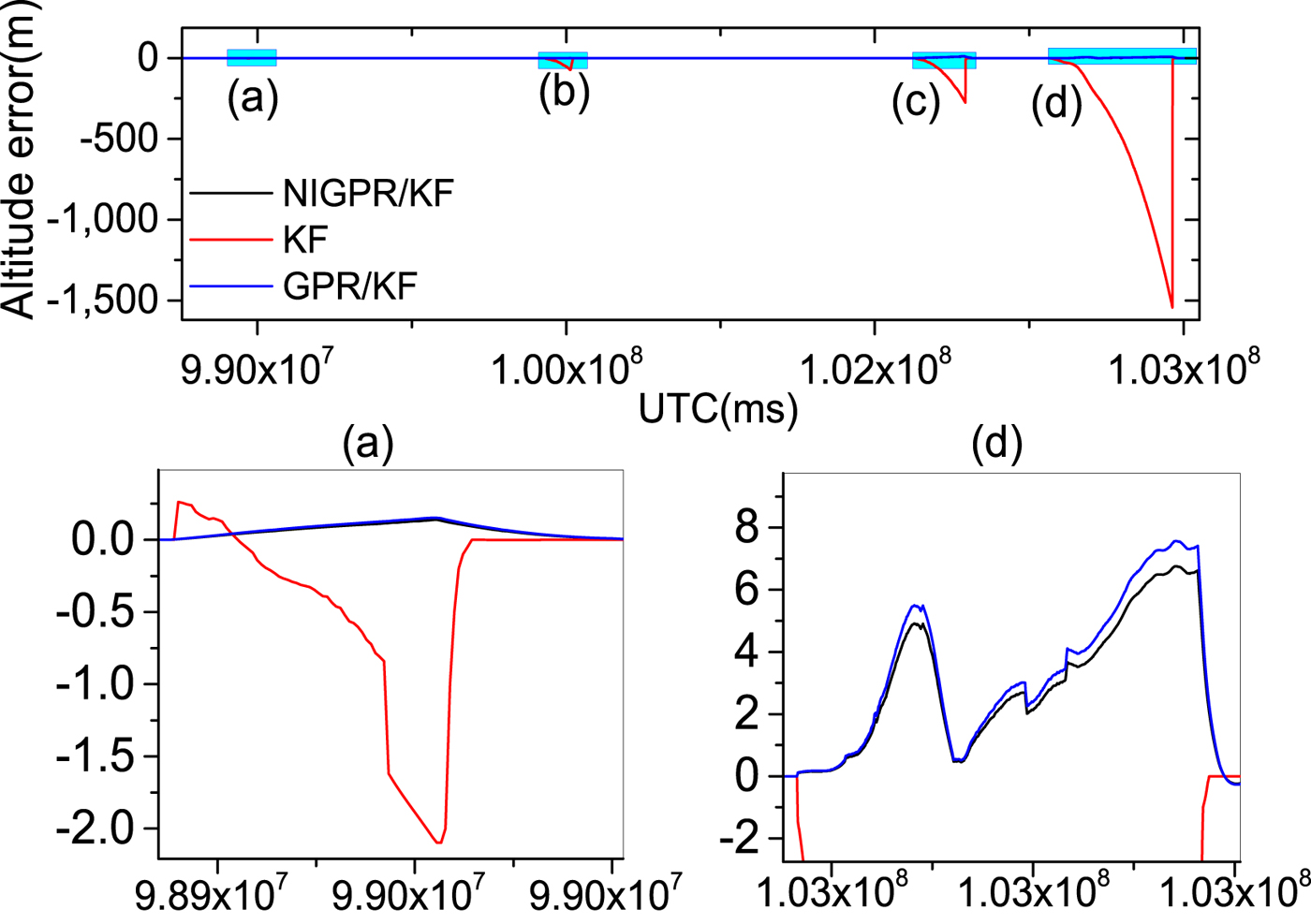
Figure 11. The top row is altitude error curves; (a), (b), (c) and (d) represent the 60 s, 120 s, 240 s and 600 s GPS outages, respectively; in the second row, the panels (a) and (d) are the enlarged views of altitude error corresponding to the GPS outages of 60 s and 600 s, respectively.
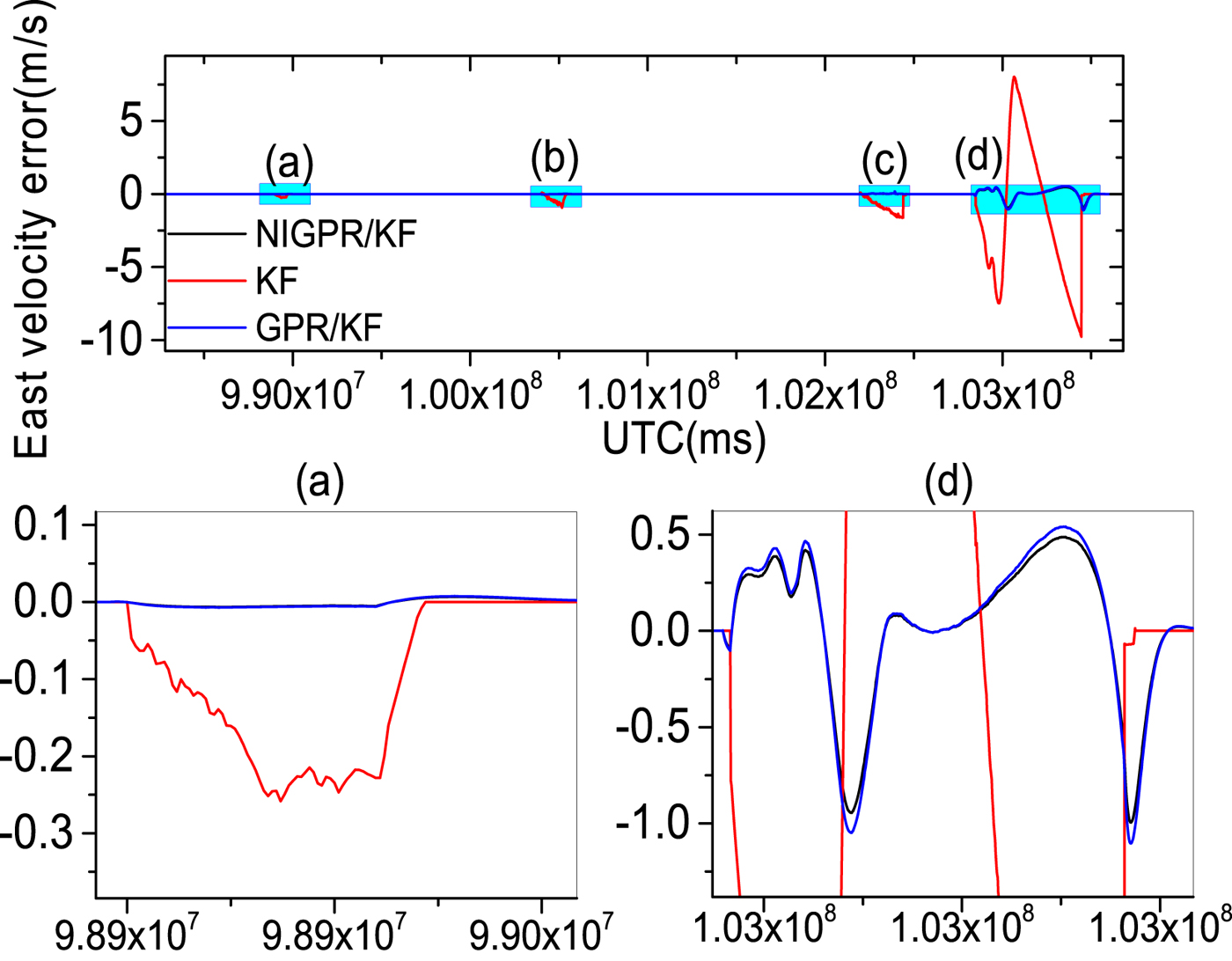
Figure 12. The top row is east velocity error curves; (a), (b), (c) and (d) represent the 60 s, 120 s, 240 s and 600 s GPS outages, respectively; in the second row, the panels (a) and (d) are the enlarged views of east velocity error corresponding to the GPS outages of 60 s and 600 s, respectively.
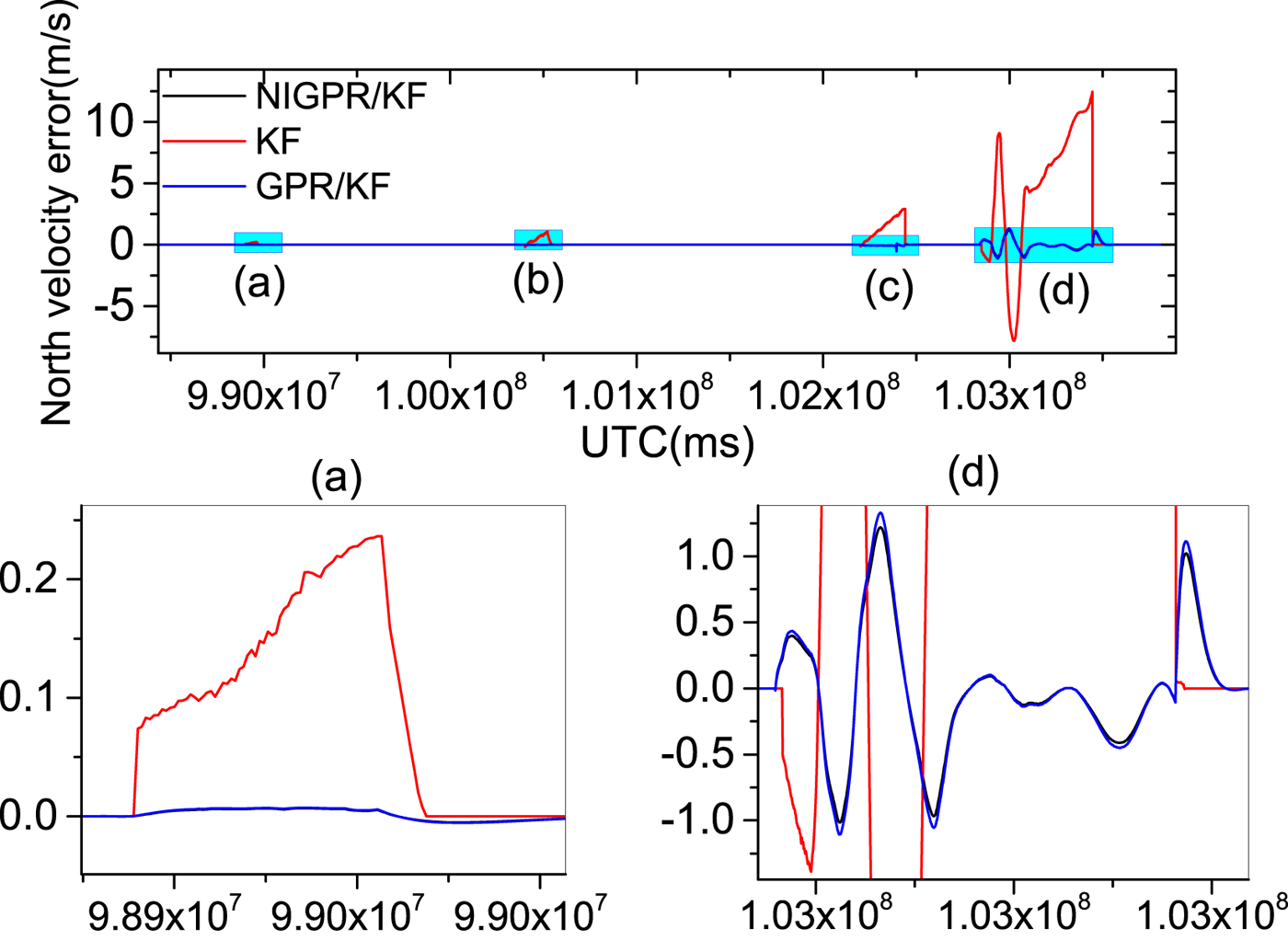
Figure 13. The top row is north velocity error curves; (a), (b), (c) and (d) represent the 60 s, 120 s, 240 s and 600 s GPS outages, respectively; in the second row, the panels (a) and (d) are the enlarged views of north velocity error corresponding to the GPS outages of 60 s and 600 s, respectively.

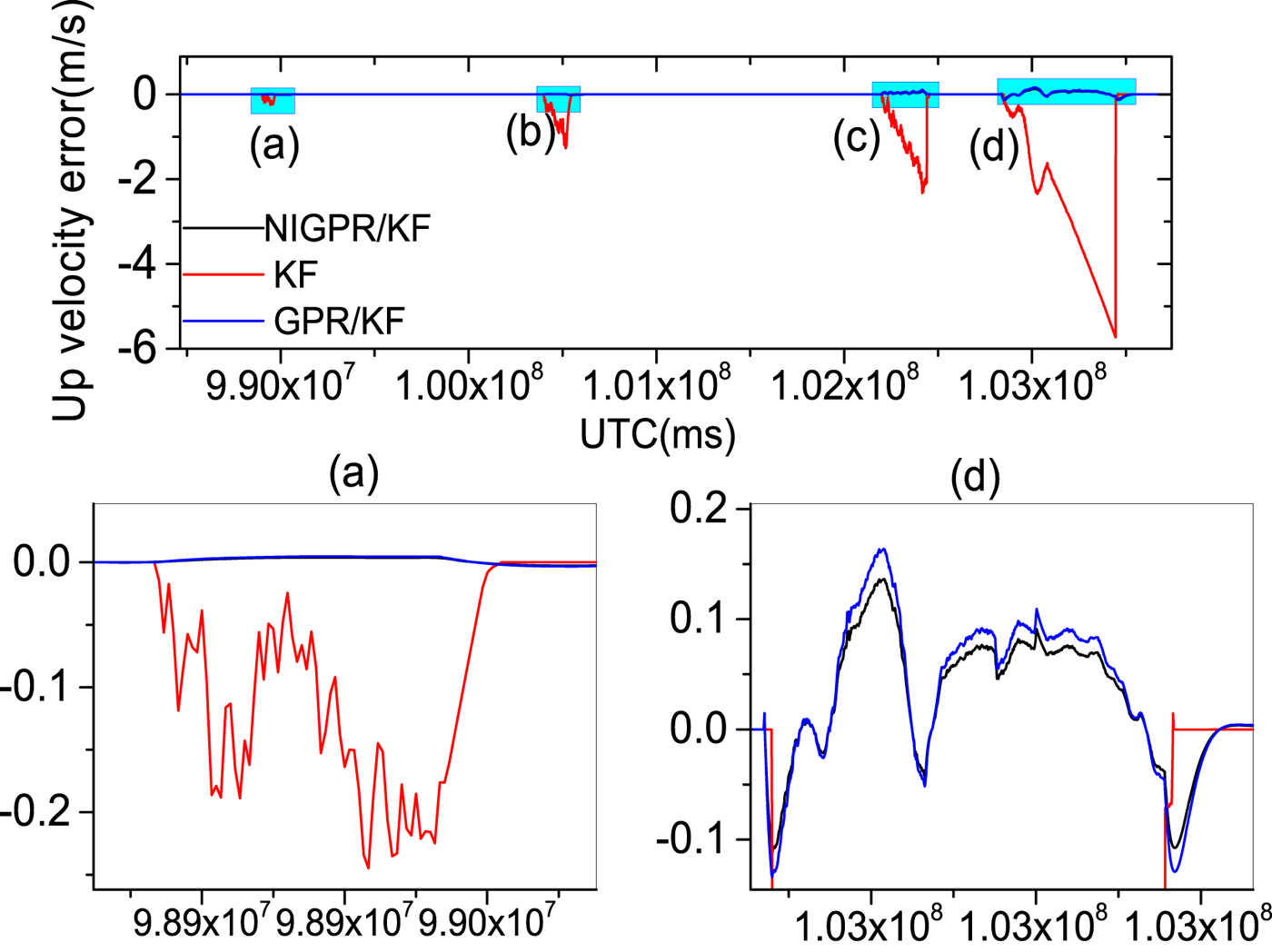
Figure 14. The top row is up velocity error curves; (a), (b), (c) and (d) represent the 60 s, 120 s, 240 s and 600 s GPS outages, respectively; in the second row, the panels (a) and (d) are the enlarged views of up velocity error corresponding to the GPS outages of 60 s and 600 s, respectively.
Obviously, the GPR/KF solution has a good performance in the cases of GPS outages mentioned. Table 3 shows that the position and velocity solutions obtained by the GPR/KF are distinctly superior to the KF solution. This is because the GPR/KF solution can describe the inherent nonlinear model of the INS error dynamics, which is related to the previous INS errors output and the sum of gyros and accelerometers measurements from time k−1 to k, respectively. Meanwhile, it adopts the a priori knowledge of the INS error dynamics. Once GPS outages occur, the predicted output of the GPR model is used to virtually update the KF. However, the GPR model assumes the input is noise-free, which is unlikely in the trained INS error dynamics model. The noise of the input is not considered, which may have an important effect on the performance of the predictor.
Table 3. RMS error of POS navigation using mentioned approaches during GPS outages.
Compared with the other two solutions mentioned in this paper, the proposed hybrid prediction solution shows the best performance during all the GPS outages. The main contribution of the proposed approach lies in utilising the NIGPR model based on the previous output of INS errors and the corresponding sum of the gyroscope and accelerometer measurements from time k−1 to k to accurately predict the pseudo  $Z_{prediction}^{k} $. It also uses the pseudo
  $Z_{prediction}^{k}$ to aid the POS KF, which adopts a priori knowledge of the INS error dynamics and takes the noisy input into consideration compared with the GPR/KF.
Table 3 shows the error statistics of the three solutions for four GPS outages with various lengths, and this shows the detailed quantitative analysis of POS errors. For the proposed hybrid predictor over 60 s, 120 s and 240 s outages, respectively, the position error is reduced by 92·6%, 98·5%, 96·8% and 97·1% compared with the KF solution. The Root Mean Squares (RMS) of latitude errors are 0·09 m, 0·26 m and 3·50 m, the RMS of longitude errors are 0·05 m, 0·25 m and 1·96 m; the RMS of altitude errors are 0·03 m, 0·20 m and 2·88 m and the RMS of velocity errors by 98·3%, 96·3%, 95·9% and 93.2%. Compared with the KF solution, the RMS of east velocity errors are 0·001 m/s, 0·01 m/s and 0·02 m/s, the RMS of north velocity errors are 0·001 m/s, 0·003 m/s and 0·05 m/s and the RMS of up velocity errors are 0·001 m/s, 0·001 m/s and 0·01 m/s. Likewise comparing with the GPR/KF solution, the improvement from the RMS of position error is more than 10%; regarding the RMS of velocity errors, their performance balances during short-term and middle-term GPS outages (60 s, 120 s and 240 s).
Since the NIGPR/KF model considers noise in the input, especially, during the 600 s outage, the RMS of position errors of the proposed hybrid prediction solution is still maintained below 23·80 m, which is considerably smaller than the KF solution (at 804 m) and slightly smaller than the GPR/KF solution (at 26 m). The RMS of velocity errors achieved are 0·34 m/s, 0·44 m/s and 0·05 m/s, which are an improvement of about 4·67 m/s, 4·79 m/s and 1·55 m/s compared with the KF solution. The NIGPR/KF model has improvements of about 0·04 m/s, 0·04 m/s and 0·01 m/s over the GPR/KF solution.
Although Table 3 illustrates the accuracy of the estimation for both the GPR/KF and NIGPR/KF solutions: they all degrade as the length of the GPS outage increases. The proposed hybrid (NIGPR/KF) technique offers a significant improvement over both the GPR/KF and the KF approaches. However, the accuracy of the NIGPR/KF technique is still limited by the amount of training data available.
5. CONCLUSION
In this work, we demonstrated how to model the error dynamics of an INS using Noisy Input Gaussian Process Regression (NIGPR) relying on historical flight data. The proposed approach has several significant properties, which make it ideally suited to the error dynamics of the INS and accurately predicts the measurement information for aiding the POS KF to acquire accurate position, velocity and attitude navigation information during various GPS outages. The performance of the proposed hybrid prediction approach was validated by a real flight test. Compared to the KF solution during GPS outages, the proposed approach has the best performance, which significantly reduces the errors of the stand-alone INS solution during artificial GPS outages of various lengths. Compared to the GPR/KF model, the proposed approach considers noise from inputs, which further improves the performance. Furthermore, the NIGPR model is based on both the sum of the gyro and accelerometer measurements and the previous INS error output, which is similar to the INS error dynamics model. Additionally, the combination with a priori knowledge of INS error dynamics can contribute to reducing the need for extensive training data.
However, if the proposed approach constrains the specific noise levels on each training data set to be the same, this would be computationally expensive. In fact, by fixing the input and output noise variances to be identical, the proposed approach is as computationally efficient as the standard GPR, which scales with the input vector dimension D 2. Our results showed that the proposed approach gives a substantial improvement over the standard GPR for modelling the INS error dynamics.
In future work, we will investigate how to detect GPS abnormality based on the short-term and high-precision FOG IMU, and then correct the measurement information and improve the traditional POS KF precision using a predictor relying on NIGPR, which may be a promising direction.
ACKNOWLEDGMENTS
This work is supported by the National High Technology Research and Development Program of China under Grant 2015AA124001 and 2015AA124002, National Nature Fund innovation group under Grant 61421063 and National Nature Fund under Grant 61473020, 61573040.