Benefit–cost analysis (BCA) evaluates a policy intervention by comparing the monetary value of the benefits to individuals who gain with the monetary value of the harms to individuals who lose. But there are two measures each of the monetary value of a benefit and of a harm to an individual: willingness to pay (WTP) for a benefit or to avoid a harm and willingness to accept compensation (WTA) to forgo a benefit or accept a harm. Under standard economic theory, in many circumstances the WTP and WTA measures of a benefit, and of a harm, should be nearly equal in magnitude and so the choice of which to employ should have little effect on the result of a BCA. In other circumstances, the two measures may be quite different and the choice between them may matter. Moreover, several decades of research in stated-preference and experimental economics has shown that empirical estimates of WTP and WTA often differ substantially, even in contexts where standard theory suggests they should be nearly equal. The disparity between WTP and WTA raises the question of which measures should be used, and when, in BCA.Footnote ¹

1. WTP and WTA

To fix ideas, consider a project that will affect the quantity of some public or other good $G$ available to individuals. Individuals cannot affect the quantity of $G$ they consume or have available, but it can be altered by public policy.

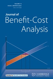
Figure 1 illustrates an individual’s indifference curves between $G$ and wealth or income that can be allocated for spending on all other goods. Consider first an individual at point $O$ with wealth $w$ and quantity $q$ for whom the policy will increase the quantity of $G$ to $q^{+}$ . Her WTP (compensating variation) for the increase is the amount $A$ , because the point $Y$ lies on the same indifference curve as her initial position $O$ . Her WTA to forgo the increase in the good (equivalent variation) is $B$ , because increasing her wealth from $w$ to $w+B$ holding quantity fixed at $q$ puts her at $Z$ , which is on the same indifference curve as increasing $q$ to $q^{+}$ while holding wealth fixed at $w$ (point $X$ ).

Figure 1 Four measures of value.

Next consider an individual who will be harmed by the policy. Assume the policy will reduce his quantity of $G$ from an initial level $q$ to a smaller level $q^{-}$ (although Figure 1 is drawn assuming the two individuals have identical wealth and initial levels of $G$ , this is not necessary and not true in general). The policy loser’s WTA (compensating variation) for the reduction in $G$ is $D$ and his WTP to prevent the reduction (equivalent variation) is $C$ .Footnote ²

If the indifference curves are vertically parallel, then the WTA and WTP measures for each individual are identical (i.e., $A=B$ and $C=D$ ).Footnote ³ Vertically parallel indifference curves imply that the slopes of the indifference curves may depend on $q$ but do not depend on $w$ ; in other words, the marginal rate of substitution between wealth and $G$ may depend on the quantity of $G$ but not on wealth. This implies that the income elasticities of WTP and of WTA are zero.Footnote ⁴

If WTA to forgo an improvement is greater than WTP for the improvement from $q$ to $q^{+}$ , then the higher indifference curve is steeper on average between $Z$ and $X$ than the original indifference curve between $O$ and $Y$ . Equivalently, the income elasticities of WTP and of WTA are larger (on average) when income is larger (for values of $G$ between $q$ and $q^{+}$ ).

For many goods, it is reasonable to assume that the income elasticity of WTP is positive, so WTA is larger than WTP. But for small changes in the quantity of $G$ , it seems intuitive that the indifference curves must be nearly parallel (they cannot cross), which implies WTP must be nearly equal to WTA. This intuition is not strictly accurate, however. Hanemann (Reference Hanemann1991) shows that the difference between WTP and WTA can be arbitrarily large, even for a small change in the quantity of $G$ , if $G$ has no close market substitutes. The intuition is that if there is a close market substitute for $G$ (either a single good or a basket of goods), then an individual for whom the quantity $q$ is not optimal can adjust by purchasing more or less of the substitute market good, so her consumption of $G$ plus its market substitute is optimal. If the market substitute is available at a fixed price, this priceFootnote ⁵ equals her marginal WTP and WTA for a change in $G$ and her indifference curves between wealth and $G$ are parallel straight lines. In contrast, if there is no close market substitute for $G$ , the consumer cannot adjust for a non-optimal quantity and her indifference curves may be arbitrarily far from vertically parallel.Footnote ⁶

The empirical finding that estimated WTA is often much larger than estimated WTP implies either that the indifference curves are not approximately vertically parallel over the relevant domain, or that the empirical method is not accurately estimating these monetary values. A number of hypotheses have been suggested to explain this disparity (Mitchell & Carson, Reference Mitchell and Carson1989). In addition to Hanemann’s (Reference Hanemann1991) result concerning the absence of market substitutes for the good, other explanations include income effects and transaction costs (Randall & Stoll, Reference Randall and Stoll1980), uncertainty about and caution in revealing one’s true WTP or WTA, commitment costs (loss of opportunity to learn about the value of a good before acting; see Zhao & Kling, Reference Zhao and Kling2004), and limited incentives to learn about preferences for a hypothetical transaction (Guzman & Kolstad, Reference Guzman and Kolstad2007).

Other explanations depart from the standard economic model such as reference dependence, loss aversion, or other endowment effects (Thaler, Reference Thaler1980; Kahneman, Knetsch & Thaler, Reference Kahneman, Knetsch and Thaler1990). For example, if people characterize a change in $G$ as in the domain of gains or losses relative to some reference level and are more averse to losses than to gains, then the value of a specific change in $G$ may depend on the reference level (Knetsch, Reference Knetsch2010; Knetsch, Riyanto & Zong, Reference Knetsch, Riyanto and Zong2012). Reference dependence implies that individuals do not have indifference curves that are defined over consequences alone, like those in Figure 1, but rather sets of indifference curves over consequences that are conditional on alternative reference levels.

Alternatively, some authors claim that the disparity is due to experimental-design features and elicitation techniques such as the use of elicitation methods that are not incentive compatible (e.g. Plott & Zeiler, Reference Plott and Zeiler2005, Reference Plott and Zeiler2007). Isoni, Loomes and Sugden (Reference Isoni, Loomes and Sugden2011) find that strong experimental procedures eliminate the disparity for some goods, but not for others. There is no consensus on why a large gap between the two values is often observed.

An important question for BCA is whether the observed differences between WTA and WTP represent individuals’ informed, normative preferences or reflect cognitive errors or limitations of the methods used to estimate these values (Hammitt, Reference Hammitt2013). Three meta-analyses of the empirical literature reveal that the difference between WTP and WTA varies systematically with characteristics of the good that is valued and the valuation method. In their pioneering meta-analysis of 45 studies, Horowitz and McConnell (Reference Horowitz and McConnell2002) evaluated the effects of the type of good that was valued and the strength of the experimental design. They found the type of good is systematically related to the WTP–WTA disparity, with smaller disparities for ordinary private goods than for public goods or other goods that are not usually available in markets. They found little evidence that weak experimental design contributes to a larger disparity; e.g., they found no systematic difference in the disparity between studies using hypothetical and real transactions and, surprisingly, that the disparity is significantly smaller for studies using non-incentive-compatible elicitation mechanisms. They also found a smaller disparity in studies using student subjects. The second meta-analysis, of 39 studies by Sayman and Onculer (Reference Sayman and Onculer2005), found that the use of an incentive-compatible elicitation mechanism decreases the disparity.

The third meta-analysis, of 76 studies by Tunçel and Hammitt (Reference Tunçel and Hammitt2014), reinforces and refines these conclusions. Tunçel and Hammitt found a systematic relationship between the magnitude of the disparity and the type of good valued, with a geometric-mean ratio of WTA to WTP of about 6 and 5 for environmental goods and for health and safety, respectively, and of about 1.5 for ordinary private goods and for travel or leisure time. They found the disparity is smaller for experiments using incentive-compatible elicitation mechanisms and also smaller when participants have prior experience buying or selling the good or when they have gained experience through participating in multiple elicitation rounds as part of the study. They also found the disparity is on average smaller in more recent studies; in part this reflects improvements in experimental design but a statistically significant effect remains even after controlling for design features. Tunçel and Hammitt tested Hanemann’s (Reference Hanemann1991) suggestion that the disparity could be larger for goods lacking close substitutes by including a variable reflecting their judgment about whether market substitutes exist. They found some evidence supporting this hypothesis, but the existence of substitutes is confounded with the type of good, as almost all ordinary private goods have close substitutes. They found no statistically significant association of the WTA/WTP ratio with the absence of market substitutes when restricting the analysis to goods that are not ordinary private goods.

2. Implications for BCA

Large positive differences between estimated WTA and WTP measures of the value of a benefit, or the value of a harm, tend to accentuate the ambiguity that can arise under the conventional justification for BCA, the Kaldor–Hicks compensation test. The compensation test is composed of two criteria: the Kaldor criterion uses compensating variations; it classifies the policy intervention as socially beneficial if the total WTP of those who gain exceeds the total WTA of those who are harmed. A large difference between WTA and WTP will make this criterion more difficult to satisfy, hence favoring the status quo over the policy intervention. In contrast, the Hicks criterion uses equivalent variations; it classifies the policy intervention as socially beneficial if the total WTP to prevent the intervention of those who are harmed is less than the total WTA to forgo the intervention of those who gain. A large difference between WTA and WTP makes this criterion easier to satisfy, hence favoring the intervention over the status quo. Combining these two effects, a large difference between WTA and WTP makes it more likely that the Kaldor–Hicks compensation test is ambiguous: gainers cannot compensate losers for the intervention and losers cannot compensate gainers to forgo the intervention.

One resolution to a contradiction between the Kaldor and Hicks criteria in a specific case is to recognize that the appropriate test may depend on property rights (Mitchell & Carson, Reference Mitchell and Carson1989; Freeman, Reference Freeman1993). If those who would be harmed by a policy intervention have a legal right to avoid that harm, then the Kaldor criterion is appropriate; if those who would benefit have a right to that gain, then the Hicks criterion is appropriate. As an example, assume that hunters (or hikers) use some parcel of undeveloped land and a dam is proposed that would flood the land. If the hunters have a legal right to their use of the land, because of ownership, custom, or other reasons, the dam should not be built unless the WTP of those who gain exceeds the hunters’ WTA for their loss of access. Alternatively, if the hunters are trespassers with no right to their use, the dam should be built unless their WTP to prevent construction exceeds the WTA of those who benefit from the dam.

Knetsch (Reference Knetsch2010) suggests a modification of this property-rights approach, in which the reference point (in the example, whether the hunters are entitled to their use) depends not necessarily on legal rights but on what people identify as the normal or expected state or on their legitimate expectations. For example, he suggests that in evaluating whether to remediate a toxic-waste spill, the situation without the spill is the natural reference and so the Hicks criterion is relevant: the test for whether the spill should be remediated is whether WTP to avoid cleanup by the responsible party exceeds WTA to forgo cleanup by the beneficiaries, not whether the beneficiaries’ WTP for remediation exceeds the costs to the responsible party.

For many public policies, resolving the ambiguity by designating either the Kaldor or the Hicks criterion as definitive based on considerations of rights or legitimate expectations seems inadequate. In some important cases, the benefits and costs of a policy are imposed on the same people. For example, the costs of policies to improve product or transportation safety are likely to be passed on to the beneficiaries through higher prices of the specific goods or services. Similarly, the benefits of reduced air pollution will tend to be broadly distributed over a regional population and the costs in the form of higher prices for electricity or fuels may also be broadly distributed over the same population. Even in the example of remediating a toxic-waste spill, while the responsible party may bear the cost of cleanup, the long-run effect may be that firms exercise more care to prevent toxic-waste spills and pass the costs on to their consumers; so in the long run the gainers and losers may substantially overlap.Footnote ⁷ Although the population distributions of benefits and costs need not be the same, in each of these cases it is likely that most individuals receive some benefits and bear some costs, so it is necessary to evaluate the net effect on each person to determine who benefits and who is harmed. Estimating benefits and costs separately is not sufficient.

In cases where both benefits and costs are incurred by the same people, each individual must prefer either the policy or its absence (or be indifferent between them). If an individual’s judgment about whether he favors the policy is dependent on whether he asks himself whether his WTP for the benefit is less than the cost he will bear or his WTA compensation to forgo the project exceeds the cost he will save, then he is incoherent and may be easily manipulated by clever policy advocates.

An individual’s choice can be correctly framed using either WTP or WTA, but the relevant comparison is not the comparison between $A$ and $B$ that is illustrated in Figure 1. If the individual has initial quantity of the good $q$ and wealth $w$ , he can compare his WTP for the increase in $G$ from $q$ to $q^{+}$ (the quantity $A$ in Figure 1) with the cost he will bear. Alternatively, he can compare his WTA to forgo the increase in $G$ with the cost he will save. This is not the amount $B$ illustrated in Figure 1, but is his WTA to forgo the increase from $q$ to $q^{+}$ when his wealth is $w$ less than the cost he will bear. Suppose the cost he will bear is $A$ , so his WTP for the increase in $G$ equals the cost and he is indifferent to the policy. Then his WTA to forgo the increase from $q$ to $q^{+}$ when his wealth is $w-A$ is exactly $A$ , and this alternative framing also reveals him to be indifferent to the policy.

With reference-dependent preferences, if WTP for the increase uses $q$ as the reference and WTA to forgo the increase uses $q^{+}$ as the reference then the results of these alternative framings may be inconsistent – but that suggests the individual must somehow reconcile the different perspectives. Alternatively, if the reference-dependent preferences are normative, this introduces another source of uncertainty into BCA: the analyst will generally not know the individual’s reference level and hence how the change in $G$ should be valued. The reference level can be interpreted as an ancillary condition that may affect an individual’s choices but is not known by the analyst, leading to ambiguity about the preferences that are revealed by his choices (Bernheim & Rangel, Reference Bernheim and Rangel2009).

In other cases, the individuals who benefit or are harmed by a policy may be distinct and the Kaldor and Hicks criteria may conflict. This conflict can arise even if the differences between WTA and WTP are small, but will arise for a larger set of policies when the differences are large. These are cases in which the policy has a distributional effect that is comparable to the efficiency effect, in the sense that whether the estimated net benefits are positive or negative is sensitive to whether one treats the gainers’ or losers’ consequences as primary (e.g., as being favored by legal right or legitimate expectation). In these cases, debating the relative merits of the Kaldor and Hicks criteria seems to obscure rather than elucidate the fundamental question, which is whether the benefits to the gainers justify imposing the harms on the losers. It seems likely that a better resolution may be achieved by addressing this question directly. The answer to whether the distributional consequence is justified may, of course, depend on legal rights and legitimate expectations.