


Introduction
Plumes of large rivers affect coastal and oceanic areas both at regional and continental scales, as well as at the global scale, and they play an important role in the hydrological cycle and thermodynamic stability of the ocean (Dagg et al., Reference Dagg, Benner, Lohrenz and Lawrence2004; Chérubin & Richardson, Reference Chérubin and Richardson2007). In northern Brazil, the tropical Atlantic receives the drainage from the Amazon River, which accounts for ~20% of the total global freshwater discharge, within a complex, megascale delta (Nittrouer et al., Reference Nittrouer, Kuehl, Demaster and Kowsmann1986; Mikhailov, Reference Mikhailov2010). The interaction between river discharges from the Amazon system and the action of strong trade winds and surface ocean currents controls the pelagic processes in the northern coast of Brazil, affecting physico-chemical dynamics, as well as planktonic distribution and biomass on the Amazon continental shelf (Dagg et al., Reference Dagg, Benner, Lohrenz and Lawrence2004; Santos et al., Reference Santos, Muniz, Barros-Neto and Araujo2008; Molleri et al., Reference Molleri, Novo and Kampel2010; Goes et al., Reference Goes, Gomes, Chekalyuk, Carpenter, Montoya, Coles, Yager, Berelson, Capone, Foster, Steinberg, Subramaniam and Hafez2014; Conroy et al., Reference Conroy, Steinberg, Stukel, Goes and Coles2016; Santana et al., Reference Santana, Lira, Varona, Neumann-Leitão, Araujo and Schwamborn2020).
In large-scale tropical continental shelf environments, the diversity of organisms derives from an extensive coast with diverse marine and estuarine habitats (mangrove forests, marshes, coral reefs). In the north of Brazil, the junction of the outflowing rivers Amazon and Pará converts the ACS into an important nursery and growth area for marine and estuarine shrimps (Dall et al., Reference Dall, Hill, Rothlisberg, Sharples, Blaxter and Southward1990; Dagg et al., Reference Dagg, Benner, Lohrenz and Lawrence2004; Nascimento et al., Reference Nascimento, Souza-Filho, Proisy, Lucas and Rosenqvist2013; Cordeiro et al., Reference Cordeiro, Neves, Rosa-Filho and Pérez2015; Moura et al., Reference Moura, Amado-Filho, Moraes, Brasileiro, Salomon, Mahiques, Bastos, Almeida, Silva, Araujo, Brito, Rangel, Oliveira, Bahia, Paranhos, Dias, Siegle, Figueiredo, Pereira, Leal, Hajdu, Asp, Gregoracci, Neumann-Leitão, Yager, Francini-Filho, Fróes, Campeão, Silva, Moreira, Oliveira, Soares, Araujo, Oliveira, Teixeira, Valle, Thompson, Rezende and Thompson2016).
Larval stages are the primary means for geographic dispersal of marine shrimps. During this phase, distribution is affected by temperature, salinity, rainfall, winds and currents, among others (Anger, Reference Anger2001, Reference Anger2006). These characteristics, together with food availability, competition and predation, are the major factors responsible for seasonal variation and recruitment levels in the adult population (Anger, Reference Anger2001). Hence, a successful life history strategy depends mostly on the survival of planktonic larvae (Anger, Reference Anger2006).
Shrimps represent an important group for marine ecosystems both in their larval phase, as a component of the plankton and trophic pyramid, and in their benthic/nektonic phase, where they act as omnivores or detritivores that play an important role in nutrient cycling and energy flow, serving as the main energy pathway from primary producers to higher trophic level organisms, such as fish. They obtain nutrients from dead organisms or part of them, making nutrients available to predators, constituting an important link in the aquatic trophic web. However, information on the distribution of shrimp larval stages or even of juveniles and adults as a component of zooplankton is scarce in the north Brazilian shelf.
There are 30 shrimp species of the suborder Dendrobranchiata reported on the Amazon continental shelf (ACS) and nearby estuarine areas: 5 Sergestoidea species (2 Luciferidae and 3 Sergestidae) and 25 Penaeoidea species (3 Aristeidae, 12 Penaeidae, 6 Sicyoniidae and 4 Solenoceridae) (D'Incao, Reference D'Incao1997, Reference D'Incao and Young1998; Barros & Pimentel, Reference Barros and Pimentel2001; Silva et al., Reference Silva, Muniz, Ramos-Porto, Viana and Cintra2002a, Reference Silva, Ramos-Porto, Cintra, Muniz and Silva2002b, Reference Silva, Cintra, Ramos-Porto, Viana, Abrunhosa and Cruz2020; Costa & Costa, Reference Costa and Costa2008; Melo et al., Reference Melo, Neumann-Leitão, Gusmão, Martins-Neto and Palheta2014; Pimentel & Magalhães, Reference Pimentel and Magalhães2014).
Luciferidae comprises holoplanktonic species that might account for up to 15% of planktonic biomass on tropical continental shelves due to their size (Longhurst, Reference Longhurst1985), and all life stages are found on the ACS (Melo et al., Reference Melo, Neumann-Leitão, Gusmão, Martins-Neto and Palheta2014; Conroy et al., Reference Conroy, Steinberg, Stukel, Goes and Coles2016; Neumann-Leitão et al., Reference Neumann-Leitão, Melo, Schwamborn, Diaz, Figueiredo, Silva, Campelo, Melo Júnior, Melo, Costa, Araújo, Veleda, Moura and Thompson2018). Sergestidae includes pelagic or benthopelagic shrimps that inhabit estuaries and tropical, subtropical and temperate coastal waters, which have high abundance formed by aggregations in certain periods of the year (Omori, Reference Omori1975; Xiao & Greenwood, Reference Xiao and Greenwood1993).
Penaeoidea are meroplanktonic with only larval stages found in zooplankton. In general, four types of migratory movements might be observed (based on Penaeidae): (1) migration of larvae and post-larvae to nursery areas (estuaries, mangroves, lagoons); (2) migration of juveniles outside the nursery area (towards the ocean, shelf); (3) migration of adults, generally towards deeper waters in the sea/ocean; and (4) migration only for spawning in some species (Dall et al., Reference Dall, Hill, Rothlisberg, Sharples, Blaxter and Southward1990). Although penaeid larvae usually migrate from the ocean towards the estuary, where juveniles will develop until they return to the sea as adults (Dall et al., Reference Dall, Hill, Rothlisberg, Sharples, Blaxter and Southward1990), the life cycles of Aristeidae, Solenoceridae and Sicyoniidae shrimps are exclusively marine (Gomez-Ponce & Gracia, Reference Gomez-Ponce and Gracia2003; Castilho et al., Reference Castilho, Furlan, Costa and Fransozo2008; Kapiris & Thessalou-Legaki, Reference Kapiris and Thessalou-Legaki2009; Pezzuto & Coachman-Dias, Reference Pezzuto and Coachman-Dias2009; Simões et al., Reference Simões, Heckler and Costa2017; Garcia et al., Reference Garcia, Lopes, Silvestre, Grabowski, Barioto, Costa and Castilho2018).
Ecological studies about planktonic shrimps on the ACS are still scarce and have limited availability, as they consist of unpublished monographs, theses and dissertations, all of which are based on single cruises, with no seasonality reports. One of the only studies conducted about planktonic shrimp published as a manuscript was by Melo et al. (Reference Melo, Neumann-Leitão, Gusmão, Martins-Neto and Palheta2014), who analysed the distribution of luciferid juvenile and adult shrimps along neritic and oceanic environments on the Amazon shelf, and recently Santana et al. (Reference Santana, Lira, Varona, Neumann-Leitão, Araujo and Schwamborn2020) analysed the abundance and composition of planktonic decapod communities along the Amazon River plume and its retroflection. Therefore, nothing is known about the larval stages of dendrobranchiate on the ACS.
Based on the complexity of the ACS system and the dynamic character of the zooplankton, this study attempted to answer the following questions: which dendrobranchiate shrimps are found as the dominant planktonic components on the ACS? How are these four groups (penaeoid larvae and sergestoid larvae, juveniles and adults) spatially distributed in an area under the influence of the plumes of the Amazon and Pará rivers? Are there differences in the distribution of occurrence of shrimp larval stages? Which environmental factors primarily affect the spatial-temporal distribution of these groups?
Considering that freshwater supply in coastal areas depends on a highly variable estuarine plume, shrimp survival and development would be affected. This study hypothesized that there is a difference in the distribution of shrimp groups on the ACS related to seasonality and the coast–ocean gradient, since there are different migratory patterns depending on groups, and different tolerances to salinity variations. Thus, different distribution patterns of planktonic shrimp were expected.
Method
Study area
The Atlantic Ocean receives the discharges of the Amazon and Pará Rivers into a complex megascale delta (Nittrouer et al., Reference Nittrouer, Kuehl, Demaster and Kowsmann1986). The Amazon River Basin, considered the largest in the world, extends from the Andes until the Atlantic Ocean and covers an area of ~7 × 10⁶ km2 (Dagg et al., Reference Dagg, Benner, Lohrenz and Lawrence2004; Molleri et al., Reference Molleri, Novo and Kampel2010), discharging 940 × 106 t/year of sediments and 180,000 m3 s−1 of fresh water into the Atlantic Ocean (Muller-Karger et al., Reference Muller-Karger, McClain and Richardson1988; Mikhailov, Reference Mikhailov2010). In northern Brazil, the shelf break zone of the ACS is between 90 and 100 m depth (Nittrouer & DeMaster, Reference Nittrouer and DeMaster1996), and the inner shelf is limited by the 20-m isobath, with a deeply jagged coastline encompassing the largest continuous strip of mangrove forests in the world (Nascimento et al., Reference Nascimento, Souza-Filho, Proisy, Lucas and Rosenqvist2013).
The Amazon River outflow varies seasonally, ranging from ~220,000 m3 s−1 in May (maximum flooding of the river) to 100, 000 m3 s−1 in November (low flow period) (Geyer et al., Reference Geyer, Beardsley, Lentz, Candela, Limeburner, Johns, Castro and Soares1996; Silva et al., Reference Silva, Santos, Araujo and Bourlès2009; Molleri et al., Reference Molleri, Novo and Kampel2010), and it forms a low-salinity surface plume that extends along the shelf, transported primarily north-westwards by the North Brazil Current (Muller-Karger et al., Reference Muller-Karger, McClain and Richardson1988; Geyer et al., Reference Geyer, Beardsley, Lentz, Candela, Limeburner, Johns, Castro and Soares1996). There is only one rainy season in this region, from December to May (period of maximum flood of the Amazon River), and a less rainy season, from June to November (dry season or low flow period of the Amazon River) (Rao & Hada, Reference Rao and Hada1990).
The North Brazil Current (NBC) transports warm surface waters to the north and flows along the ACS shelf break and slope (Richardson et al., Reference Richardson, Hufford, Limeburner and Brown1994). The NBC has a large annual cycle, concurrent with changes in wind speed, ranging from a maximum transport of 36 × 106 m3 s−1 in July–August (maximum winds in the dry season) to a minimum transport of 13 × 106 m3 s−1 in April–May (weak winds in the rainy season), with an annual mean transport of ~26 × 106 m3 s−1 (Johns et al., Reference Johns, Beardsley, Candela, Limeburner and Castro1998). It changes direction along the Brazilian northern coastline according to wind patterns and to position of the Amazon plume (Ffield, Reference Ffield2005). The predominance of the Amazon River plume near its mouth occurs in the first half of the year, coinciding with the higher river outflow and with weaker north-eastern trade winds. In the oceanic area, plume displacement is related to currents, moving north-eastwards via the NBC towards the Caribbean Sea. Near the State of Amapá, this current seasonally undergoes a large-scale eastward retroflection towards Africa in the second semester, feeding the Equatorial North Counter-Current (ENCC) (Muller-Karger et al., Reference Muller-Karger, McClain and Richardson1988; Ffield, Reference Ffield2005; Silva et al., Reference Silva, Santos, Araujo and Bourlès2009).
Sampling and sample processing
Samplings were performed seasonally, seven times in three-month intervals, from July 2013 to January 2015, along a transect with six sampling sites on the Amazon continental shelf, starting from the coastline (at Marajó Island) and going as far as ~250 km off the coast on the slope, encompassing a full large-scale transect along an ocean–estuarine continuum (Figure 1). The distance from the sampling sites to the coast was ~23 km (site 1), 53 km (site 2), 83 km (site 3), 158 km (site 4), 198 km (site 5) and 233 km (site 6). Samplings were conducted using a fishing boat equipped with radio, depth probe, GPS and a winch for plankton hauls. Before capturing the zooplankton, a CTD-probe (Hydrolab DS 5) was used to record the abiotic factors and make profiles of each parameter of the water column: temperature (°C), salinity and chlorophyll-a (μg l−1).
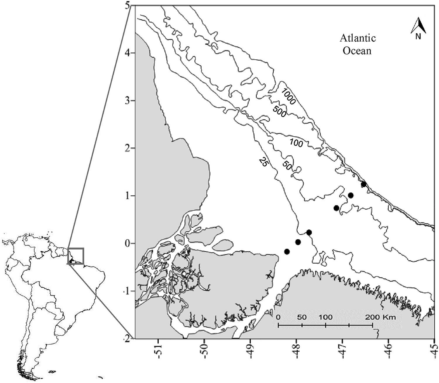
Fig. 1. Amazon continental shelf: the black dots represent the sampling sites in the period ranging from July 2013 to January 2015.
Samples were obtained with a conical-cylindrical plankton net (200 μm mesh and 30 cm diameter), with a flow meter coupled to the net opening. The samplings were from surface to bottom, one sample per station, with oblique hauls down to 75% of local depth (~10, 19, 34, 39, 53 and 80 m depth), and at each depth they were hauled for 5 min. The total duration of the hauls varied from 10–20 min, at a speed of approximately 2 knots. Samples were fixed in 4% formaldehyde, previously buffered with sodium tetraborate. In the laboratory, samples were fractioned with a Folsom sub-sampler, and a fraction of half of the initial sample was used to screen the shrimps. A total of 42 samples were analysed: 7 expeditions throughout 2 years (July/13, October/13, January/14, May/14, July/14, October/14, January/15) × 6 sites on the ACS.
Mysis larval stages, decapodids (post-larva), juveniles and adults (the latter two were only Sergestoidea) were identified using specialized references (Brooks, Reference Brooks1882; Cook, Reference Cook1964; Boschi, Reference Boschi and Boltovskoy1981; Calazans, Reference Calazans1993; Oshiro & Omori, Reference Oshiro and Omori1996; Dos Santos & Lindley, Reference Dos Santos, Lindley and Lindley2001). Nauplii and protozoea stages were not counted as the abundance of these small larvae was underestimated by the 200-micron net mesh. The organisms were counted and identified under an optical stereomicroscope (ZEISS StereoDiscovery v.12) and dissected using an optical microscope equipped with a micrometric disc.
Data analysis
Amazon River outflow data were obtained from the Brazilian Hidroweb service (http://www.snirh.gov.br/hidroweb/) based on data from the Óbidos-Pará station provided by the Brazilian National Water Agency (ANA). Due to the huge scale of the Amazon basin, river discharge seasonality at the river mouth is mostly affected by rain in upstream areas, and not by the seasonal timing of rainfall on the coast. The variables ‘outflow’ (m3 s−1), ‘temperature’ (°C), ‘salinity’ and ‘chlorophyll-a’ (μg l−1) were tested using Shapiro–Wilk (k samples) and Levene's tests, and did not have normality and homoscedasticity, respectively. Thus, variation in outflow between months could be compared using Kruskal–Wallis ANOVA, as well as other abiotic factors among distance to the coast and months, all of which were followed by Student–Newman–Keuls (SNK) post hoc test.
Spatial variation in temperature (°C), salinity and chlorophyll-a (μg l−1) was represented by contour maps, elaborated using Surfer® 9.0 (Golden Software Inc., 2005). The krigage interpolation method was used due to its higher precision, because it is more faithful to the data, and due to its better curve smoothness compared with other methods (Landim, Reference Landim2003). Isolines related to the environmental factors mentioned above were highlighted, and salinity was categorized according to Seidel et al. (Reference Seidel, Yager, Ward, Carpenter, Gomes, Krusche, Richey, Dittmar and Medeiros2015) in salinity ranges (S) that characterize the Amazon River plume: inner or estuarine plume (0 < S ≤ 20), intermediate plume (20 < S ≤ 31), outer plume (31 < S ≤ 36), and ocean waters (S > 36).
The number of shrimps found in the aliquoted volumes was multiplied by the corresponding subsampling factor and the shrimp density was estimated in number of individuals per m3 (ind m−3). Frequency of occurrence was calculated considering the number of samples in which each taxon occurred compared with the total number of samples, and taxa were grouped in four categories: very frequent (>70%), frequent (≤70 and ≥40%), infrequent (<40 and ≥10%) and rare species (<10%) (Melo, Reference Melo2004 adapted from Mateucci & Colma, Reference Mateucci and Colma1982). The frequency of occurrence of shrimps was also calculated according to distance from the coast and was compared using the chi-square test, testing the hypothesis of increasing (A > 0) or decreasing tendency (A < 0) in the proportion of these frequencies, using BioEstat® 5.0 (Ayres et al., Reference Ayres, Ayres, Ayres and Santos2007).
Even after transformation, shrimp densities did not meet the criteria to perform parametric tests. Therefore, Kruskal–Wallis ANOVA was used to compare the variation in shrimp density among months and distances from the coast. Shrimp density was compared between years and periods with higher vs lower Amazon River outflow using pairwise Mann–Whitney tests. These univariate analyses were performed using Statistica® 12.7 (Statsoft Inc., 2015), with a significance level of 5%.
A Redundancy Analysis (RDA) was performed according to Borcard et al. (Reference Borcard, Gillet, Legendre, Gentleman, Hornik and Parmigiani2011), using the ‘vegan’ package in R (Oksanen et al., Reference Oksanen, Blanchet, Friendly, Kindt, Legendre, McGlinn, Minchin, O'Hara, Simpson, Solymos, Stevens, Szoecs and Wagner2017), to analyse shrimp assemblage distribution concerning explanatory variables (environmental factors, months and distance from the coast). For this analysis, the environmental data matrix (outflow, salinity, temperature and chlorophyll-a) was transformed using the ‘Standardization’ method, and shrimp density matrix (per development stages and families) was transformed using the Hellinger method. The latter is recommended for species abundance data clusters or ordinations, since it is not influenced by matrix zeros and it lowers the importance of more abundant groups (Legendre & Birks, Reference Legendre, Birks, Birks, Lotter, Juggins and Smol2012). Subsequently, a permutation ANOVA (PERMANOVA) was performed to test the significance of the RDA model, with 999 permutations, adopting the significance level of 5%.
Results
Abiotic factors
The highest Amazon River outflow (291,900 m3 s−1) was in May (2014) and the lowest (~110,000 m3 s−1) was in October (2013 and 2014). River outflow significantly differed among months (H (df = 6; N = 217) = 195.75; P < 0.01); May and July 2014 had the maximum river discharges, and the outflow in May 2014 was significantly higher than the rest of the study period. October (2013 and 2014) showed the lowest discharges, the beginning of the river level descent process occurred in July 2013, and discharge started to increase in January (2013 and 2014). Only January (both years) showed values within the historical mean from 1985 to 2015, while the other months showed somewhat higher discharges (Figure 2).
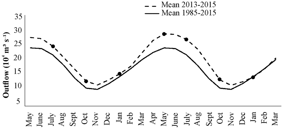
Fig. 2. Mean daily Amazon River outflow in the study period (July 2013 to January 2015) and in the last 30 years (1985–2015). The black dots indicate the sampling months on the Amazon continental shelf.
Sea temperatures ranged from 22–30 °C and remained above 27 °C on the majority of the shelf. Temperature also differed according to coast–ocean distance (H (5; 1434) = 748.30; P < 0.01). The lowest temperatures were recorded starting 200 km away from the coast and only at the deepest sites (Figure 3). Temperature significantly varied among months (H (6; 1434) = 287.89; P < 0.01); July (2013 and 2014), with high discharge, had the highest mean temperatures and January and October/14 had the lowest, coinciding with low river discharge (Figure 4).
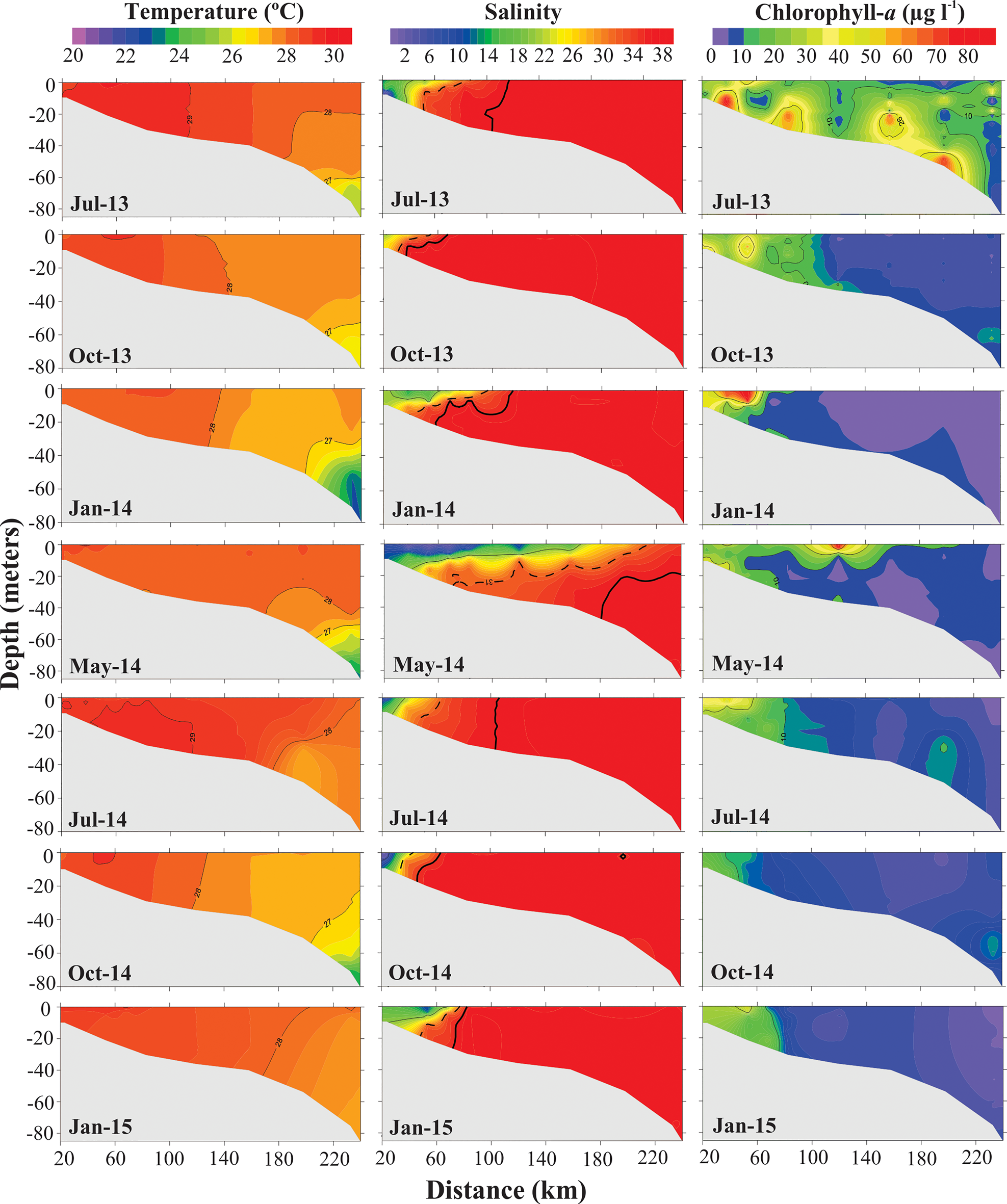
Fig. 3. Temperature (°C), salinity, and chlorophyll-a (μg l−1) in the water column of the Amazon continental shelf (2013–2015). For salinity: estuarine range (up to the full line), inner plume range (between the full line and the dashed line), outer plume range (between the dashed line and the thicker line), and oceanic range (from the thicker line outwards).
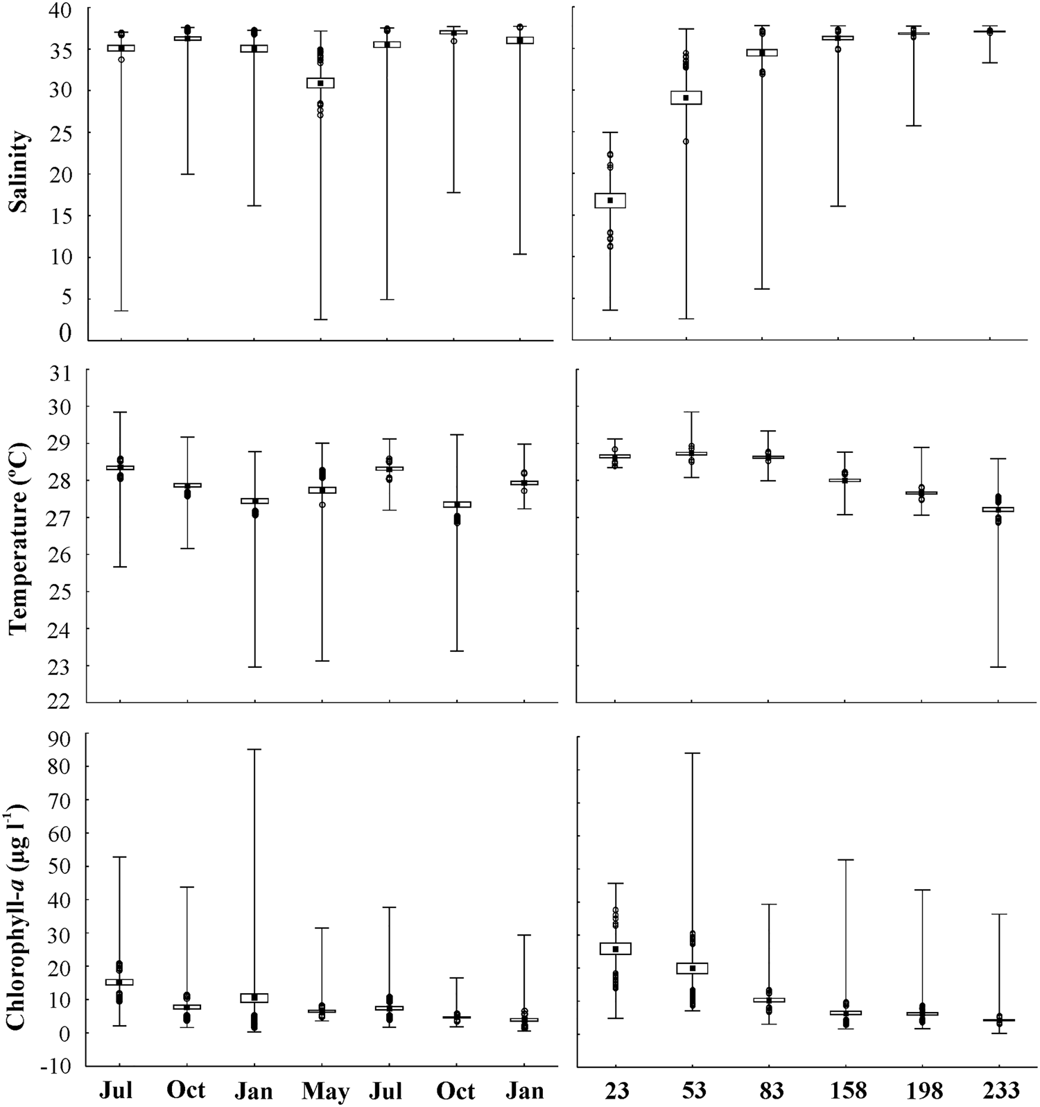
Fig. 4. Minimum and maximum values, outliers, mean and standard error of abiotic factors in relation to months and distance from the coast on the Amazon continental shelf (2013–2015).
Salinity varied from 2 to 38; the lowest values were recorded in May (mean value of 30.93 ± 8.89 SD), along with the period of highest Amazon River outflow, and the highest values were recorded in October (37.02 ± 2.79) (H (6; 1407) = 674.66; P < 0.01), the period with the lowest river outflow (Figure 4). Regarding coastal-offshore gradients, the lowest mean salinities were recorded near the shore, at a 23 km distance from the coast (H (5; 1407) = 314.08; P < 0.01) (Figure 4). The shelf was under the influence of low-salinity plume waters in all months, which was evident as far as 150 km distance. Farther than 150 km, salinity was >36 during most of the sampling period. Low-salinity plume waters showed a longer extension in May/2014, exceeding 200 km of distance on the ACS, and a shorter extension in October, where the plume reached as near as ~60 km (Figure 3).
Chlorophyll-a varied from 0.3 μg l−¹ (~41 m depth, 233 km from coast) to 85.1 μg l−¹ (~0.5 m depth, 53 km from coast), both in January 2014, in the onset of the rainy season. Mean chlorophyll-a values were significantly higher in July 2013 and January 2014 (15.2 and 10.5 μg l−¹, respectively) (H (6; 1383) = 288.60; P < 0.01), while they were higher in the more superficial layers in January 2014 (0.5–6.5 m depth at 53 km from the coast).
Overall, chlorophyll-a showed a similar spatial extent along the low-salinity plume, with significant variations along the coast–ocean distance (H (5; 1383) = 567.65; P < 0.01). The largest spatial extent of remarkably high chlorophyll-a values occurred in July 2013 and May 2014, along the entire water column, reaching farther than 200 km and with very high values (>20 μg l−¹). In the other months, it remained more concentrated near the coast (as near as ~100 km) and in more superficial layers (only down to 20 m depth). The lowest values (<5 μg l−¹) occurred far away from the coast and at deep layers (Figures 3 and 4).
Abundance and distribution of Dendrobranchiata shrimps
In the present study 14,057 specimens of dendrobranchiate planktonic shrimps were analysed, belonging to five families and nine taxa (Supplementary Table S1). Luciferidae shrimps (13,065 specimens) and the mysis stage (8078 larvae) were the most abundant among the dendrobranchiate shrimps. The total density of shrimps presented a mean of 2.18 ± 6.26 ind m−3. They were present throughout the study period with higher mean in May 2014 (9.09 ± 15.37 ind m−3) followed by October 2013 (2.11 ± 3.15 ind m−3). The lowest mean density was in July 2013 (0.16 ± 0.2 ind m−3). Regarding the distance from the coast, the shrimp were present in all the extension of the platform, with the highest mean density at 158 km (5.58 ± 14.27 ind m−3) and lower at 233 km (0.54 ± 0.67 ind m−3).
Abundance and distribution of sergestoid shrimps
Shrimps of the Luciferidae family were the most abundant among dendrobranchiates, accounting for 92.85% of total shrimps with the highest densities (maximum: 37.88 ind m−3; mean: 2 ± 6.28 ind m−3), followed by Sergestidae (3 ind m−3; 0.19 ± 0.59 ind m−3), accounting for 3.53% of total dendrobranchiate abundance on the ACS. In terms of frequency of occurrence, Luciferidae (86%) were very frequent (>70%) and Sergestidae were infrequent in the samples (33%).
Luciferidae was present with high densities throughout the study period; the highest density was during maximum discharge in May 2014 (54.36 ind m−3), yet the lowest density was during high discharge in July 2013 (0.79 ind m−3). This family was also present throughout the continental shelf, with the highest densities between 80 and 200 km (72.30 ind m−3) (Figures 5 and 6). A significant increasing trend (A > 0) was found in the proportion of luciferid shrimps (χ2 = 296.69; P < 0.01) with increased distance from the coast.
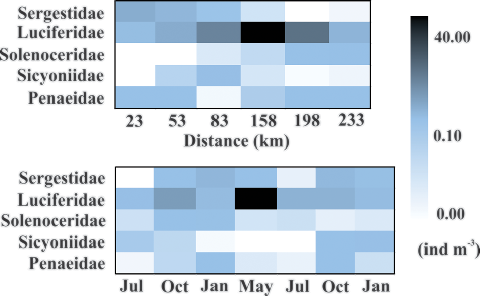
Fig. 5. Heatmap showing the total density distribution (ind m−3) of the dendrobranchiate shrimp assemblage in relation to months and distance from the coast on the Amazon continental shelf (2013–2015).
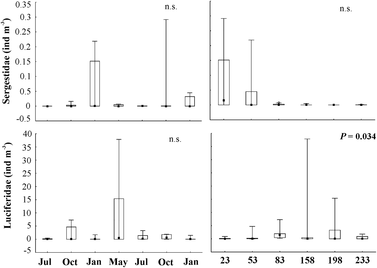
Fig. 6. Minimum and maximum values, medians and 25% and 75% quartiles of density (ind m−3) of sergestoid shrimps considering months and distance from the coast on the Amazon continental shelf (2013–2015). n.s., not significant.
Among luciferid shrimps, Belzebub faxoni was dominant on the ACS, with the highest density both in mysis and in post-larval stages (7580 larvae, mean density: 1.13 ± 3.61 ind m−3) and in juveniles–adults (5454 individuals, 0.80 ± 2.79 ind m−3). Belzebub faxoni was found in all months, and throughout the shelf, whereas Lucifer typus had low densities (28 individuals, 0.08 ind m−3), represented only by juveniles and adults, collected as far as ~190 km from the coast.
Sergestid shrimps were present in all months with lower densities than luciferids. However, they were not present throughout the shelf, having higher densities up to 55 km from the coast (497 individuals; 7.58 ind m−3) and low densities farther than this distance (Figures 5 and 6). A significant decreasing trend (A < 0) was found in the proportion of sergestid shrimps (χ2 = 378.65; P < 0.01) with increased distance from the coast.
Among sergestids, there was predominance of Acetes spp. on the ACS, with the highest densities up to 55 km from the coast (depth ~20 m), where development stages ranging from mysis II to adults were found: mysis II (36 larvae, total density: 0.84 ind m−3), post-larvae (PL) (247 larvae, 3.67 ind m−3), and juveniles–adults (211 individuals, 3.21 ind m−3), including 10 males and 12 females of A. americanus (Figure 5). Sergestes sp. were also found: 1 mysis II and 2 post-larvae (0.02 ind m−3), with low densities collected at the 100-m isobath, starting ~200 km away from the coast.
Distribution of dendrobranchiate shrimp density was significantly correlated with explanatory variables. The RDA model explained ~18% (R 2non-adjusted = 30.74%; F = 2.44; P = 0.001) of the total variation in shrimp assemblages. The two first RDA axes together explained 81.45% of variability; the first axis explained 58.8% of variability and was positively related to salinity (0.78) and negatively related to chlorophyll-a (−0.72). The second axis explained 22.6% of variability and was positively correlated with distance from the coast (0.78) and negatively correlated with temperature (−0.84) (Table 1; Figure 7).

Fig. 7. Representation of the density dispersal of dendrobranchiate shrimps according to explanatory variables on the Amazon continental shelf (2013–2015), produced using Redundancy Analysis (RDA). A: scores of samples with vectors. B: scores of taxa with vectors. Explanation ratio: RDA1: 58.8%; RDA2: 22.6%. Mo.: months, Chlo: chlorophyll-a (μg l−1), T(°C): temperature, Outfw: water outflow, Sal: salinity, DC: distance from the coast (km), My-Lu: Luciferidae mysis, JA-Lu: Luciferidae juveniles and adults, MII-Ac: mysis II of Acetes spp., PL-Ac: post-larvae of Acetes spp., JA-Ac: juveniles and adults of Acetes spp., MIII-So: mysis III of Solenoceridae, MIII-Si: mysis III of Sicyoniidae, MIII-Pe: mysis III of Penaeidae, PL-Pe: post-larvae of Penaeidae.
Table 1. Coefficients of correlation resulting from the Redundancy Analysis (RDA) between explanatory variables and densities of dendrobranchiate shrimp families on the Amazon continental shelf (2013–2015)
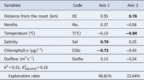
Values in bold indicate correlations higher than 0.7.
Among sergestoid shrimps, Acetes spp. were negatively correlated with chlorophyll-a and Luciferidae were positively correlated with the temporal variable (month), both on axis 1. On axis 2, Acetes spp. was also negatively correlated with temperature (Figure 7, Supplementary Table S2).
Abundance and distribution of penaeoid shrimps
Penaeoid shrimps represented only 3.62% of the total individuals collected on the ACS; however, they were very frequent (76%). They were represented by Solenoceridae (infrequent: 33%), Sicyoniidae and Penaeidae (frequent: 40 and 57%, respectively). All three families had low densities, and Sicyoniidae shrimps had the highest mean density (0.52 ind m−3).
Larvae of sicyoniid shrimps were represented by few specimens (total: 304 larvae), with higher density in phases MI and MII of the mysis stage (239 mysis larvae, total density: 0.62 ind m−3) compared with post-larvae. Sicyoniidae density peaked in January 2015 in the onset of the rainy season (262 individuals, 0.52 ind m−3) and this family was not present in May and July 2014 (peak river discharge). Regarding distribution on the ACS, Sicyoniidae was present only offshore, beyond 50 km, with higher density 83 km away from the coast (282 individuals; 0.64 ind m−3, Figures 5 and 8) and a significant decreasing trend in the frequency of occurrence with increased distance from the coast (A < 0; χ2 = 15.41; P < 0.01).
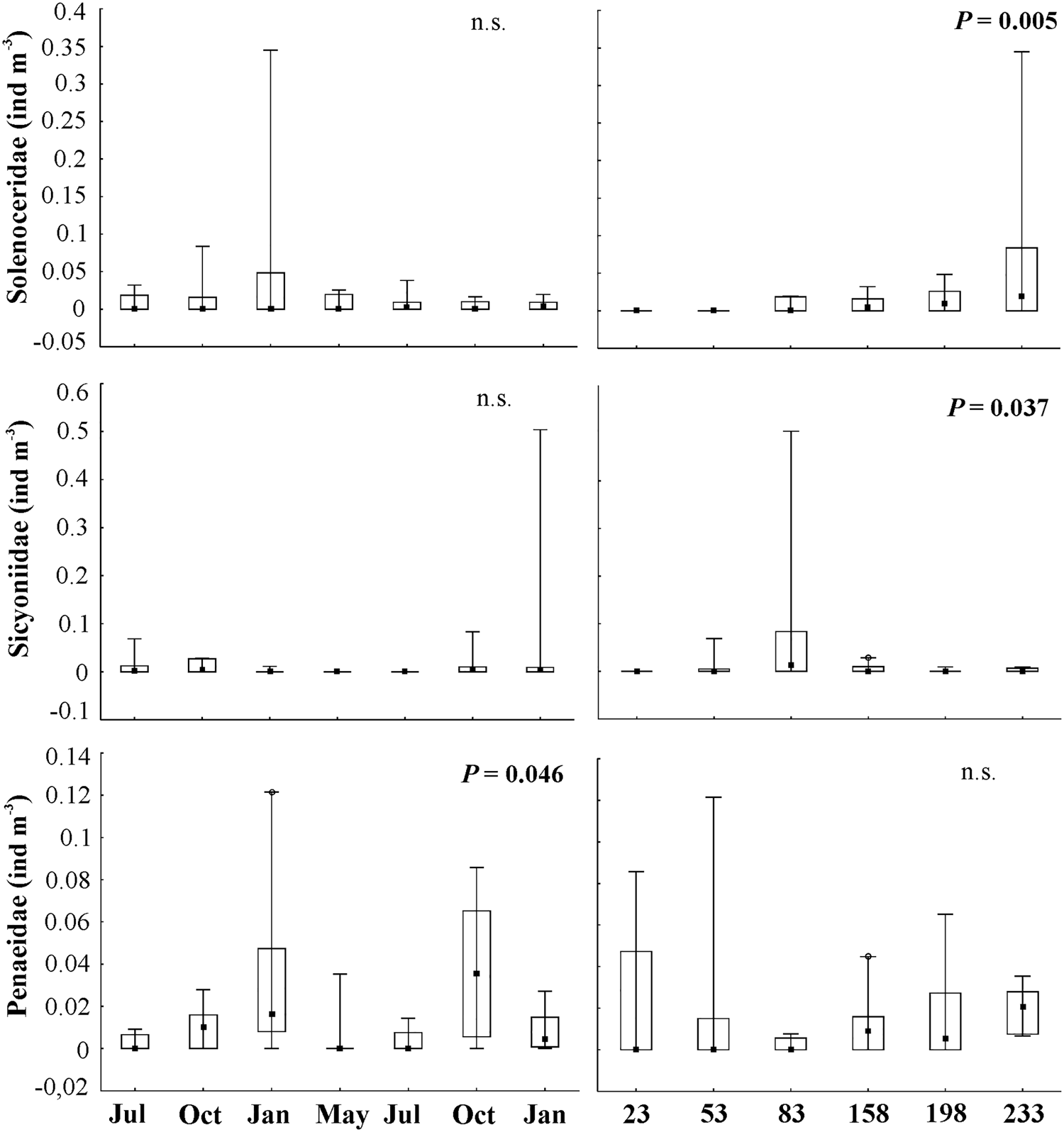
Fig. 8. Minimum and maximum values, medians and 25% and 75% quartiles of density (ind m−3) of penaeoid shrimps considering months and distance from the coast on the Amazon Continental Shelf (2013–2015). n.s., not significant.
Few solenocerid shrimps were found on the shelf (N = 115 larvae) and most were in the mysis III stage (88 larvae, 0.58 ind m−3). Mysis II stages were absent in July 2013 and post-larvae were present only in October 2013 (4 larvae, 0.02 ind m−3). Overall, solenocerid shrimps were present in all months, with the highest density in the onset of the rainy season in January 2014 (39 larvae, 0.40 ind m−3). Solenoceridae was present only farther than 80 km from the coast, with higher densities as far as 200 km (74 individuals; 0.49 ind m−3) (Figures 5 and 8), and a significant increasing trend in the frequency of occurrence on the ACS with increased distance from the coast (A > 0; χ2 = 63.50; P < 0.01).
Penaeid shrimp densities were homogeneous (90 individuals; 0.62 ind m−3), with higher densities of mysis stages compared with post-larvae (53 mysis, 0.51 ind m−3). They were present in all months, with higher density in the dry season, October 2014 (0.22 ind m−3), which was related to the low Amazon River outflow (Z = −3.23; P = 0.001). Penaeidae were present throughout the shelf (Figures 5 and 8), with a significant increasing trend in the frequency of occurrence (A > 0; χ2 = 12.74; P < 0.01) with increased distance from the coast.
Density distribution of penaeoid shrimps was significantly correlated with the explanatory variables in the RDA model; however, few taxa had correlations higher than 0.1 with the RDA axes. Therefore, solenocerid and penaeid mysis III stages were positively correlated with distance from the coast on axis 2 (Figure 7, Supplementary Table S2).
Discussion
This study provides novel information on density distribution of dendrobranchiate shrimps (superfamilies Sergestoidea and Penaeoidea) in the plankton of the Amazon Continental Shelf, with information on seasonal variations, thus helping to pave the way to understanding this large-scale, hugely relevant ecosystem that remains poorly studied. The hypothesis that the distribution of shrimps groups on the ACS is heterogeneous was accepted, and this study revealed different migratory patterns depending on groups, and different tolerances to salinity variations. Previous studies on planktonic shrimps in this region have been based on one single cruise only and analysis were performed to luciferid species (Melo et al., Reference Melo, Neumann-Leitão, Gusmão, Martins-Neto and Palheta2014) and mainly by families (Santana et al., Reference Santana, Lira, Varona, Neumann-Leitão, Araujo and Schwamborn2020), not distinguishing the groups as presented here. Thus, this is the first study to reveal the temporal variability of these key organisms on the ACS (see summarized data in Supplementary Table S1).
In tropical coastal areas, the zooplankton species diversity increases towards outer shelf and open ocean waters (Boltovskoy et al., Reference Boltovskoy, Gibbons, Hutchings, Binet and Boltovskoy1999; Lopes et al., Reference Lopes, Katsuragawa, Dias, Montú, Muelbert, Gorri and Brandini2006). In ACS, an effect of the Amazon river plume is a local drop in the diversity of most oceanic planktonic groups (Boltovskoy et al., Reference Boltovskoy, Gibbons, Hutchings, Binet and Boltovskoy1999), due to the dominance of an immense low-salinity plume (<20) from the inner shelf to mid-shelf areas, as also shown by Santana et al. (Reference Santana, Lira, Varona, Neumann-Leitão, Araujo and Schwamborn2020) who found that the major contributions of marine holopelagic decapods (e.g. penaeid shrimps) occurred in the oceanic area without plume influence.
Aside from reflecting the environmental requirements of each family, the different patterns among shrimps also reflect the complexity of the ACS environment. During our study, the low-salinity plume reached as far as 200 km from the shore, in May. All other months had a more restricted plume (less than ~100 km from the shore), and this allowed observation of shrimp assemblage distribution both at sites under direct influence of the Amazon plume and at sites with more oceanic characteristics.
We observed higher frequency and abundance of Sergestoidea in areas under the influence of the Amazon River plume. Planktonic shrimps densities obtained in this study were similar to those in the Arvoredo Archipelago (Koettker & Freire, Reference Koettker and Freire2006), and São Tomé Cape to Brazil (Brandão et al., Reference Brandão, Garcia and Freire2015). The only study that covered a large extent in the western tropical Atlantic influenced by the Amazon River plume was Santana et al. (Reference Santana, Lira, Varona, Neumann-Leitão, Araujo and Schwamborn2020), who reported the huge abundance of planktonic decapods, mostly Brachyura larvae and luciferids shrimps in coastal and oceanic areas under the influence of the plume of the Amazon River.
The sergestoid shrimp stages that were present ranged from larvae to adults, with emphasis on the high density of B. faxoni, which along with Acetes spp. plays an important role in the food web and produces high biomass in continental shelf environments (Longhurst, Reference Longhurst1985). The holoplanktonic shrimp Lucifer typus was confirmed as an oceanic tropical water shrimp (Bowman & McCain, Reference Bowman and McCain1967; Xu, Reference Xu2010; Melo et al., Reference Melo, Neumann-Leitão, Gusmão, Martins-Neto and Palheta2014; Marafon-Almeida et al., Reference Marafon-Almeida, Pereira and Fernandes2016) while B. faxoni proved to be typically coastal, with the highest densities among all the shrimp taxa in this study (Bowman & McCain, Reference Bowman and McCain1967; Longhurst, Reference Longhurst1985; Arshad et al., Reference Arshad, Ara, Amin, Effendi, Zaidi and Mazlan2011), thus corroborating Melo et al. (Reference Melo, Neumann-Leitão, Gusmão, Martins-Neto and Palheta2014), who reported its high-density pattern on the ACS.
The positive correlation of Luciferidae with months was associated with the dynamics of the Amazon River outflow and salinity on the ACS. This indicates that Luciferidae shrimps, dominated by B. faxoni, were associated with the shortest distance from the coast and highest outflow, which is corroborated by their high densities on the inner-mid shelf (<150 km, present study) and the high abundance of luciferid in the coastal and oceanic areas under Amazon river plume influence seen by Santana et al. (Reference Santana, Lira, Varona, Neumann-Leitão, Araujo and Schwamborn2020). They appear to have a continuous recruitment, with a peak that might be associated with species reproductive and spawning periods (Fugimura et al., Reference Fugimura, Oshiro and Silva2005; Cavalcante-Braga, Reference Cavalcante-Braga2017 unpublished); however, this aspect needs to be further investigated on the ACS.
Among Sergestidae, Sergestes sp. seems to be an oceanic tropical water species (≥36), as is Neosergestes edwardsi (previously Sergestes edwardsi), which has been a good indicator of these water masses (Brandão et al., Reference Brandão, Koettker and Freire2013). On the other hand, Acetes spp. was found to be a coastal species with its entire life cycle occurring in the inner part of the ACS. Two species of the genus Acetes might occur on the ACS: A. americanus, which is distributed on the continental shelf of Brazil and is likely associated with coastal water masses, and A. marinus, which does not have a known larval development and is endemic to the influence area of the Amazon River mouth (D'Incao & Martins, Reference D'Incao and Martins2000; Vereshchaka et al., Reference Vereshchaka, Lunina and Olesen2015). Due to the difficulty in differentiating between the larval stages of these two species, it was not possible to determine if they are concurrent or if they have different distributions on the ACS.
Seasonality of congeners of Acetes spp. is well known; however, this was not evident on the ACS. Overall, recruitment is continuous throughout the year in tropical and subtropical regions, with spawning peaks occurring during hotter seasons (Xiao & Greenwood, Reference Xiao and Greenwood1993; Simões et al., Reference Simões, D'Incao, Fransozo, Castilho and Costa2013a, Reference Simões, Castilho, Fransozo, Negreiros-Fransozo and Costa2013b; Santos et al., Reference Santos, Simões, Bochini, Costa and Costa2015). Acetes spp. distribution was primarily associated with higher temperatures and chlorophyll-a. Acetes americanus is known to have higher abundance in the months with high chlorophyll-a concentration (Santos et al., Reference Santos, Simões, Bochini, Costa and Costa2015) and it occurs in shallower sites with high temperatures and lower salinity values (Simões et al., Reference Simões, Castilho, Fransozo, Negreiros-Fransozo and Costa2013b); these patterns are similar to those found for Acetes spp. on ACS.
Penaeoid larvae were less abundant and were represented by Solenoceridae, Sicyoniidae and Penaeidae. With little variation, all larval stages were present, from mysis I to post-larva, which is in line with the reproductive behaviour of the benthic adult population. Penaeoid distribution might be explained by different factors; this taxon had the highest number of species recorded on the ACS (Barros & Pimentel, Reference Barros and Pimentel2001; Silva et al., Reference Silva, Muniz, Ramos-Porto, Viana and Cintra2002a, Reference Silva, Ramos-Porto, Cintra, Muniz and Silva2002b, Reference Silva, Cintra, Ramos-Porto, Viana, Abrunhosa and Cruz2020), and is expected to have a wider niche. Its low larval density can be explained by different migratory movements (see Dall et al., Reference Dall, Hill, Rothlisberg, Sharples, Blaxter and Southward1990, who identified four patterns for penaeid shrimps' life cycle). It is also likely that penaeoid larval densities reflect diel migrations, especially post-larvae that tend to concentrate at deeper levels during the day, while moving towards the surface at night (Gomez-Ponce & Gracia, Reference Gomez-Ponce and Gracia2003, Reference Gomez-Ponce and Gracia2007, Reference Gomez-Ponce and Gracia2008). Solenocera larvae tend to remain in the middle of the water column, while Sicyonia larvae have wider dispersal in the column and Penaeidae tend to concentrate near the surface between 0 and 10 m depth (Gomez-Ponce & Gracia, Reference Gomez-Ponce and Gracia2008). Efforts should be taken for vertical sampling on the PCA at different depths, to throw some light on this issue.
Solenoceridae species inhabit deeper layers (>80 m), and their reproduction occurs on the outer shelf (Dall et al., Reference Dall, Hill, Rothlisberg, Sharples, Blaxter and Southward1990; Gomez-Ponce & Gracia, Reference Gomez-Ponce and Gracia2003). In previous studies, mysis stages of Solenocera spp. were usually found from mid- to outer shelf (Gomez-Ponce & Gracia, Reference Gomez-Ponce and Gracia2003, Reference Gomez-Ponce and Gracia2007). In the present study, solenocerid larvae were found at mid- to outer shelf stations, as well; this explains the correlation found with distance on the ACS and reflects the reproductive behaviour of adults.
Larval distribution of sicyoniid shrimps occurs from mid- to inner ACS since larval stages of Sicyonia spp. predominated on the ACS ~80 km from the coast. Sicyoniid shrimp adults are usually distributed on the continental shelf at sites deeper than 200 m (D'Incao, Reference D'Incao1995). Sicyonia dorsalis, S. laevigata and S. parri reproduction is known to be continuous, with variable juvenile recruitment and two to three peaks a year, one of which occurs with higher intensity (Bauer & Rivera-Vega, Reference Bauer and Rivera-Vega1992; Castilho et al., Reference Castilho, Furlan, Costa and Fransozo2008). Sicyoniidae larvae was not strongly correlated with any explanatory variable addressed in this study. There is little information available on Sicyoniidae and studies on S. dorsalis and S. typica larvae, which are species that occur on the ACS, are non-existent. According to Costa et al. (Reference Costa, Fransozo and Negreiros-Fransozo2005), S. dorsalis occurs in areas with salinity values above 30. Although the larvae found here on the ACS were not identified at the species level, all of them were found in saline waters.
Penaeidae occurrence was homogeneous throughout the ACS, ranging from mysis to post-larvae; this has also been observed for their counterparts in other regions of the world (Price et al., Reference Price, Mathews, Ingles and Al-Rasheed1993; Rogers et al., Reference Rogers, Shaw, Herke and Blanchet1993; Vance et al., Reference Vance, Haywood, Heales and Staples1996, Reference Vance, Haywood, Heales, Kenyon and Loneragan1998; Castilho et al., Reference Castilho, Furlan, Costa and Fransozo2008; Galindo-Bect et al., Reference Galindo-Bect, Hernández-Ayón, Lavín, Diaz, Hinojosa and Zavala2010; Pham et al., Reference Pham, Charmantier, Wabete, Boulo, Broutoi, Mailliez, Peignon and Charmantier-Daures2012). Penaeid shrimp larvae distribution on ACS was associated with high salinity, and consequently, these larvae are located further from the coast, which proves the hypothesis of higher occurrence far from the plume. The highest penaeid larvae densities occur in the periods with the lowest Amazon River outflow, thus reflecting seasonality from October to January, which is also related with migratory behaviour (e.g. Farfantepenaeus subtilis, according to Aragão et al., Reference Aragão, Silva and Cintra2015). The continuous presence of penaeid larvae in all sampling months and at all sites throughout the ACS proves the importance of this area as a nursery habitat for these shrimps, where juveniles and adults have been captured every year since the 1960s.
This study has shown that the Amazon River outflow has a great influence on the dynamics of Amazon continental shelf salinity and chlorophyll-a, thus explaining shrimp assemblage distribution, as is expected in large river plumes (Dagg et al., Reference Dagg, Benner, Lohrenz and Lawrence2004; Santos et al., Reference Santos, Muniz, Barros-Neto and Araujo2008; Goes et al., Reference Goes, Gomes, Chekalyuk, Carpenter, Montoya, Coles, Yager, Berelson, Capone, Foster, Steinberg, Subramaniam and Hafez2014; Conroy et al., Reference Conroy, Steinberg, Stukel, Goes and Coles2016). Overall, the highest densities occurred nearer the coast, which reinforces the presence of species that endure high variations in environmental factors on the ACS. Our data suggest that Acetes spp. (Sergestidae) is strongly affected by higher temperatures and chlorophyll-a, and B. faxoni shrimps (Luciferidae) are associated with shorter distance and higher outflow. On the other hand, Solenoceridae and Penaeidae distribution is explained by a larger distance from the coast and high salinity.
In conclusion, the planktonic shrimps on the inner shelf were associated with chlorophyll-a, temperature and outflow, and shrimps on the mid-outer shelf were related to salinity and distance from the coast. This study shows information on the distribution of density of Dendrobranchiata shrimps on the Amazon continental shelf for the first time, with a seasonal approach over two years, and helps to pave the way towards characterizing the distribution of these shrimps in a wide area which has been poorly studied so far, serving as a base for future comparisons. Finally, it is worth noting that the Amazon continental shelf is an extremely high priority conservation area as it serves as a nursery and growth area for at least five shrimp families.
Supplementary material
The supplementary material for this article can be found at https://doi.org/10.1017/S0025315421000308
Acknowledgements
The authors are grateful to all researchers and students who participated in the expeditions to the ACS, as well as all students who helped with larval screening. We are also thankful to Professors Dr Nuno F.A.C. Melo and Dr Eduardo Paes (Instituto Sócio-Ambiental e Recursos Hídricos, Universidade Federal Rural da Amazônia) for providing logistical support to the field expeditions. We also appreciate the suggestions of the anonymous referee who improved this work and Mrs Daniela Tannus in reviewing the manuscript.
Financial support
This study was carried out with funding from the National Institute on Science and Technology in Tropical Marine Environments – INCT-AmbTropic by Conselho Nacional de Desenvolvimento Científico e Tecnológico – CNPq (grant number 565054/2010-4) (INCT AmbTropic: https://www.inctambtropicii.org/gt-2-2). This study was also supported by Coordenação de Aperfeiçoamento de Pessoal de Nível Superior – CAPES, Finance Code 001; Fundação Amazônia de Amparo a Estudos e Pesquisas – FAPESPA and PAPQ-FADESP/PROPESP-UFPA for supporting the English version of the manuscript.


