2. Equations and scaling

The non-hydrostatic Boussinesq equations are

(2.1a)\begin{gather} \frac{\partial\boldsymbol{v}}{\partial{t}} + {\boldsymbol{f}} \times \boldsymbol{v} + \boldsymbol{\nabla} p + \boldsymbol{v} \boldsymbol{\cdot} \boldsymbol{\nabla} \boldsymbol{v} + w \frac{\partial\boldsymbol{v}}{\partial{z}} = 0, \end{gather}

(2.1b)\begin{gather}\frac{\partial{w}}{\partial{t}} + \frac{\partial{p}}{\partial{z}} - b + \boldsymbol{v} \boldsymbol{\cdot} \boldsymbol{\nabla} w + w \frac{\partial{w}}{\partial{z}} = 0, \end{gather}

(2.1c)\begin{gather}\frac{\partial{b}}{\partial{t}} + N^2 w + \boldsymbol{v} \boldsymbol{\cdot} \boldsymbol{\nabla} b + w \frac{\partial{b}}{\partial{z}} = 0, \end{gather}

(2.1d)\begin{gather}\boldsymbol{\nabla} \boldsymbol{\cdot} \boldsymbol{v} + \frac{\partial{w}}{\partial{z}} =0, \end{gather}

where $\boldsymbol {v} = u \boldsymbol {\hat {x}} + v \boldsymbol {\hat {y}}$ is the horizontal velocity, $w$ is the vertical velocity, $b$ is the buoyancy, $N$ is the constant Buoyancy frequency, $\boldsymbol {f} = f \boldsymbol {\hat {z}}$ with $f$ being the constant inertial frequency and $\boldsymbol {\nabla } = \boldsymbol {\hat {x}} \partial /\partial x + \boldsymbol {\hat {y}} \partial /\partial y$.

We non-dimensionalize (2.1) using the scaling

(2.2)\begin{equation} \left.\begin{gathered}t \rightarrow t/f, \quad \boldsymbol{x} \rightarrow L \boldsymbol{x}, \quad z \rightarrow H z, \quad \boldsymbol{v} \rightarrow U \boldsymbol{v}, \quad w \rightarrow (H U/L) w, \\ p \rightarrow (fUL) p, \quad b \rightarrow (fUL/H) b. \end{gathered}\right\} \end{equation}

In the above, time, $t$, was scaled using the inertial frequency $f$. Horizontal and vertical length scales, $L$ and $H$, may be thought of as the breadth and depth of the domain. Horizontal velocity was scaled using an arbitrary velocity scale, $U$, and accordingly the scale for vertical velocity, $HU/L$, was chosen to satisfy the continuity equation, (2.1d). The scale for pressure was chosen by requiring that the horizontal pressure gradient ($\boldsymbol {\nabla } p$) balanced the Coriolis term ($\boldsymbol {f} \times \boldsymbol {v}$). Finally, balancing the vertical pressure gradient ($\partial p/ \partial z$) with buoyancy gave us the scale for buoyancy.

Using (2.2) to non-dimensionalize (2.1) gives us

(2.3a)\begin{gather} \frac{\partial{\boldsymbol{v}}}{\partial{t}} + {\boldsymbol{\hat{z}}} \times \boldsymbol{v} + \boldsymbol{\nabla} p + Ro \left( \boldsymbol{v} \boldsymbol{\cdot} \boldsymbol{\nabla} \boldsymbol{v} + w \frac{\partial{\boldsymbol{v}}}{\partial{z}} \right) = 0, \end{gather}

(2.3b)\begin{gather}\frac{\partial{w}}{\partial{t}} + \alpha^2 \left( \frac{\partial{p}}{\partial{z}} - b \right) + Ro \left( \boldsymbol{v} \boldsymbol{\cdot} \boldsymbol{\nabla} w + w \frac{\partial{w}}{\partial{z}} \right) = 0, \end{gather}

(2.3c)\begin{gather}\frac{\partial{b}}{\partial{t}} + w + Ro \left( \boldsymbol{v} \boldsymbol{\cdot} \boldsymbol{\nabla} b + w \frac{\partial{b}}{\partial{z}} \right) = 0, \end{gather}

(2.3d)\begin{gather}\boldsymbol{\nabla} \boldsymbol{\cdot}\boldsymbol{v} + \frac{\partial{w}}{\partial{z}} =0, \end{gather}

where $Ro=U/fL$ is the Rossby number and $\alpha =N/f$. We also set $L = N H /f$ ($N H /f$ being the deformation scale) so that the Froude number $Fr = U/NH = U/fL = Ro$. Our scaling therefore ensures that we are in the parameter regime $Ro = Fr$, or in other words, the Burger number, $Bu = (Ro/Fr)^2 = 1$. This means that on setting $Ro \ll 1$ in the system (2.3), we also obtain $Fr \ll 1$, ensuring that we are in the rapidly rotating and strongly stratified parameter regime. In this work we will investigate wave–balance interactions in the $Ro \sim Fr \ll 1$ regime.

We obtain the following linear equations by setting $Ro=0$ in (2.3):

(2.4a)\begin{gather} \frac{\partial{\boldsymbol{v}}}{\partial{t}} + {\boldsymbol{\hat{z}}} \times \boldsymbol{v} + \boldsymbol{\nabla} p = 0, \end{gather}

(2.4b)\begin{gather}\frac{\partial{w}}{\partial{t}} + \alpha^2 \left( \frac{\partial{p}}{\partial{z}} - b \right) = 0, \end{gather}

(2.4c)\begin{gather}\frac{\partial{b}}{\partial{t}} + w = 0, \end{gather}

(2.4d)\begin{gather}\boldsymbol{\nabla} \boldsymbol{\cdot} \boldsymbol{v} + \frac{\partial{w}}{\partial{z}} =0. \end{gather}

The solutions of the linear equations can be decomposed into waves and a balanced flow field. The geostrophic balanced component, denoted with subscript ‘$G$’ hereafter, does not evolve at the linear level and is governed by the equations

(2.5a)\begin{gather} \boldsymbol{\hat{z}} \times {{{\boldsymbol{v}}}_{\scriptscriptstyle{G}}} + \boldsymbol{\nabla} {{{{p}}_{\scriptscriptstyle{G}}}} = 0, \end{gather}

(2.5b)\begin{gather}\frac{\partial{{{{{p}}_{\scriptscriptstyle{G}}}}}}{\partial{z}} - {{{{b}}_{\scriptscriptstyle{G}}}} = 0, \end{gather}

(2.5c)\begin{gather}{{{{w}}_{\scriptscriptstyle{G}}}}=0, \end{gather}

(2.5d)\begin{gather}\boldsymbol{\nabla} \boldsymbol{\cdot} {{{ \boldsymbol{v}}}_{\scriptscriptstyle{G}}} =0, \end{gather}

while the internal gravity wave field, denoted with subscript ‘$W$’ hereafter, evolves according to

(2.6a)\begin{gather} \frac{\partial{ {{{ \boldsymbol{v}}}_{\scriptscriptstyle{W}}} }}{\partial{t}} + {\boldsymbol{\hat{z}}} \times {{{ \boldsymbol{v}}}_{\scriptscriptstyle{W}}} + \boldsymbol{\nabla} {{{{p}}_{\scriptscriptstyle{W}}}} = 0, \end{gather}

(2.6b)\begin{gather}\frac{\partial{{{{w}}_{\scriptscriptstyle{W}}}}}{\partial{t}} + \alpha^2 \left( \frac{\partial{{{{p}}_{\scriptscriptstyle{W}}}}}{\partial{z}} - {{{{b}}_{\scriptscriptstyle{W}}}} \right) = 0, \end{gather}

(2.6c)\begin{gather}\frac{\partial{{{{b}}_{\scriptscriptstyle{W}}}}}{\partial{t}} + {{{{w}}_{\scriptscriptstyle{W}}}} = 0, \end{gather}

(2.6d)\begin{gather}\boldsymbol{\nabla} \boldsymbol{\cdot} {{{ \boldsymbol{v}}}_{\scriptscriptstyle{W}}} + \frac{\partial{{{{w}}_{\scriptscriptstyle{W}}}}}{\partial{z}} =0. \end{gather}

Throughout this work we will use above wave–balance decomposition, allowing us to decompose the flow into linear internal gravity waves and a geostrophically balanced component. The above wave–balance decomposition is orthogonal, implying that the total energy is the exact sum of the energies of the two fields with no cross-terms, i.e. $E={{{{E}}_{\scriptscriptstyle {G}}}} + {{{{E}}_{\scriptscriptstyle {W}}}}$, where $E$, ${{{{E}}_{\scriptscriptstyle {G}}}}$ and ${{{{E}}_{\scriptscriptstyle {W}}}}$ denote total, balanced and wave energies, respectively. The unambiguous nature of above decomposition has resulted in it being applied to multiple oceanographic data sets, atmospheric data sets and idealized geophysical turbulent simulation data sets (Bartello Reference Bartello1995; Smith & Waleffe Reference Smith and Waleffe2002; Bühler et al. Reference Bühler, Callies and Ferrari2014; Callies, Ferrari & Bühler Reference Callies, Ferrari and Bühler2014; Hernandez-Duenas, Smith & Stechmann Reference Hernandez-Duenas, Smith and Stechmann2014; Herbert et al. Reference Herbert, Marino, Rosenberg and Pouquet2016; Rocha et al. Reference Rocha, Chereskin, Gille and Menemenlis2016; Lien & Sanford Reference Lien and Sanford2019, for example). In this paper we will examine how a broad spectrum of internal gravity waves affects the dynamics of the geostrophic balanced flow in different balance-to-wave energy regimes.

3. Numerical experiments

To explore wave–balance interactions in different regimes we numerically integrated (2.3) in the domain $(x,y,z) \in [0, 2 {\rm \pi}] \times [0, 2 {\rm \pi}] \times [-{\rm \pi} , 0]$ with periodic boundary conditions in the $x$ and $y$ directions and with rigid lids on top ($z=0$) and bottom ($z=-{\rm \pi}$). The simulations were performed using a dealiased pseudospectral code with $384^3$ grid points and fourth-order Runge–Kutta scheme for time integration. Hyperdissipation terms of the form $\nu \varDelta _{3D}^8 \boldsymbol {v}$, $\nu \varDelta _{3D}^8 w$ and $\nu \varDelta _{3D}^8 b$, where $\varDelta _{3D}= \partial ^2/\partial x^2 + \partial ^2/\partial y^2 + \partial ^2/\partial z^2$, were added to (2.3a), (2.3b) and (2.3c). We chose hyperviscosity $\nu = 10^{-34}$, providing us with a wide range of inviscid scales and ensuring that dissipation was confined to grid scale. Numerical convergence was ensured by examining successive simulations with half the time step used in the previous simulation, until the solutions and statistics were seen to remain unchanged with further decrease in time step.

We initialized (2.3) with wave and balanced flow at low wavenumbers and waited until the initial transients settled and turbulence was fully developed (we refer the reader to the Appendix for a detailed description of the initialization procedure). Such fully developed turbulent flows were the starting point (i.e. $t=0$) of all of our diagnoses. We performed a wide range of experiments by varying initial balanced and wave energy levels, and based on our exploratory experiments we first examine two specific regimes in great detail and then briefly discuss the changes in neighbouring regimes. The two regimes we explore in detail first will be the comparable wave (CW) regime with ${({{{{E}}_{\scriptscriptstyle {G}}}}/{{{{E}}_{\scriptscriptstyle {W}}}})}_{t=0} \sim O(1)$, where wave and balanced energies are comparable in strength, and strong wave (SW) regime with ${({{{{E}}_{\scriptscriptstyle {G}}}}/{{{{E}}_{\scriptscriptstyle {W}}}})}_{t=0} \sim O(Ro^2)$, where wave energy significantly exceeds balanced energy. We used $\alpha =20$ and $Ro=0.1$ for the numerical experiments reported below.

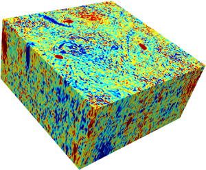
On exploring the flow in the two regimes, the geostrophic flow in the CW regime was seen to organize into large-scale coherent vortices, a snapshot being shown in figure 1(a). In contrast, the geostrophic vorticity in the SW regime consists of small-scale structures and shows no sign of large-scale coherent vortices, as can be seen in figure 1(b). Figure 2(a, b) shows the geostrophic and wave energy spectra at $t=15\,000$ on two different horizontal planes – a quarter and three-quarters below the top surface. In our freely evolving experiments, although the spectral slopes were seen to fluctuate a little over the duration of the experiments (see caption of figure 2), the qualitative features were seen to be similar at different times. Specifically, a persistent feature of the geostrophic spectra is the presence of a shallower inertial range in the SW regime (black curves in figure 2a) when compared with the CW regime (red curves in figure 2a). The formation of small-scale features in the geostrophic flow seen in figure 1(b) leads to relatively higher geostrophic energy at small scales, which eventually get dissipated.

Figure 1. Geostrophic vorticity, ${{{{\zeta }}_{\scriptscriptstyle {G}}}}$, in (a) CW and (b) SW regimes at $t=15\,000$. To highlight flow features in the interior, the above panels show a horizontal slice of the domain with $z=-{\rm \pi} /4$ being the top surface and $z=-{\rm \pi}$ being the bottom surface.

Figure 2. (a) Geostrophic and (b) wave horizontal energy spectra at $t=15\,000$ on the plane $z=-{\rm \pi} /4$ (continuous curves) and $z=-3{\rm \pi} /4$ (dashed curves). During the course of the experiments, the wave spectrum was seen to fluctuate between $k_h^{-1.7}$ and $k_h^{-1.9}$ in CW and SW regimes. The geostrophic spectrum in the CW regime varied between $k_h^{-3.2}$ and $k_h^{-3.9}$. In the SW regime the geostrophic spectrum varied between $k_h^{-1.9}$ and $k_h^{-2.1}$. Notice that the geostrophic energy spectrum is shallower in the SW regime when compared with the CW regime, indicating the higher geostrophic energy content at small scales. All the spectral slopes were calculated based on a best fit in the range $k_h \in [10, 70]$. Straight lines corresponding to $k_h^{-2}$ and $k_h^{-3}$ are given on the above spectral plots for reference.

We will now examine energy exchanges between waves and geostrophic balanced flow. On applying the wave–balance decomposition to the governing equations (2.3), including hyperdissipative terms, we obtain the energy change equations for wave and balanced components at each wavenumber $(k_x, k_y, k_z)$ (see Thomas & Daniel (Reference Thomas and Daniel2020) for the detailed procedure). Integrating over angles in spectral space gives us triadic energy equations for balanced flow and wave field as a function of total wavenumber $k = \sqrt {k_x^2 + k_y^2 + k_z^2}$ as follows:

(3.1a)\begin{align} \frac{\partial{ \hat{E}_{G} (k) }}{\partial{t}} &= T_{GGG}(k) + T_{GWW} (k) + T_{GGW} (k) - \hat{D}_{G} (k) , \end{align}

(3.1b)\begin{align}\frac{\partial{ \hat{E}_{W} (k) }}{\partial{t}} &= T_{WWW} (k) + T_{WGW} (k) + T_{WGG} (k) - \hat{D}_{W} (k). \end{align}

The left-hand sides of (3.1) give the rate of change of balance and wave energy at wavenumber $k$, while the right-hand sides of the above equations contain the triadic interaction terms responsible for the changes, such as balance-only triads ($T_{GGG}$), balance–wave–wave triads ($T_{GWW}$), balance–balance–wave triads ($T_{GGW}$), and so on. Each triadic term $T_{ABC} (k)$ above indicates the net effect the modes $B$ and $C$ have on mode $A$ at wavenumber $k$. The dissipation terms are indicated by $\hat {D}$.

On summing (3.1) from $k=0$ to the maximum resolved wavenumber, $k_{{max}}$, and time-integrating the equations so obtained from an arbitrary time $t=t_0$ to $t=t$, we get wave–balance energy change equations

(3.2a)\begin{align} {{{E}}_{\scriptscriptstyle{G}}} (t) - {{{E}}_{\scriptscriptstyle{G}}} (t_0) &= \underbrace{ E_{GWW} (t) + E_{GGW} (t) }_{ E_G^{{triads}} (t)} - {{{D}}_{\scriptscriptstyle{G}}} (t) , \end{align}

(3.2b)\begin{align}{{{E}}_{\scriptscriptstyle{W}}} (t) - {{{E}}_{\scriptscriptstyle{W}}} (t_0) &= \underbrace{ E_{WGW} (t) + E_{WGG} (t) }_{ E_W^{{triads}} (t)} - {{{D}}_{\scriptscriptstyle{W}}} (t). \end{align}

Since triadic interaction of specific kinds must conserve energy, we have $E_{GWW} (t) + E_{WGW} (t) = 0$ and $E_{GGW} (t) + E_{WGG} (t) = 0$, which leads to $E_G^{{triads}} (t)+ E_W^{{triads}} (t)=0$; i.e. nonlinear energy exchange between waves and geostrophic flow must be conservative – a loss in wave energy must be accompanied by a gain in geostrophic energy and vice versa. For pure geostrophic triads and pure wave triads, we have $E_{GGG}(t) = E_{WWW} (t) = 0$, since geostrophic triads by themselves are incapable of changing net geostrophic energy and wave triads by themselves are incapable of changing net wave energy. Consequently, $E_{GGG}$ and $E_{WWW}$ terms do not appear in (3.2).

On examining wave–balance energy transfers based on (3.2), we found no noticeable energy exchange in the CW regime. In contrast, significant energy exchanges were observed in the SW regime and energy transfers during a certain time interval in the SW regime are given in figure 3. As seen in figure 3(a), two-way wave–balance energy exchanges take place, this being a generic feature of the SW regime. Waves gain energy from and lose energy to the balanced flow. Figure 3(a) also reveals the conservation of energy transfer under triadic interactions noted earlier, i.e. $E_G^{{triads}} (t)+ E_W^{{triads}} (t)=0$. On examining the contribution of different triadic terms, energy transfers are seen to be primarily due to the triads $E_{GWW}$ and $E_{WGW}$, while transfers due to $E_{WGG}$ and $E_{GGW}$ triads were much weaker. This behaviour can be seen in figure 3(b) showing the changes in the different triadic components during the same time interval as figure 3(a).

Figure 3. (a) Time evolution of $E_G^{{triads}}$ and $E_W^{{triads}}$. (b) Time evolution of different triadic components in (3.2). In above plots $t_0=15\,000$.

We follow up the net energy transfers with an examination of the spectral energy fluxes. On summing (3.1) from $k_{{max}}$ to $k$, we obtain the energy flux equations for balanced and wave components as

(3.3a)\begin{align} \frac{\partial{ \hat{\hat{E}}_{\scriptscriptstyle{G} } (k, t) }}{\partial{t}} &= \underbrace{ \varPi_{\scriptscriptstyle {GGG} }(k, t) + \varPi_{\scriptscriptstyle {GWW} } (k, t) + \varPi_{\scriptscriptstyle {GGW} } (k, t) }_{\varPi_{\scriptscriptstyle {G} }} - \hat {\hat D}_{\scriptscriptstyle {G} } (k, t) , \end{align}

(3.3b)\begin{align}\frac{\partial{ \hat{\hat{E}}_{\scriptscriptstyle{W} } (k, t) }}{\partial{t}} &= \underbrace{ \varPi_{\scriptscriptstyle {WWW} } (k, t) + \varPi_{\scriptscriptstyle {WGW} } (k, t) + \varPi_{\scriptscriptstyle {WGG} } (k, t) }_{\varPi_{\scriptscriptstyle {W} }} - \hat{\hat{D}}_{\scriptscriptstyle {W} } (k, t), \end{align}

where $\hat {\hat {E}}_{\scriptscriptstyle {G} } (k, t)$ and $\hat {\hat {E}}_{\scriptscriptstyle {W} } (k, t)$ represent the energy contained in the spectral band $[k, k_{\text {max}}]$ for balanced flow and waves, while $\varPi _{\scriptscriptstyle {G} }$ and $\varPi _{\scriptscriptstyle {W} }$ represent spectral fluxes of balanced and wave energy. Similar to the decomposition implemented in (3.1), the spectral fluxes are further decomposed into different triadic contributions above. The triadic flux terms satisfy

(3.4a)\begin{gather} \varPi_{\scriptscriptstyle {GGG} }(k=0, t) =0, \end{gather}

(3.4b)\begin{gather}\varPi_{\scriptscriptstyle {WWW} }(k=0, t) = 0, \end{gather}

(3.4c)\begin{gather}\varPi_{\scriptscriptstyle {GWW} } (k=0, t) + \varPi_{\scriptscriptstyle {WGW} } (k=0, t) = 0 , \end{gather}

(3.4d)\begin{gather}\varPi_{\scriptscriptstyle {GGW} } (k=0, t) + \varPi_{\scriptscriptstyle {WGG} } (k=0, t) = 0. \end{gather}

Figure 4(a–d) shows the waves’ and geostrophic fluxes and their decomposition for CW and SW regimes, respectively. The spectral fluxes were computed using (3.3) and time-averaged in the interval $15\,000-\delta \leqslant t \leqslant 15\,000 + \delta$. We set $\delta$ to be a few eddy turnover time scales based on multiple iterative experiments, ensuring that $\delta$ was large enough to remove short time scale transient fluctuations from the spectral fluxes, while also making sure that the time interval of averaging was small enough so that the magnitudes of spectral fluxes did not change significantly during the averaging window. In both CW and SW regimes, waves were seen to exhibit a forward energy flux with $\varPi _W >0$. In the CW regime, balanced flow was seen to catalyze the forward flux of wave energy at all times, in addition to triadic wave interactions, similar to the findings discussed in connection to freely evolving simulations in Bartello (Reference Bartello1995) (observe that $\varPi _{WGW}$ is comparable or higher in magnitude than $\varPi _{WWW}$ in the range $k \sim 10\text {--}100$ in figure 4a). For the SW regime shown in figure 4(c), we find that although $\varPi _{WGW}$ is still positive, $\varPi _{WWW}$ is the dominant contributor towards waves’ spectral fluxes.

Figure 4. Spectral flux of the wave and geostrophic flow field and its decomposition into constituents computed based on (3.3) at $t=15\,000$ for (a,b) CW ((a) ${{{{\varPi }}_{\scriptscriptstyle {W}}}}$, (b) ${{{{\varPi }}_{\scriptscriptstyle {G}}}}$); and (c,d) SW ((c) ${{{{\varPi }}_{\scriptscriptstyle {W}}}}$, (d) ${{{{\varPi }}_{\scriptscriptstyle {G}}}}$) regimes.

Complementary to the waves’ energy flux, figures 4(b) and 4(d) show the spectral fluxes of the geostrophic flow for CW and SW cases, respectively. Notice that in the CW regime (figure 4b) $\varPi _G$ is negative with almost entire contribution being from $\varPi _{GGG}$. The geostrophic flow exhibits an inverse energy flux, with balanced triadic interactions ($G-G-G$) playing the dominant role, similar to that seen in quasi-geostrophic turbulence phenomenology (McWilliams Reference McWilliams1989; Smith & Vallis Reference Smith and Vallis2001; Nadiga Reference Nadiga2014). Contrary to the CW case, figure 4(d) shows that $\varPi _G$ is predominantly positive in the SW regime. Although $\varPi _{GGG}$ is still fully negative in this regime, $\varPi _{GWW}$ is positive and of relatively larger magnitude, resulting in positive valued $\varPi _G$ for $k \sim 10\text {--}100$. Waves therefore facilitate a forward flux of geostrophic energy in the SW regime. Although the flux plots shown in figure 4 correspond to a specific time ($t=15\,000$) and are subject to minor changes in the quantitative values, the qualitative features we glean from figure 4 were seen to be maintained at all times that we examined. Specifically, the inviscid range of scales of the balanced flow in the SW regime were seen to be qualitatively similar to that shown in figure 4(d), characterized by a forward energy flux with positive $\varPi _G$, resulting in enhanced dissipation of balanced energy. Therefore, as the waves flux energy downscale in the SW regime, they facilitate the transfer of geostrophic energy from large inviscid scales to small dissipative scales.

Figure 5(a) shows the fractional change in geostrophic energy in CW and SW regimes. The forward energy flux leads to dissipation of the geostrophic flow, resulting in a gradual drop in geostrophic energy with time, as shown by the black curve in figure 5(a). By the end of the experiment at $t=25\,000$, the geostrophic energy drops by 47 %. In the CW regime on the other hand, where an inverse geostrophic energy flux leads to the formation of large-scale coherent vortices, we observed only 0.65 % drop in geostrophic energy by $t=25\,000$. Figure 5(b) shows the time series of the ratio of geostrophic and wave energy in the SW regime. Since both geostrophic and wave energy decrease in the SW regime, the balance-to-wave energy ratio remains $O(Ro^2)$ at all times. Therefore, although our experiments were freely evolving, the SW regime with ${{{{E}}_{\scriptscriptstyle {G}}}}/ {{{{E}}_{\scriptscriptstyle {W}}}} \sim Ro^2$ was maintained throughout the evolution of the system.

Figure 5. Panel (a) shows the fractional change in geostrophic energy in CW and SW regimes. The inset shows a magnified plot of the drop in geostrophic energy in the CW regime. Panel (b) shows the time series of ${{{{E}}_{\scriptscriptstyle {G}}}}/{{{{E}}_{\scriptscriptstyle {W}}}}$ for the SW regime. On averaging the time series given in panel (b) from $t=0$ to $t=25\,000$, we obtained the mean balance-to-wave-energy ratio as $\overline {({{{{E}}_{\scriptscriptstyle {G}}}}/{{{{E}}_{\scriptscriptstyle {W}}}})} = 0.0124 = 1.24 Ro^2$.

3.1. A detailed examination of the wave and the balanced field

So far all our analysis was based on the wave–balance decomposition given in (2.6) and (2.5). In the weakly nonlinear regimes we are based in, with $Ro \ll 1$, this decomposition gives us a geostrophic balanced component and an orthogonal component – internal gravity waves. In all the regimes discussed in this paper the wave field was seen to be primarily linear, based on a detailed examination of the waves’ frequency spectra. An example set for the SW regime is shown in figure 6. Observe that the low and intermediate wavenumbers (figures 6a and 6b), which contain higher energy content, exhibit more linear behaviour with the frequencies obtained numerically (red curves) being peaked at the linear wave frequencies at those wavenumbers based on the dispersion relationship (dashed black lines), whereas higher wavenumbers with lesser energy content show much more spread across frequencies (figure 6c). The departure from linear wave dynamics is expected at small scales with lower wave energy levels where the dynamics are strongly nonlinear. At such small scales, especially close to dissipative scales, although the wave–balance decomposition formally provides us a ‘wave’ component, this component does not correspond to linear waves. Consequently, our results described earlier, comparing the CW and SW regimes with the same geostrophic energy level but different wave energy levels, point out that in the SW regime linear waves facilitate the transfer of geostrophic energy from large weakly nonlinear scales to smaller strongly nonlinear scales and from thereon toward dissipative scales. If wave energy is not high enough (as in the CW regime), such a large-to-small scale transfer of geostrophic energy would not take place.

Figure 6. Shown above is an example set of frequency spectra of wave velocity, ${{{\hat {u}}}_{\scriptscriptstyle {W}}}(k_h, k_z)$, in the SW regime for (a) low (b) intermediate and (c) high wavenumbers. The discontinuous black curves show the linear internal gravity wave frequency at corresponding wavenumbers. The frequency spectra were computed using time series of different wavenumbers from $t=15\,000\text {--}15\,500$.

We next examine the frequency spectra of the balanced flow. Unlike the CW regime where the wave and balanced fields have similar magnitudes, the SW regime is characterized by linear wave fields being an order of magnitude stronger than the balanced flow field so that nonlinear wave–wave interaction terms are of the same strength as the balanced field. Consequently, the balanced flow is heavily influenced by waves in the SW regime, resulting in high frequency fluctuations in the geostrophic flow. To extract a slow balanced component from the total balanced flow, we performed a running time averaging operation on the balanced fields as

(3.5)\begin{equation} {{{\bar u}}_{\scriptscriptstyle{G}}} (\boldsymbol{x}, z, t; \tau) = (1/ \tau) \int_{t-\tau/2}^{t+\tau/2} {{{{{u}}_{\scriptscriptstyle{G}}}}} (\boldsymbol{x}, z, s) \,\textrm{d} s, \end{equation}

where $\tau$, the averaging time interval, is several inertial wave periods. Figure 7(a) shows the frequency spectra of the balanced velocity ${{{{{u}}_{\scriptscriptstyle {G}}}}}$ before (black curve) and after (red curve) the fast-time-averaging operation with $\tau =25$, i.e. approximately four inertial wave periods. Observe that time averaging removes high frequency fluctuations from the frequency spectrum, providing us a slow-balanced field. We computed the slow geostrophic flow energy (using ${{{\bar u}}_{\scriptscriptstyle {G}}}$, ${{{\bar v}}_{\scriptscriptstyle {G}}}$ and ${{{\bar b}}_{\scriptscriptstyle {G}}}$) and compared it with the original unaveraged geostrophic energy (computed using ${{{u}}_{\scriptscriptstyle {G}}}$, ${{{{v}}_{\scriptscriptstyle {G}}}}$ and ${{{{b}}_{\scriptscriptstyle {G}}}}$) during multiple time intervals. An example comparison is given in figure 7(b), with the black curve showing the evolution of the original balanced energy (i.e. a part of the black curve shown in figure 5a) and the red curve showing the evolution of the slow-balanced energy. The good agreement between the curves in figure 7(b) points out that the decrease in the balanced energy seen in figure 5(a) corresponds to a decrease in the slow-evolving geostrophic balanced flow's energy. Although fast fluctuations are inherently present in the geostrophic flow in the SW regime, their effects are overall weak.

Figure 7. (a) Frequency spectra of ${{{{{u}}_{\scriptscriptstyle {G}}}}}$ (black curve) and ${{{\bar u}}_{\scriptscriptstyle {G}}}$ (red curve). (b) The black curve shows geostrophic energy computed using the balanced fields, this being a small portion of the black curve shown in figure 5(a). The red curve shows the change in slow balanced energy, computed based on the slow balanced fields: ${{{\bar u}}_{\scriptscriptstyle {G}}}$, ${{{\bar v}}_{\scriptscriptstyle {G}}}$ and ${{{\bar b}}_{\scriptscriptstyle {G}}}$.

3.2. Comparison with other works

We will now compare our results in the SW regime with two other works. The first one is that of Wagner & Young (Reference Wagner and Young2015). Within the framework of the hydrostatic Boussinesq equations Wagner & Young (Reference Wagner and Young2015), operating in the same SW regime as ours, used asymptotic analysis to derive an evolution equation for the potential vorticity anomaly (or available potential vorticity as they identify it), $Q = (N^2 \hat{\boldsymbol{z}} + \boldsymbol{\nabla}_{3D}b)\boldsymbol{\cdot}(\,f \hat{\boldsymbol{z}} + \boldsymbol{\nabla}_{3D} \times \boldsymbol{v})- f\,N^2$, where $\boldsymbol{\nabla}_{3D} = \hat{\boldsymbol{x}}\partial/\partial x + \hat{\boldsymbol{y}}\partial/\partial y+ \hat{\boldsymbol{z}}\partial/\partial z$, as

(3.6)\begin{equation} \frac{\partial{Q_{{sw}}}}{\partial{t}} + \partial [ \psi_{{sw} }, Q_{{sw}}] = 0, \end{equation}

with $Q_{{sw}} = \varDelta_{3D} \psi _{{sw} } + q_{{waves}}$, $q_{waves}$ being the contribution due to quadratic time-averaged wave–wave interactions alone (see (4.52)–(4.55) in Wagner & Young (Reference Wagner and Young2015)). In the above, $\partial [\, f , g] = f_x g_y - f_y g_x$ is the Jacobean and $\psi _{{sw} }$ is the stream function corresponding to the Lagrangian averaged balanced flow, which also contains nonlinear wave–wave interactions (see their (4.38)).

Multiple assumptions are required to derive approximate asymptotic models such as (3.6). These include the assumption of hydrostatic balance for the internal gravity wave field, completely ignoring near-resonant interactions, and the usage of asymptotic analysis that relies on a fast time scale, corresponding to the time scale of waves, and a slow time scale, corresponding to the slow eddy turnover time scale. Formally, such an asymptotic analysis with two distinct time scales is expected to hold only for a few eddy turnover time scales. In addition to the above-mentioned assumptions and restrictions, Wagner & Young (Reference Wagner and Young2015) assume that quadratic nonlinear wave–wave interaction terms evolve on the same time scale as the mean flow. This specific assumption is key to their analysis using two distinct asymptotic time scales. Consequently, Wagner & Young (Reference Wagner and Young2015) end up with a Lagrangian mean flow that is in geostrophic balance, i.e. Lagrangian mean flow is completely determined by the stream function $\psi _{{sw} }$ in their formalism. Such geostrophically balanced Lagrangian mean flows apply for special cases alone, since the Lagrangian mean flow can have significant unbalanced component (see examples and discussions in Thomas, Bühler & Smith (Reference Thomas, Bühler and Smith2018)).

In spite of the assumptions and restrictions stated above, (3.6) is still a useful approximate model capable of providing qualitative insight into the wave-dominant SW regime. Equation (3.6) is basically an asymptotic recasting of the potential vorticity equation, the key result being that the potential vorticity field and the asymptotically approximate balanced stream function ($\psi _{{sw} }$) is composed of a slow Eulerian component and wave–wave interaction terms, i.e. nonlinear wave interactions form a part of the balanced flow in the SW regime. From our numerical experiment in the SW regime, for an illustration, figure 8 shows the potential vorticity anomaly at $t=15\,000$. Observe the ubiquitous presence of small-scale features, similar to the geostrophic vorticity field shown in figure 1(b), emphasizing the role of high energy waves on balanced dynamics. In the SW regime Wagner & Young (Reference Wagner and Young2015) define the balanced field to be the flow field associated with the Lagrangian mean flow, corresponding to $\psi _{{sw}}$, which contains an Eulerian mean component and quadratic wave–wave interaction terms. As mentioned earlier, the asymptotic formulation they implement enforces the Lagrangian mean flow to be in geostrophic balance, a result that does not hold in general. Nevertheless, the main take-home message here is that balanced flow is significantly affected by waves in SW regimes. Since both wave and balanced flow fields were seen to exhibit a forward energy flux in the SW regime based on our linear wave-Eulerian geostrophic balance decomposition, and given that the materially advected potential vorticity field is composed of fine-scale structures that get dissipated at small scales (recall figure 8), qualitatively similar results should be expected – i.e. a forward flux of wave and balanced energy – if an alternate flow decomposition, such as one that might involve the Lagrangian mean flow, is implemented.

Figure 8. Non-dimensional form of $Q = (N^2 \hat{\boldsymbol{z}} + \boldsymbol{\nabla}_{3D} b)\boldsymbol {\cdot}(\, f \hat{\boldsymbol{z}} + \boldsymbol{\nabla}_{3D} \times \boldsymbol {v} )- f\kern0.4pt N^2$ (potential vorticity anomaly) at $t=15\,000$ in the SW regime.

The second recent study that is useful to examine here is that of Barkan et al. (Reference Barkan, Winters and McWilliams2017), where a fast–slow decomposition of the fields were used, similar to the Leonard decomposition implemented in large eddy simulations (see Sagaut (Reference Sagaut2005) for specific examples). Although the fast–slow decomposition of Barkan et al. (Reference Barkan, Winters and McWilliams2017) does not rely on asymptotic approximations, the time-averaged field constitutes a slow field and is not generically in geostrophic balance, making the definition of balance ambiguous. Barkan et al. (Reference Barkan, Winters and McWilliams2017), operating in the $Ro \sim 1$ regime (contrary to the $Ro \ll 1$ regime we are based in), report results from a regime with 90 % of the flow energy being in fast component and rest in slow component. In their wave-dominant regime, Barkan et al. (Reference Barkan, Winters and McWilliams2017) report that coherent structures were seen to be severely disrupted, along with significant fast–slow energy exchanges. Furthermore, Barkan et al. (Reference Barkan, Winters and McWilliams2017) report fast waves facilitating a transfer of slow energy from large mesoscales to small submesoscales, a phenomenology that is similar to what we observe in our SW regime – waves facilitating a forward flux of geostrophic energy.

Above discussion connecting our results with that of Wagner & Young (Reference Wagner and Young2015) and Barkan et al. (Reference Barkan, Winters and McWilliams2017), in spite of differences in the detailed set-ups in these works, bring out several key features of SW regimes. Internal waves and balanced flow are inseparably intertwined in the SW regime. Small-scale formation in the balanced flow, significant wave–balance energy exchanges and enhanced dissipation of geostrophic energy are the norm in wave-dominant regimes, these features being the exact opposite of the phenomenology seen in quasi-geostrophic turbulence that is devoid of waves. The comparisons discussed above emphasize that irrespective of the specific kind of flow decomposition used, qualitatively similar phenomenology must be expected in wave-dominant regimes in general.

3.3. An illustrative experiment

To further elucidate the role of high energy waves on balanced dynamics, we will now consider a special experiment. Recall the SW regime we examined so far and the energy change in the geostrophic flow given in figure 5(a). In figure 9 we show this SW case again, with the black curve, this being the same black curve in figure 5(a), showing the drop in geostrophic energy with time. Suppose we removed all the waves in the system at a specific time, say $t=10\,000$. We do so by applying the wave–balance decomposition given in (2.6) and (2.5) and instantaneously setting the wave component of the solution to zero, and continuing integration of the governing equations. In this case the system at $t=10\,000$ is filtered of all waves and is left to evolve with a geostrophic balanced component alone. The blue curve in figure 9 shows the changes in geostrophic energy on integrating the Boussinesq equations after removal of waves at $t=10\,000$ – observe that there is no noticeable change in geostrophic energy on removing waves. The balanced flow, in the absence of high energy waves, evolves with insignificant energy loss.

Figure 9. An experiment illustrating the effect of high energy waves on the geostrophic balanced flow. The black curve above is the same black curve as that shown in figure 5(a). The blue curve above shows the geostrophic energy change following the removal of waves at $t=10\,000$.

Of course, we note that the above experiment described in connection to figure 9 is highly contrived, especially since we are unable to rationalize the possibility of a realistic physical process instantaneously annihilating all the waves in the system at a specific time ($t=10\,000$). Nevertheless, the experiment and a comparison between the black and the blue curves starting at $t=10\,000$ in figure 9 helps drive the main idea home: the dynamics of the geostrophic flow differs substantially in the presence of high energy waves. High energy waves interact with the geostrophic flow, facilitating its dissipation. If wave energy is not high enough, the geostrophic flow evolves unaffected by waves with negligible energy loss. The significant changes high energy waves can induce in the dynamics of balanced flow, as specifically highlighted with our illustrative experiment in figure 9, is the main result of this study.

3.4. Neighbouring parameter regimes

So far we examined a specific SW regime with ${{{{E}}_{\scriptscriptstyle {G}}}}(0) = 4.75 \times 10^{-2}$, ${{{{E}}_{\scriptscriptstyle {W}}}}(0) =3.49$ leading to ${{{{E}}_{\scriptscriptstyle {G}}}}(0)/{{{{E}}_{\scriptscriptstyle {W}}}}(0) =1.36Ro^2$ in great detail. In this case, as mentioned in connection with figure 5(b), we obtained a mean balance-to-wave energy ratio of $\overline {({{{{E}}_{\scriptscriptstyle {G}}}}/{{{{E}}_{\scriptscriptstyle {W}}}})}=1.24Ro^2$ over the duration of the experiment and a net drop in geostrophic energy by 47 %. These details have been summarized as Exp. 1 in table 1. We will now briefly describe the changes seen on varying balanced and wave energy levels within generic SW regimes with $\overline {{{{{E}}_{\scriptscriptstyle {G}}}}/{{{{E}}_{\scriptscriptstyle {W}}}}}\lesssim Ro^2$.

Table 1. Summary of results in SW regimes. Initial geostrophic and wave energies were chosen based on multiple iterative simulations so as to obtain a wide set of ${{{{E}}_{\scriptscriptstyle {G}}}}(0)/{{{{E}}_{\scriptscriptstyle {W}}}}(0)$ values, as given in the fifth column above. All numerical integrations used $Ro=0.1$ and were performed up to $t=25\,000$.

On increasing geostrophic energy (${{{{E}}_{\scriptscriptstyle {G}}}}(0) = 8.31 \times 10^{-2}$) while maintaining a wave energy level close to that in the SW regime (${{{{E}}_{\scriptscriptstyle {W}}}}(0) =3.21$), we were able to obtain a mean balance-to-wave energy ratio $\overline {({{{{E}}_{\scriptscriptstyle {G}}}}/{{{{E}}_{\scriptscriptstyle {W}}}})}=2.73Ro^2$. In this case, identified as the SW$_a$ regime, we observed a 49 % drop in geostrophic energy (slightly higher than that seen in our SW regime), as shown by the red curves in figure 10 and summarized as Exp. 2 in table 1. To examine the effect of a lower balance-to-wave energy ratio, we decreased geostrophic energy (${{{{E}}_{\scriptscriptstyle {G}}}}(0) = 2.81 \times 10^{-2}$), maintaining wave energy level close to earlier values (${{{{{E}}_{\scriptscriptstyle {W}}}}}(0)=3.44$), thereby obtaining $\overline {({{{{E}}_{\scriptscriptstyle {G}}}}/{{{{E}}_{\scriptscriptstyle {W}}}})}=0.79Ro^2$ and a 42 % drop in geostrophic energy by final time (slightly lower than that seen in our SW regime), as can be seen from the blue curves in figure 10 and summarized as Exp. 3 in table 1 with the regime name SW$_b$. To see the effect of a much lower balance-to-wave energy ratio, we further lowered balanced energy (${{{{E}}_{\scriptscriptstyle {G}}}}(0) = 1.19 \times 10^{-2}$) without much change in the wave energy (${{{{E}}_{\scriptscriptstyle {W}}}}(0) =3.52$). In this case, identified as SW$_c$ regime, we obtained a mean energy ratio $\overline {({{{{E}}_{\scriptscriptstyle {G}}}}/{{{{E}}_{\scriptscriptstyle {W}}}})}=3.41Ro^3$ and 32 % drop in geostrophic energy. This is seen in the green curves in figure 10 and is summarized as Exp. 4 in table 1. Finally on increasing both wave and geostrophic initial energies, ${{{{E}}_{\scriptscriptstyle {G}}}}(0) = 7.13\times 10^{-2}$ and ${{{{{E}}_{\scriptscriptstyle {W}}}}}(0) =4.57$ – a case identified as SW$_d$ regime, we obtained a mean energy ratio $\overline {({{{{E}}_{\scriptscriptstyle {G}}}}/{{{{E}}_{\scriptscriptstyle {W}}}})}=1.54Ro^2$ and a 53 % drop in geostrophic energy by final time. This case is shown by black curves in figure 10 and summarized as Exp. 5 in table 1.

Figure 10. (a) Fractional change in geostrophic balanced energy in $\textrm {SW}_a\text {--}\textrm {SW}_d$ regimes. (b) Time series of $({{{{E}}_{\scriptscriptstyle {G}}}}/{{{{E}}_{\scriptscriptstyle {W}}}})$ in $\textrm {SW}_a\text {--}\textrm {SW}_d$ regimes.

Overall, the specific magnitude of change in the geostrophic energy is variable depending on the parameters, as can be gleaned from table 1. Nevertheless, some qualitatively generic features can still be inferred. For a given wave energy level, increasing geostrophic energy accelerates wave–balance interactions and leads to higher drop in geostrophic energy by final time while the opposite holds for decreasing geostrophic energy. This trend can be seen on comparing $\textrm {SW}_a$, $\textrm {SW}_b$ and $\textrm {SW}_c$ regimes in table 1. All three regimes have similar wave energy levels, but decreasing geostrophic energy leads to a lower net drop in geostrophic energy. On a complementary note, for a fixed wave energy level, decreasing balanced energy was seen to reduce the rate of wave energy decay and vice versa on increasing balanced energy. This can be seen by examining the last column of table 1 for $\textrm {SW}_a$, $\textrm {SW}_b$ and $\textrm {SW}_c$ cases. Finally, the SW$_d$ case serves as an example where both balanced and wave energy was increased, resulting in accelerated interactions and a higher drop in balanced and wave energy.

Above described qualitative features are as expected based on the weakly nonlinear equations (2.3), i.e. increasing wave and geostrophic energy accelerates wave–balance interactions and results in higher net energy drops, while decreasing wave and geostrophic energy decelerates the rate of interactions and reduces the net energy drop by final time. We found a similar effect on changing $Ro$. Increasing $Ro$ in (2.3) accelerated wave–balance exchanges while the opposite was observed on decreasing $Ro$. Based on a wide set of experiments we examined by varying balanced and wave energy levels, a selected set of results are presented in table 1 to give an idea of the magnitudes of energy changes in different regimes and thereby informing us about the qualitative trends to be expected on changing energy levels.

Apart from the relative differences in magnitudes of energy changes, all SW regimes characterized by $\overline {({{{{E}}_{\scriptscriptstyle {G}}}}/{{{{E}}_{\scriptscriptstyle {W}}}})} \lesssim Ro^2$ featured qualitatively similar dynamics. Specifically, small-scale features in the geostrophic flow, a forward geostrophic energy flux and significant dissipation of geostrophic flow, leading to a gradual drop in geostrophic energy were observed in SW regimes in general. As pointed out with our contrived yet illustrative experiment in figure 9, SW regimes are characterized by strongly coupled exchanges between waves and balanced flow. In the absence of waves or if wave energy is not significantly higher than balanced energy, balanced flow would evolve completely unaffected by waves and transfer energy to larger scales.

4. Summary and discussion

In this paper we explored interactions between a broad spectrum of internal gravity waves and geostrophic balanced flows in different balance-to-wave energy regimes using numerical integration of the non-hydrostatic Boussinesq equations. The main findings of this work are summarized as schematics in figure 11. In CW regimes with ${{{{E}}_{\scriptscriptstyle {G}}}}/{{{{E}}_{\scriptscriptstyle {W}}}}\sim O(1)$, the geostrophic balanced flow exhibits an inverse energy flux resulting in the formation of domain-sized coherent vortices, while waves undergo a forward energy flux and get dissipated at small scales. Waves and balanced flow do not exchange energy and the balanced flow behaves as if waves were completely absent – similar to balanced flow dynamics in quasi-geostrophic turbulence devoid of waves. In contrast, SW regimes with ${{{{E}}_{\scriptscriptstyle {G}}}}/{{{{E}}_{\scriptscriptstyle {W}}}}\lesssim Ro^2$ are characterized by two-way wave–balance energy exchanges, leading to the formation of small-scale features in the balanced flow. The geostrophic flow is no longer decoupled from waves in SW regimes: the flow is an entanglement of energetically interacting waves and balanced flow. In these regimes, as waves undergo a forward energy flux, they insinuate a forward energy flux for the geostrophic flow. High energy waves can therefore facilitate the transfer of geostrophic energy from large scales, where dynamics are weakly nonlinear, to smaller scales, where strongly nonlinear dynamics take over, and from there onto dissipative scales.

Figure 11. Turbulent energy flow pathways in different parameter regimes. The red and black boxes symbolize internal gravity waves and geostrophic balanced flow fields, respectively. The blue arrow at the bottom indicates that wavenumbers increase to the right. (a) The CW regime. This shows the scenario when waves are comparable in strength to the balanced flow. In such cases, waves undergo a forward energy flux (small red horizontal arrows in the waves’ box) while the balanced flow exhibits an inverse energy flux (small black horizontal arrow in the balanced flow's box). (b) The SW regime. This shows the case of high wave-energy regimes. Both waves and balanced flow undergo forward energy flux in such regimes (small red and black horizontal arrows inside the boxes), accompanied by two-way energy transfer between waves and balanced flow (discontinuous red and black vertical arrows between boxes).

Our study highlights that the turbulent dynamics of the geostrophic balanced flow is sensitive to the amount of wave energy. The presence of high energy waves can trigger a transition in the direction of geostrophic energy flux from inverse to forward, leading to enhanced dissipation of balanced energy. A broad set of transitions in turbulent flows has been identified in physical systems in the past (see for example Alexakis & Biferale (Reference Alexakis and Biferale2018) and Pouquet et al. (Reference Pouquet, Rosenberg, Stawarz and Marino2019) and references therein). Our results demonstrating a reversal in the energy flux directions of the geostrophic balanced energy is an addition, from the geophysical fluid dynamics point of view, to the list physical systems exhibiting a transition in turbulent dynamics.

In hindsight, our findings also reveal ruggedness of the geostrophic balanced flow. Although the quasi-geostrophic equation is formally derived excluding waves, the geostrophic balanced flow evolves unaffected by waves unless wave energy is significantly higher than balanced energy. In other words, features of the geostrophic balanced flow often observed in quasi-geostrophic regimes – such as inverse energy flux and the formation of large-scale coherent vortices – are equally valid in the presence of waves, as long as wave energy is not severely high. From an oceanographic point of view this means that a broad spectrum of internal waves interacting with balanced flow can dissipate balanced energy only if wave energy is significantly higher than balanced energy.

We have summarized in table 2 the energy exchanges between different kinds of waves and balanced flow based on the investigation presented in this work and our former works, Thomas & Yamada (Reference Thomas and Yamada2019), Thomas & Arun (Reference Thomas and Arun2020) and Thomas & Daniel (Reference Thomas and Daniel2020). On investigating energy exchanges between internal tides and balanced flow, Thomas & Yamada (Reference Thomas and Yamada2019) observed no energy exchanges in CW regime, while waves fed balanced energy in SW regimes and lead to an increase in balanced energy with time. The second and third row of table 2 describe this. On examining energetic interactions between near-inertial waves and balanced flow, Thomas & Daniel (Reference Thomas and Daniel2020) found that waves directly extracted energy from balanced flows in CW regimes. Amongst the broad set of wave–balance investigations we undertook, this is the only case where (i) waves directly extracted balanced energy and (ii) significant energy exchanges were observed in CW regime. On exploring SW regimes, Thomas & Daniel (Reference Thomas and Daniel2020) and Thomas & Arun (Reference Thomas and Arun2020) found that near-inertial waves transferred energy to the balanced flow in SW regimes. These results are highlighted in the fourth and fifth rows of table 2. Finally, the present work examined energetic interactions between a broad spectrum of waves and balanced flow. Contrary to our former studies where a specific wave–balance energy transfer direction was unambiguously identified, two-way wave–balance energy exchanges were seen to be the case for the broad spectrum of internal waves examined in this study. The resulting forward flux of geostrophic energy was seen to lead to significant dissipation of geostrophic energy. Therefore a broad spectrum of internal gravity waves can enhance small-scale dissipation of geostrophic energy. The results for a broad spectrum of waves interacting with balanced flow is highlighted in the sixth and seventh rows of table 2.

Table 2. The above table summarizes energetic interactions between different kinds of waves and balanced flows in the small Rossby number regime based on the results from present study, and Thomas & Yamada (Reference Thomas and Yamada2019), Thomas & Arun (Reference Thomas and Arun2020) and Thomas & Daniel (Reference Thomas and Daniel2020).

The results of our series of wave–balance investigations summarized in table 2 indicate that the direction of wave–balance energy transfers is dependent on the kind of wave field and the relative energy levels of the wave and the balanced flow. Depending on the kind of wave field and its energy level, waves may directly extract energy from balanced flow, feed balanced flow, or facilitate transfer of balanced energy from large inviscid scales to small dissipative scales. Given that large-scale ocean models have difficulties in resolving fast waves and small-scale dynamics, development of appropriate parameterizations for internal gravity waves remains an unresolved challenge for the climate-scale ocean modelling community (MacKinnon et al. Reference MacKinnon2017; Whalen et al. Reference Whalen2020). Our detailed investigations focusing on different kinds of wave fields in a wide range of parameter regimes indicate that parameterizations for unresolved fast wave fields must take into account the detailed nature of the wave field and its energy level. We hope that our results will assist in the development of efficient wave parameterizations, beneficial for climate-scale ocean models, in the near future.