


1. Introduction
Taylor–Couette flow occurs between two concentric cylinders, one or both of which is rotating, and has been of interest to the fluids community, rheologists, process engineers and mathematicians over the past century (Taylor Reference Taylor1923; Donnelly Reference Donnelly1991). This is in part motivated by the fact that, in spite of its simple configuration, Taylor–Couette flow of Newtonian fluids can yield a vast array of complex dynamics, including a wide variety of steady and unsteady flow states (Coles Reference Coles1965; Andereck, Liu & Swinney Reference Andereck, Liu and Swinney1986), mode competition (Dutcher & Muller Reference Dutcher and Muller2009), chaos (Akonur & Lueptow Reference Akonur and Lueptow2003) and transition to turbulence (Grossmann, Lohse & Sun Reference Grossmann, Lohse and Sun2016; Gul, Elsinga & Westerweel Reference Gul, Elsinga and Westerweel2018). In the relatively simple case in which the outer cylinder is fixed, the system can be characterised using only the Reynolds number
 \begin{equation} Re = \frac{\rho \omega r_i d}{\mu}, \end{equation}
where  $\rho$ and
  $\mu$ are the fluid density and dynamic viscosity, respectively,
  $\omega$ is the rotation speed,
  $r_i$ are the radius of the inner cylinder, and
  $d$ is the gap between the inner and outer cylinder radii (
 $d = r_o - r_i$). Likewise, the system geometry can be expressed using two non-dimensional groups; the radius ratio,
  $\eta = r_i / r_o$, and the aspect ratio,
  $\varGamma = L/d$, where
  $L$ is the cylinder length. When the Reynolds number is low, the flow is characterised by uniform shear (circular Couette flow, CCF), and at a critical point,
  $Re_c$, the flow becomes unstable and a series of toroidal vortices form along the fluid annulus (Taylor vortex flow, TVF). Further increases in
  $Re$ cause this state in turn to become unstable and undergo oscillations (wavy vortex flow, WVF). If the Reynolds number is increased further, additional frequencies appear, inducing a more complicated unsteady flow (Coughlin & Marcus Reference Coughlin and Marcus1992; Imomoh, Dusting & Balabani Reference Imomoh, Dusting and Balabani2010), until the flow ultimately becomes turbulent. Because of this rich set of dynamic states, Taylor–Couette flow has been widely used as a means to study flow transitions and instabilities (Fardin, Perge & Taberlet Reference Fardin, Perge and Taberlet2014).
This has also served as a motivation to study Taylor–Couette flow of non-Newtonian fluids, as it allows the effects of various rheological parameters on the flow stability to be examined (Muller Reference Muller2008). One of the most common features of non-Newtonian fluids is shear-thinning, which is observed in many polymer solutions (Larson & Desai Reference Larson and Desai2015), cell cultures (Cagney et al. Reference Cagney, Zhang, Bransgrove, Allen and Balabani2017) and particle suspensions (Mueller, Llewellin & Mader Reference Mueller, Llewellin and Mader2010), and is characterised by a viscosity that scales with strain rate,  $\mu \sim \dot {\gamma }^{n-1}$, where
  $\dot {\gamma }$ is strain rate and
  $n$ is the flow index (with
  $n=1$ for Newtonian fluids). This can lead to spatial and temporal variations in viscosity, requiring the use of a reference viscosity to calculate the Reynolds number; in Taylor–Couette flow it is common to define
  $Re$ with respect to the viscosity found at the ‘nominal’ strain rate,
  $\omega r_i / d$.
Several researchers have addressed the effect of shear-thinning on the critical Reynolds number for the formation of Taylor vortices, predicting a decrease in  $Re_c$ with increased shear-thinning for large values of
  $\eta$ (i.e. when curvature effects are small) (Coronado-Matutti, Souza Mendes & Carvalho Reference Coronado-Matutti, Souza Mendes and Carvalho2004; Caton Reference Caton2006; Ashrafi Reference Ashrafi2011), which has been supported by various numerical and experimental studies (Lockett, Richardson & Worraker Reference Lockett, Richardson and Worraker1992; Khali, Nebbali & Bouhadef Reference Khali, Nebbali and Bouhadef2013; Cagney & Balabani Reference Cagney and Balabani2019b). Bahrani et al. (Reference Bahrani, Nouar, Neveu and Becker2015) found that for a very large gap,
  $\eta = 0.4$, shear-thinning led to an increase in the wavelength of Taylor vortex flow (i.e. a decrease in the number of vortices), in agreement with their predictions from linear stability theory. Escudier, Gouldson & Jones (Reference Escudier, Gouldson and Jones1995) also observed an increase in wavelength associated with shear-thinning, and using laser-Doppler velocimetry showed that the non-Newtonian rheology affected the structure of individual vortices, noting an increase in the asymmetry between the strength of the inward and outward jets between vortices. They also found that for the two shear-thinning fluids they examined (aqueous suspensions of xanthan gum and a Laponite/CMC blend, the latter of which was also thixotropic), the vortices exhibited a slow axial drift, which they assumed to be a steady-state process.
Recent work by the current authors (Cagney & Balabani Reference Cagney and Balabani2019a,Reference Cagney and Balabanib), using particle image velocimetry and flow visualisation to study Taylor–Couette flow of xanthan gum solutions, showed that shear-thinning also altered the wavy state, inducing significant variability in the amplitude of the waves along the axis, despite the relatively small aspect ratio,  $\varGamma = 12.97$. With increased shear-thinning, the spacing of vortices became increasingly irregular as
  $Re$ increased, similar to the drift noted by Escudier et al. (Reference Escudier, Gouldson and Jones1995), suggesting that as well as increasing the global wavelength of the flow, shear-thinning caused the wavelength to become more variable along the cylinder axis. The wavelength was also found to change as
  $Re$ was slowly increased, via the sudden creation and destruction of vortices (Cagney & Balabani Reference Cagney and Balabani2019a). Such transitions have been noted in previous studies of Taylor–Couette flow of Newtonian fluids and are associated with the wavy instability, which leads to an expansion of vortices near the centre of the flow cell and a squeezing of vortices near the ends, until the squeezed vortices are ultimately destroyed via merger with their neighbours (Park & Crawford Reference Park and Crawford1982; Crawford, Park & Donnelly Reference Crawford, Park and Donnelly1985). Beavers & Joseph (Reference Beavers and Joseph1974) also reported the merger of vortices in a solution of polyacrlyamide (PAA) in glycerol–water as the Reynolds number was increased, which they found to be strongly hysteretic, but they did not present information on the rheology of their fluid.
While several researchers have commented on the lack of experimental data on Taylor–Couette flow of shear-thinning fluids (Escudier et al. Reference Escudier, Gouldson and Jones1995; Coronado-Matutti et al. Reference Coronado-Matutti, Souza Mendes and Carvalho2004; Ashrafi Reference Ashrafi2011; Alibenyahia et al. Reference Alibenyahia, Lemaitre, Nouar and Ait-Messaoudene2012), by comparison there has been extensive work in recent decades examining Taylor–Couette flow of viscoelastic fluids. In this case, as well as inertial and viscous forces, the fluids are affected by elastic forces, typically due to dispersed polymers. This requires an additional non-dimensional group, the Deborah number,  $De = \lambda _r \dot {\gamma }$ (which in this context is equivalent to the Weissenberg number (Schäfer, Morozov & Wagner Reference Schäfer, Morozov and Wagner2018)), where
  $\lambda _r$ is the relaxation time of the fluid. The relative importance of viscoelasticity in Taylor–Couette flow is often expressed using the ratio of the Deborah and Reynolds number,
  $De/Re$ (Groisman & Steinberg Reference Groisman and Steinberg1998; Latrache et al. Reference Latrache, Abcha, Crumeyrolle and Mutabazi2016), referred to as the elasticity number.
Early studies showed that the addition of a small amount of polymers led to an increase in the critical Reynolds number (Rubin & Elata Reference Rubin and Elata1966; Denn & Roisman Reference Denn and Roisman1969), but as Muller (Reference Muller2008) notes, the relevance of many early studies is limited due to incomplete rheological characterisation of the fluids. Several more recent studies have examined the dynamics of viscoelastic fluids with negligible shear-thinning (Boger fluids). For dilute suspensions with very weak elasticity,  $De/Re \leq 0.023$, the elasticity has a non-monotonic effect on the critical Reynolds numbers for various flow regimes, but these do not differ significantly from those seen in the Newtonian case (Dutcher & Muller Reference Dutcher and Muller2011). At slightly higher elasticity,
  $De/Re \gtrsim 0.1$, the flow transitions from circular Couette flow to an unsteady state, characterised by standing waves (Groisman & Steinberg Reference Groisman and Steinberg1996; Baumert & Muller Reference Baumert and Muller1999; Dutcher & Muller Reference Dutcher and Muller2013), ‘disordered oscillations’ (Groisman & Steinberg Reference Groisman and Steinberg1996, Reference Groisman and Steinberg1997), elastic turbulence (Liu & Khomami Reference Liu and Khomami2013) or ‘spiral’ or ‘ribbon’ states (Thomas et al. Reference Thomas, Al-Mubaiyadh, Sureshkumar and Khomami2006; Latrache et al. Reference Latrache, Abcha, Crumeyrolle and Mutabazi2016). At higher values of
  $De/Re$, a purely elastic instability occurs, which is independent of Reynolds number (Groisman & Steinberg Reference Groisman and Steinberg1998) and is characterised by isolated vortex pairs called ‘diwhirls’ (Groisman & Steinberg Reference Groisman and Steinberg1997; Kumar & Graham Reference Kumar and Graham2000; Lange & Eckhardt Reference Lange and Eckhardt2001).
Most polymer solutions that are not very dilute or have a highly viscous suspending medium will exhibit both shear-thinning and viscoelasticity (Larson Reference Larson1992). Larson (Reference Larson1989) modelled Taylor–Couette flow of a Doi–Edwards fluid (viscoelastic and strongly shear-thinning) and found that while the viscoelasticity has a non-monotonic effect on the critical Reynolds number, shear-thinning was always destabilising. This observation was supported by the experimental studies of Yi & Kim (Reference Yi and Kim1997), who examined the stability of ultra-dilute solutions of PAA, polyacrylic acid and xanthan gum, and Crumeyrolle & Mutabazi (Reference Crumeyrolle and Mutabazi2002), who measured the stability of aqueous solutions of polyethyleneoxide (PEO). Crumeyrolle and Mutabazi found that for dilute concentrations,  $c < 500\ \textrm {ppm}$, the flow exhibited the same progression of states as a Newtonian fluid (
 $\textrm {CCF}\rightarrow \textrm {TVF} \rightarrow \textrm {WVF}$), but for
  $c > 500\ \textrm {ppm}$, they found that the flow transitioned to a standing wave, which was attributed to an increase in elasticity. However, it should be noted that the relaxation time was inferred from the flow curves, rather than being estimated directly from dynamic rheological tests, and, therefore, the elasticity values may not be reliable.
It is clear that there is a lack of experimental data on Taylor–Couette flow of fluids that are both shear-thinning and viscoelastic. Specifically, it remains unclear how the flow states change as  $Re$ is increased for shear-thinning, viscoelastic fluids, what rheological factors control these transitions, how vortex drift and sudden changes in the wavelength are affected by the fluid rheology and how repeatable and deterministic these processes are. In order to address these questions, we present flow visualisation measurements of Taylor–Couette flow for a series of solutions of xanthan gum in a glycerol–water solvent, spanning the inelastic (
 $De \ll 1$), weakly viscoelastic (
 $De/Re \ll 1$) and viscoelastic (
 $De/Re > 0.1$) regimes. The remainder of the paper is structured as follows; details of our experimental system and the rheological characterisation of the polymer solutions are presented in § 2; the results are discussed in § 3, with specific emphasis on the wavy instability, the splitting and merger of vortices, and the axial drift; additional data is presented in § 4 to confirm that the novel phenomena observed are independent of the acceleration rate of the cylinder; and finally some concluding remarks are made in § 5.
2. Experimental details
The experiments were performed in a specially designed Taylor–Couette flow cell, which was comprised of a thin acrylic pipe as the outer cylinder, mounted vertically between two acrylic plates, and a nylon inner cylinder, which was spray-painted black to reduce reflections. The inner and outer radii of the flow cell were 21.66 mm and 27.92 mm, respectively, and it had an axial length of  $L = 155\ \textrm {mm}$, yielding a radius ratio of
  $\eta = 0.77$ and an aspect ratio of
  $\varGamma = 21.56$. The top acrylic plate was sealed to ensure that a no-slip condition existed at both the top and bottom of the flow cell, i.e. there was no free surface.
The flow cell was surrounded by a rectangular chamber in which water was recirculated via a temperature bath to ensure that the temperature remained constant at  $20\,^{\circ }\textrm {C}$ throughout experiments. The temperature within the flow cell was measured immediately before and after each experiment, and it was found to vary by less than
  $0.2\,^{\circ }\textrm {C}$, with a variation of less than
  $0.1\,^{\circ }\textrm {C}$ (i.e. the resolution of the temperature sensor) for the vast majority of cases.
The inner cylinder was connected to the drive shaft of a stepper motor (Smart Drive Ltd.), the rotation of which was monitored using an optical encoder with a resolution of 2000 pulses per revolution, such that the cylinder speed could be controlled to a high degree of precision.
Experiments were performed using a mixture of three parts deionised water and one part glycerol, with various quantities of xanthan gum (Sigma Aldrich) ranging from 0 to 2000 ppm, as listed in table 1. Gel permeation chromatography was used to characterise the xanthan molecules, which were found to have a mean molecular weight of  $M_w = 1.76 \times 10^6\ \textrm {g} \ \textrm {mol}^{-1}$ and a polydispersity of 1.1. A rotary mixer (Silverson) was used to ensure that the polymer was uniformly dispersed throughout the fluid. The shear rheology of each fluid was measured three times using a rotational rheometer (ARES, TA Instruments) and a cup and bob geometry. The flow curves for each fluid are presented in figure 1. The shear rheology could be well described using the Carreau model,
 \begin{equation} \mu\left(\dot{\gamma} \right) = \mu_{\infty} + \left( \mu_0 - \mu_{\infty} \right) \left( 1 + \left( \lambda_c \dot{\gamma} \right)^2 \right)^{\left(({n - 1})/{2}\right)}, \end{equation}
where  $\mu _{\infty }$ and
  $\mu _0$ are the viscosity values at infinite and zero shear, respectively,
  $\lambda _c$ is the characteristic time scale and
  $n$ is the flow index. The estimated Carreau parameters for each fluid are listed in table 1.
Table 1. Rheological properties of each of the solutions of xanthan gum in glycerol–water studied. The mean effective flow index,  $\overline {n_e}$, is obtained by averaging the value of
  $n_e$ (2.3) found over the range
  $Re = 50\text {--}1000$. The suspension regime is characterised based on the trends in
  $\mu _0$,
  $\lambda _c$ and
  $\lambda _r$, as shown in figure 3.


Figure 1. Variation in the measured viscosity with strain rate for each of the eight fluids examined, with varying concentrations of xanthan gum. The lines represent the best fit to the Carreau model, with the various Carreau parameters listed in table 1. Data points where the measured stress was less than 0.02 Pa were neglected.
In order to characterise the viscoelastic properties of each fluid, the storage and loss moduli ( $G'$ and
  $G''$, respectively) were measured using oscillatory shear tests, with a peak strain of 5 %, which prior tests indicated was well within the linear viscoelastic regime. Figure 2 summarises the variations in the storage and loss moduli with oscillation frequency for each polymer suspension. Elasticity can be said to dominate the rheology when the storage modulus exceeds the loss modulus, i.e. when
  $G' \geq G''$. The oscillation frequency at which this crossover occurs,
  $\omega _r$, can be used to define the relaxation time of the fluid,
  $\lambda _r = 2 {\rm \pi}/ \omega _r$. These values are found using figure 2 and are listed in table 1. For dilute concentrations,
  $c < 100\ \textrm {ppm}$,
  $G'$ does not exceed
  $G''$ over the range of oscillation frequencies accessible in the rheometer (up to
  $100\ \textrm {rad} \ \textrm {s}^{-1}$), which implies a relaxation time of
  $\lambda _r \ll 0.063\ \textrm {s}$.

Figure 2. Variation in the storage ( $G'$) and loss (
 $G''$) moduli with oscillations frequency for each of the eight polymer solutions. The open symbols denote the loss moduli, and the closed symbols denote the storage moduli. The relaxation time is defined based on the oscillation frequency at which the magnitude of the
  $G'$ exceeds that of
  $G''$, which only occurs for
  $c \geq 100\ \textrm {ppm}$, (c,d). The tests were performed using a maximum applied strain of 5 %.
Polymer suspensions can be broadly divided into three regimes based on concentration: dilute suspensions, in which individual polymers do not interact; semi-dilute suspensions, in which polymer molecules have limited interactions with each other; and concentrated suspensions, in which the polymers form a network. Wyatt & Liberatore (Reference Wyatt and Liberatore2009) studied the rheology of suspensions of xanthan gum in pure water, and found that the zero shear viscosity increased in a power law fashion with concentration, with a greater slope in the concentrated regime and a kink (a sudden increase followed by a slight plateau) at the boundary between the dilute and semi-dilute regimes. Similarly, they found the relaxation time increased in a power law fashion with  $c$ in the dilute and concentrated regimes (with the sharpest growth in the concentrated regime), and remained roughly constant in the semi-dilute regime (with a slight decrease at the onset of the semi-dilute regime).
As the solvent has a significant effect on the rheology of polymer suspensions, the boundaries between the regimes in our case will not be the same as those identified by Wyatt & Liberatore (Reference Wyatt and Liberatore2009). However, figure 3 indicates that our suspensions of xanthan in glycerol–water mixtures exhibit very similar behaviour; the zero shear viscosity increases with polymer concentration, has a kink at relatively low concentration ( $c \approx 100\ \textrm {ppm}$) and increases very sharply at high values (
 $c \gtrsim 500\ \textrm {ppm}$). Likewise, both the relaxation time and the Carreau time scale remain roughly constant in the region
  $c \approx 100\text {--}500\ \textrm {ppm}$, before increasing sharply for
  $c \gtrsim 500\ \textrm {ppm}$. Based on these trends, it is possible to classify the polymer suspensions studied here into different regimes: solutions with
  $c < 100\ \textrm {ppm}$ are dilute (
 $\mu _0$ and
  $\lambda _c$ increase with
  $c$); solutions in the range
  $100\ \mathrm {ppm} \leq c < 1000\ \textrm {ppm}$ are semi-dilute (
 $\lambda _c$ and
  $\lambda _r$ are independent of
  $c$ and there is a slight kink in the
  $\mu _0$ curve at the onset of the regime); and denser suspensions with
  $c \geq 1000\ \textrm {ppm}$ are in the concentrated regime (
 $\lambda _c$,
  $\lambda _r$ and
  $\mu _0$ all increase sharply with
  $c$).
$c$).

Figure 3. Variation in the zero shear viscosity  $(a)$ and the relaxation and Carreau time scales
  $(b)$ as a function of polymer concentration. The dashed grey lines indicate the approximate boundaries between the dilute (D), semi-dilute (SD) and concentrated (C) regimes, based on qualitative comparison with the rheological measurements of Wyatt & Liberatore (Reference Wyatt and Liberatore2009) for xanthan gum in pure water.
For each fluid, a series of measurements were performed in which the cylinder was slowly accelerated from rest at a fixed rate, as listed in table 2. The maximum speed was chosen such that the maximum Reynolds number was above 1000, with  $Re$ defined using the Carreau viscosity (2.1), assuming a nominal strain rate of
  $\dot {\gamma } = \omega r_i / d$, as has been used in previous studies (Lockett et al. Reference Lockett, Richardson and Worraker1992; Coronado-Matutti et al. Reference Coronado-Matutti, Souza Mendes and Carvalho2004; Bahrani et al. Reference Bahrani, Nouar, Neveu and Becker2015; Sinevic, Kuboi & Nienow Reference Sinevic, Kuboi and Nienow1986). The non-dimensional acceleration rate,
 \begin{equation} \frac{\mathrm{d} Re}{\mathrm{d}t^*} = \frac{\rho^2 r_i d^3}{\mu^2} \frac{\mathrm{d}\omega}{\mathrm{d}t}, \end{equation}
(where  $t^* = \mu t / \rho d^2$ is time non-dimensionalised with respect to the viscous time scale) must be kept low to ensure that the flow state is independent of the acceleration rate, i.e. the system can be treated as quasi-static (Dutcher & Muller Reference Dutcher and Muller2009). The mean values of
  $\mathrm {d}Re/\mathrm {d}t^*$ for each polymer solution are listed in table 2, along with the value at onset of Taylor vortex flow,
  $( \mathrm {d}Re/\mathrm {d}t^* )_c$.
Table 2. Experimental conditions used in the measurements for each polymer solution. The mean quantity of  $De/Re$ is found by averaging the values in figure 5 over the range
  $Re = 50\text {--}1000$. The number of tests,
  $N_{tests}$, refers to the repeated measurements in which the Reynolds number was slowly increased (i.e. it does not include tests in which the cylinder was decelerated).

It should be noted that the non-dimensional acceleration rates listed in table 2 are all above unity, and as such, the experiments are not quasi-static as defined by Dutcher & Muller (Reference Dutcher and Muller2009) and may be influenced by the acceleration rate of the inner cylinder. In many other studies, authors choose to use a high viscosity solvent, which allows for higher acceleration rates and shorter experiments, as well as simplifying the physics by suppressing shear-thinning effects. However, examining the effects of shear-thinning rheology as well as viscoelastic effects is a central aim of this study, thus necessitating a relatively low viscosity. This problem is compounded by other experimental factors which prevent the use of very long experiments, including the desire to continuously monitor the flow throughout each experiment at a sampling rate that is sufficiently high to capture all relevant frequencies, the limited camera memory, the need to avoid any noticeable sedimentation of the flakes used for visualisation at low rotation speeds (i.e. in the CCF regime), particularly at low concentration suspensions. However, for the highest concentration solution, it was possible to perform a very long experiment over the course of several hours in which  $\mathrm {d}Re/\mathrm {d}t^*$ was maintained at a very low magnitude (below 0.05), in order to ensure that the existence of the various phenomena discussed in this paper were not reliant on the choice of acceleration rate. These experiments and results will be discussed in § 4.
The acceleration rate can be expected to affect the results of parameters such as the critical Reynolds number, as will be discussed later, especially in dilute suspensions ( $c \leq 50\ \textrm {ppm}$), where
  $(\mathrm {d}Re/\mathrm {d}t^*)_c$ can be large (table 2). However, we note that estimates of
  $Re_c$ for the Newtonian case (for which
  $(\mathrm {d}Re/\mathrm {d}t^*)_c = 5.94$) were within
  ${\pm }2$ of the theoretical predictions for this radius ratio (Esser & Grossmann Reference Esser and Grossmann1998; Dutcher & Muller Reference Dutcher and Muller2007).
For each polymer suspension, after the cylinder rotation speed was gradually increased and the maximum Reynolds number was reached, the cylinder rotation speed was held constant for approximately five minutes to allow the data to be saved from the camera, and the cylinder was then decelerated using the same magnitude of acceleration as in the ramp-up stage, in order to study the effects of hysteresis. Following this, the accelerating stage of the measurements was repeated a number of times ( $N_{tests}$ in table 2) under the same conditions to assess the repeatability of the dynamics.
The flow was visualised by adding a small quantity (volume fraction of  ${\approx }10^{-4}$) of reflective flakes of mica and illuminating the flow using a white LED (SugarCUBE, Edmund Optics) as indicated in figure 4. The mica flakes are small and highly anisotropic, such that they align with the flow. As the amount of light scattered by the flakes strongly depends on their orientation, the flakes represent a useful means of visualising the direction of the flow (Dutcher & Muller Reference Dutcher and Muller2009; Abcha et al. Reference Abcha, Latrache, Dumouchel and Mutabazi2008; Martinez-Arias & Peixinho Reference Martínez-Arias and Peixinho2017; Majji, Banerjee & Morris Reference Majji, Banerjee and Morris2018). For such small volume fractions, the flakes had a negligible effect on the fluid viscosity, which was confirmed using rheology measurements.

Figure 4. Sketch of the test section and flow visualisation system used, showing the flow cell, the axis of rotation of the inner cylinder, the light source and the camera.
Images were acquired using a Phantom Miro 340 camera along the entire span of the flow cell at a fixed frame rate (table 2). The frame rate was at least three times the maximum rotation speed of the cylinder and could resolve all the frequencies present in the flow. Each image had a size of  $2560 \times 16$ pixels (2224 of which spanned the flow cell). All images were averaged to form a single profile along the axial direction of 2224 pixels, and all the profiles acquired as the cylinder accelerated were compiled into a matrix, which we refer to as a ‘flow map’. A similar approach has been used by previous authors in the literature (Coronado-Matutti et al. Reference Coronado-Matutti, Souza Mendes and Carvalho2004; Bahrani et al. Reference Bahrani, Nouar, Neveu and Becker2015; Sinevic et al. Reference Sinevic, Kuboi and Nienow1986; Baumert & Muller Reference Baumert and Muller1997).
For Carreau fluids, the degree of shear-thinning depends on the strain rate, with the fluid behaving as Newtonian at very low or high strain rates. This means that the degree of shear-thinning will vary throughout an experiment as the Reynolds number increases. Figure 5 shows how the ‘effective’ flow index, which is given by the local slope of the stress-strain curve in log-log space (Coronado-Matutti et al. Reference Coronado-Matutti, Souza Mendes and Carvalho2004),
 \begin{equation} n_e = \frac{\partial \log \mu}{\partial \log \dot{\gamma}} + 1, \end{equation}
varies throughout each experiment. As can be seen from table 1, the estimates for  $n$ and
  $\lambda _c$ can be somewhat scattered, due to the difficulty in acquiring reliable rheological measurements at low strain rates when the magnitude of stress is low. While the estimates of
  $n$ vary non-monotonically with polymer concentration, in opposition to the trends seen from the flow curves in figure 1, the effective flow index decreases with
  $c$ and represents a more useful means of characterising the degree of shear-thinning in each fluid. Table 1 lists the mean effective flow index,
  $\overline {n_e}$, which is found by averaging the values of
  $n_e$ that occur over the range
  $Re = 50\text {--}1000$.


Figure 5 $(b)$ shows the variation in the elasticity as a function of Reynolds number for the cases in which the relaxation time was large enough to be measured. The trends in figure 5
 $(b)$ show that the change in
  $De/Re$ are relatively small over the course of each experiment, but that the importance of the elasticity changes dramatically over the range of
  $c$ examined. Using this data, the measurements can be divided into three regimes; inelastic (
 $c \leq 50\ \textrm {ppm}$,
  $De \ll 1$), weakly viscoelastic (
 $c = 100\text {--}500\ \textrm {ppm}$,
  $De/Re \ll 1$) and viscoelastic (
 $c \geq 1000\ \textrm {ppm}$,
  $De/Re \gtrsim 0.1$), as indicated in table 2.
These regimes are equivalent to dilute, semi-dilute and concentrated regimes, as discussed with respect to the rheology (table 1).
3. Results
3.1. Overview
The critical Reynolds number for the onset of Taylor vortex flow found for each of the experiments is summarised in figure 6. For completeness,  $Re_c$ is presented as a function of the polymer concentration, as well as the effective flow index and elasticity ratio, allowing the effect of both the shear-thinning and viscoelastic rheology to be examined. The observed critical Reynolds numbers for the Newtonian case range between 89.3 and 92.3, which are in good agreement with the analytical predictions of Esser & Grossmann (Reference Esser and Grossmann1998) (
 $Re_c = 91.2$) and Dutcher & Muller (Reference Dutcher and Muller2007) (
 $Re_c = 89.8$) for this radius ratio. There is a general trend of decreasing
  $Re_c$ with polymer concentration, although the data show more scatter for the xanthan solutions compared to the Newtonian case. Some of the scatter at low concentrations may be a result of the rate of change of
  $Re$ (table 2), as the experiments are not quasi-static (Dutcher & Muller Reference Dutcher and Muller2009), with non-dimensional acceleration rates ranging from 0.72 to 9.86, depending on the solution.


The tendency for shear-thinning to cause a reduction in the critical Reynolds number has been noted in previous studies (Lockett et al. Reference Lockett, Richardson and Worraker1992; Escudier et al. Reference Escudier, Gouldson and Jones1995; Alibenyahia et al. Reference Alibenyahia, Lemaitre, Nouar and Ait-Messaoudene2012; Cagney & Balabani Reference Cagney and Balabani2019b). The elasticity also appears to be associated with a progressive destabilisation of the flow (figure 6c), which is not always the case for Boger fluids (Muller Reference Muller2008), although it is not straightforward to disentangle the effects of shear-thinning and viscoelasticity.
Sample flow maps for each of the solutions are presented in figure 7. The dashed vertical lines denote the boundaries of the different flow regimes, with the left-most line in each case indicating the transition from circular Couette flow to Taylor vortex flow ( $Re_c$) and the other line at high Reynolds number indicating the transition to wavy vortex flow (
 $Re_{c,w}$). These maps reveal spatial variations in the flow, but it is difficult to detect by visual inspection the onset of any unsteadiness or WVF. In order to do this, it is helpful to view the maps alongside their corresponding ‘frequency maps’, which are shown in figure 8. These were compiled by dividing the flow maps into segments of 256 columns (with an overlap of 50 %), and calculating the average fast Fourier transform (FFT) for each row in each segment, before compiling all the averaged spectra to form a stack (in a similar manner to how the instantaneous images were averaged to compile the flow maps).

Figure 7. Flow maps for solutions of xanthan gum in a glycerol–water solvent for various concentrations. The vertical dashed white lines denote the critical Reynolds numbers for the onset of Taylor vortex flow and the wavy instability, while the large white circles indicate merger of neighbouring vortices. The corresponding frequency maps are shown in figure 8.  $(a)$ 0 ppm.
  $(b)$ 20 ppm.
  $(c)$ 50 ppm.
  $(d)$ 100 ppm.
  $(e)$ 200 ppm.
  $(f)$ 500 ppm.
  $(g)$ 1000 ppm.
  $(h)$ 2000 ppm.

Figure 8. Frequency maps for solutions of xanthan gum in a glycerol–water solvent for various concentrations. The dashed line represents the rotation speed of the inner cylinder (which does not vary linearly with Reynolds number for the non-Newtonian cases), while the dark regions indicate frequencies at which significant energy is occurring. The scales are arbitrary. See text for a description of how the frequency maps are calculated. The corresponding flow maps are shown in figure 7.  $(a)$ 0 ppm.
  $(b)$ 20 ppm.
  $(c)$ 50 ppm.
  $(d)$ 100 ppm.
  $(e)$ 200 ppm.
  $(f)$ 500 ppm.
  $(g)$ 1000 ppm.
  $(h)$ 2000 ppm.
By firstly examining the Newtonian case in figures 7(a) and 8(a), we can see that for  $Re < Re_c$, circular Couette flow dominates, and all the flakes are aligned with the streamlines, leading to a uniform texture in the flow maps (with slight axial variations due to the positioning of the light source), while the frequency maps indicate that any unsteady energy in the flow is limited to low frequencies. As the rotation speed is increased, Görtler vortices form at either end of the flow cell, before the flow becomes unstable at
  $Re_c$. The formation of the toroidal Taylor vortices leads to the appearance of several light and dark horizontal banks in the flow map. As the Reynolds number is increased up to 1000, the flow map does not indicate any further clear changes, but at
  $Re = 428$, a dark band appears at
  $f/N_{max} \approx 0.3$ in the frequency map (where
  $N_{max} = 2 {\rm \pi}\omega _{max}$, and
  $N$ is the cylinder rotation speed in Hz), indicating the onset of wavy vortex flow. As the Reynolds number is increased further, the frequency of the wavy instability also increases, appearing to maintain a fixed proportionality to the rotation speed.
Similar trends are observed in the flow and frequency maps for the relatively weak xanthan solutions of  $20\text {--}100\ \textrm {ppm}$ (figures 7b–d and 8b–d). In these cases, non-Newtonian rheology means that the Reynolds number is no longer linearly dependent on the cylinder rotation speed, and, hence, the dashed lines indicating the rotation speed in the frequency maps are no longer linear. The only significant changes relative to the Newtonian case occur at
  $c = 100\ \textrm {ppm}$, where we observe a sudden increase in the critical Reynolds number for the onset of the wavy instability and a reduction in the wavy frequency at which it occurs. At slightly higher concentrations (figure 8e,f), the frequency maps continue to be dominated by single ridges. However, there are some notable differences, with the ridges observed for the 200 ppm and 500 ppm solutions being less clearly defined and appearing to meander slightly without a fixed proportionality with the rotation speed. Other weak ridges can also be seen, indicating a more disorganised and less periodic flow. This increased disorganisation is apparent in the corresponding flow maps in figure 7, particularly at high Reynolds numbers where the spacing of vortices varies gradually with
  $Re$. There are also two points in each flow map (highlighted by the large white circles), where the number of bands is abruptly reduced, corresponding to the sudden disappearance of a vortex pair, as the vortices merge with their neighbours of opposite sign.
Finally, in the most dense xanthan solutions (figure 7g,h), several merger events occur and much of the flow maps are characterised by gradual fluctuations in the position of vortices. This drift in the size and position of vortices is evident in regions of the maps near merger events, but also appears to occur independently of the vortex merger phenomenon; for example, in the range  $Re = 200\text {--}400$ in both maps, the bands are no longer purely horizontal, indicating the gradual contraction of some vortices and the widening or dilatation of others. The merger and drift processes result in a relatively small number of very wide vortices by
  $Re = 1000$, with the largest vortices being found near the centre of the flow cell, i.e.
  $z/d \approx 11$.
There is also a significant reduction in the critical Reynolds number for the onset of wavy flow, which now occurs relatively soon after the formation of Taylor vortices. The frequency maps (figure 8g,h) show that the nature of the wavy instability has also been significantly altered, with multiple bands present throughout different ranges of  $Re$. The increase in the disorder in the frequency maps and the amount of energy occurring at frequencies other than harmonics of
  $N$ or the primary ridge for
  $c \geq 200\ \textrm {ppm}$ is likely to be associated with the corresponding increase in
  $De/Re$, as the effective flow index does not change significantly (table 1).
Perhaps the most significant observation from the flow and frequency maps is not the change in the dynamics as the concentration is increased, but the similarity between the dynamics in all eight fluids. While there are clear changes in the dynamics in each case, the overall pattern of the flow maps remains the same, i.e. a transition from circular Couette flow to Taylor vortex flow to a wavy state. This stands in contrast to several previous studies, which showed that for similar ranges of  $De/Re$ (
 $\gtrsim 0.01$), the flow was characterised by disordered oscillations (Groisman & Steinberg Reference Groisman and Steinberg1996, Reference Groisman and Steinberg1997), standing waves (Groisman & Steinberg Reference Groisman and Steinberg1996; Baumert & Muller Reference Baumert and Muller1999), diwhirls (Groisman & Steinberg Reference Groisman and Steinberg1997; Kumar & Graham Reference Kumar and Graham2000; Lange & Eckhardt Reference Lange and Eckhardt2001), or ribbons or spirals (Thomas et al. Reference Thomas, Al-Mubaiyadh, Sureshkumar and Khomami2006).
To demonstrate the differences between the current results and those of previous studies, figure 9 shows the change in flow regime for the polymer solutions for  $c \geq 100\ \textrm {ppm}$ (i.e. the cases in which the relaxation time could be reliably measured), as a function of
  $De/Re$ and
  $Re/Re_{c,0}$ (where
  $Re_{c,0}$ is the critical Reynolds number in the absence of polymers), along with the regime boundaries reported by Groisman & Steinberg (Reference Groisman and Steinberg1998). The polymer solutions examined by Groisman & Steinberg were very weakly shear-thinning, with a change in viscosity of approximately 10 % over the course of their measurements, which they neglected, treating the solutions as Boger fluids.

Figure 9. Comparison between the flow regimes observed in the current study (as seen in figure 7), and the boundaries identified by Groisman & Steinberg (Reference Groisman and Steinberg1998) for a viscoelastic fluid with negligible shear-thinning. The black lines with circular markers denote the regime boundaries measured by Groisman & Steinberg, and the thick lines are from the current experiments, with line style and colour denoting the different regimes encountered. The nonlinear relationship between viscosity and strain rate means that as  $Re$ is increased, the experiments follow a curved path through the
  $Re_c/Re_{c,0} - De/Re$ plane, starting from the bottom right of the graph.
For the weakly viscoelastic fluids in our experiments, the flow transitions from CCF to TVF at  $Re/Re_{c,0} \approx 0.8$, and the flow does not become unsteady until a much higher
  $Re$. In contrast, for the Boger fluids examined by Groisman & Steinberg, shortly after entering the TVF regime, the flow transitions to rotating standing waves and finally to disordered oscillations. The difference between our results and those of Groisman & Steinberg are even starker for
  $De/Re > 0.1$; while the xanthan gum solutions in our study still follow the path of
  $\textrm {CCF} \to \textrm {TVF} \to \textrm {WVF}$, the Boger fluids transition from CCF to a state of either diwhirls or oscillating strips at very low Reynolds numbers before exhibiting disordered oscillations. Based on the data of Groisman & Steinberg (Reference Groisman and Steinberg1998), one would expect disordered oscillations to occur for almost the entirety of the experiments for
  $c \geq 1000\ \textrm {ppm}$.
The differences between our experiments and those of Groisman & Steinberg are unlikely to be attributed to transient effects, because, while the non-dimensional acceleration rates are above unity, they remain relatively small (table 2), especially for high polymer concentrations (this is confirmed in § 4 for the  $c = 2000\ \textrm {ppm}$ case).
The absence of disordered oscillations, rotating standing waves, oscillatory strips, diwhirls or any other regime associated with Boger fluids, and the clear differences between our results and those of Groisman & Steinberg (Reference Groisman and Steinberg1998) appear to be related to the relatively low solvent viscosity in our study. The low solvent viscosity means that the viscosity component due to the polymers,  $\mu _p$, is more significant, which in turn allows for the significant shear-thinning behaviour, and it is possible that this shear-thinning may act to suppress the elastic and inertio-elastic instabilities that have been extensively described for Boger fluids.
The low viscosity of the solvent may also affect the stability of the system via the first normal stress difference. Groisman & Steinberg (Reference Groisman and Steinberg1998) argued that  $N_1$ is responsible for inducing elastic instabilities, and predicted (for a Newtonian fluid) that in the Couette regime,
  $N_1 = -2 \mu _p \lambda _r \dot {\gamma }^2$. In our case, the low solvent viscosity increases the relative importance of
  $\mu _p$ and, thus, is likely to increase the relative strength of
  $N_1$ for a given value of
  $Re$ and
  $De$ (Zirnsak, Boger & Tirtaatmadja Reference Zirnsak, Boger and Tirtaatmadja1999); therefore, the low solvent viscosity can be expected to promote elastic instabilities relative to Boger fluids, i.e. the opposite trend to that seen in figure 9. It appears to be unlikely that the normal stresses are responsible for the absence of elastic instabilities in the current experiments.
In any case, the presence of the polymers induces clear changes in the flow which are of interest. The most significant changes can be grouped into three categories: (i) changes in the nature of the wavy instability; (ii) the abrupt changes in the wavelength of the flow which occur via the sudden merger of vortices; and (iii) the slow drift of vortices. These three issues will be explored in turn in the following sections.
3.2. Wavy instabilities
The variation in the measured critical Reynolds number for the onset of wavy flow is shown in figure 10 in terms of the polymer concentration, effective flow index and elasticity. In contrast to the critical Reynolds number for the onset of Taylor vortex flow, the addition of moderate concentrations of xanthan gum lead to an increase in  $Re_{c,w}$. As with the critical Reynolds number for TVF, the experimental results show some scatter, which may be influenced by the magnitude of the rate of change of
  $Re$ (table 2) for the dilute cases.

Figure 10. Critical Reynolds number for the onset of wavy vortex flow, as a function of polymer concentration  $(a)$, effective flow index
  $(b)$ and elasticity
  $(c)$. Each data point corresponds to a single test run, as detailed in table 2.
The trend of increasing  $Re_{c,w}$ with concentration ceases as it reaches 1000 ppm, where
  $Re_{c,w}$ experiences a dramatic reduction. This effect is unlikely to be explained solely by differences in the rate of change of
  $Re$, and appears to be clearly linked to the growing importance of elasticity on the fluid rheology; the change in the effective flow index is relatively small (table 1) for the 1000 ppm and 2000 ppm solutions, but they show a sharp increase in the elastic time scale (figure 5b). This is consistent with the observation of many previous researchers that for viscoelastic fluids, the flow transitions directly from circular Couette flow to an unsteady state (Muller Reference Muller2008; Khayat Reference Khayat1999; Avgousti & Beris Reference Avgousti and Beris1993).
For the Newtonian fluid (0 ppm) and more dilute solutions, the frequency maps in figure 8(a–f) indicated a clear relationship between the dominant frequency of the wavy instability (i.e. the wave speed) and the rotation speed of the inner cylinder. In order to quantify this relationship, segments of the frequency maps covering the Reynolds number range shortly after the onset of wavy flow ( $Re_{c,w} \leq Re \leq Re_{c,w}+200$) were examined to identify the non-dimensional frequency,
  $f /N$, at which most energy was occurring. This equated to the frequency of the wavy instability,
  $f_w$, which is plotted in figure 11 for all the measurements as a function of polymer concentration, flow index and elasticity. For the Newtonian mixture and dilute solutions, the wave frequency remains locked at
  $f_w/N \approx 0.76$, before transitioning at 100 ppm to
  $f_w/N \approx 0.48$. Returning to the frequency map for the slightly more dilute case of 50 ppm (figure 8c), it can be seen that at
  $Re \approx 900$, the wavy instability undergoes a transition whereby its frequency changes from
  $f_w/N \approx 0.76$, as seen for the Newtonian and dilute fluids, to 0.48, as seen for the more dense cases (i.e. 200 ppm and 500 ppm). This suggests that the presence of the xanthan gum chains encourages the wavy instability to operate at a lower relative frequency, but that this shift is itself Reynolds-number dependent. The fact that the wavy frequency occurs at either
  $f_w/N \approx 0.48$ or 0.76 for all six solutions with
  $c \leq 500\ \textrm {ppm}$, irrespective of any differences in rheology or experimental conditions, such as the rate of change of
  $Re$, indicates the robustness of the relationship between the non-dimensional frequency of the wavy instability and the polymer concentration.

Figure 11. Variation in the dominant frequency of the wavy instability with polymer concentration  $(a)$, effective flow index
  $(b)$ and elasticity
  $(c)$. The frequency was measured over the range
  $Re_{c,w} \leq Re \leq Re_{c,w}+200$. Each data point corresponds to a single test run, as detailed in table 2.
As the concentration is increased further and the effects of elasticity become dominant and  $Re_{c,w}$ is reduced, the wavy frequency experiences another reduction (although this change was not observed in all test runs). However, the frequency maps for the dense solutions of 1000 ppm and 2000 ppm (figure 8g,h) show that the instability is more complex than in previous cases and characterising the unsteady flow using a single frequency component may represent an over-simplification of the physics. It is clear that the addition of polymers for
  $c \geq 1000\ \textrm {ppm}$ significantly affects not just the critical Reynolds number for the onset of the wavy instability, but also the nature of the instability.
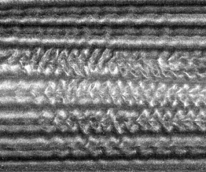
In order to examine the nature of the wavy instability in more detail, the frequency maps can be examined over a relatively short number of cycles, such that the change in the Reynolds number is relatively small. Such ‘snapshots’ of the flow map over 20 cylinder revolutions are shown in figure 12 for four polymer solutions at  $Re = 700$. The changes in
  $Re$ over the course of each snapshot are less than 6.5. The wavy instability can clearly be seen in figure 12(a) (the Newtonian case), with several dark ridges undergoing periodic oscillations. These dark ridges correspond to the inward and outward jets between vortices, where the flat surfaces of the mica flakes are facing perpendicular to the direction of light and the viewing angle of the camera, resulting in a lack of reflected light in the images. The amplitude of the waves tends to be highest near the centre of the flow cell (
 $z/d \approx 11$), as was noted by Crawford et al. (Reference Crawford, Park and Donnelly1985) for a large aspect ratio (
 $\varGamma = 70.4$).

Figure 12. Brief ‘snapshots’ of the flow maps at  $Re = 700$ for four suspensions of xanthan gum; 0 ppm
  $(a)$, 50 ppm
  $(b)$, 100 ppm
  $(c)$ and 500 ppm
  $(d)$.
It is interesting to note that even within a given region of the flow cell, the amplitude of the waves is not the same at all jets. In fact, the amplitude appears to alternate, with every second jet having a relatively large amplitude and every other jet having a relatively weak amplitude. The no slip condition at the ends means that the first jet near the ends (i.e. one vortex spacing away from the end walls) move fluid radially outward (Imomoh et al. Reference Imomoh, Dusting and Balabani2010; Cagney & Balabani Reference Cagney and Balabani2019b); using this information, it can be seen from figure 12(a) that the wavy instability is strongest at the inward jets and relatively weak at the outward jets, regardless of the axial location.
The tendency for the waves to occur predominantly at the inward jets can also be seen in the flow map for the dilute solution of 50 ppm (figure 12b). However, as the concentration is increased further, this trend breaks down and the amplitudes of the waves appear approximately equal regardless of the direction of the jets (figure 12c,d).
Snapshots captured at a range of Reynolds numbers for the most viscoelastic case ( $c = 2000\ \textrm {ppm}$) are shown in figure 13. In many cases, the jets do not appear to follow a simple sinusoidal motion, reflecting the presence of multiple frequency components, as was indicated by the frequency map shown previously (figure 8b). This is most evident in the fluctuations at
  $Re = 350$ in figure 13(b), where the corresponding point in the frequency map in figure 8(h) indicate that much of the energy occurs at
  $f/N = 0.25$, but other ridges can be seen in the frequency map in the range
  $0.25 < f/N < 1$.

Figure 13. Brief ‘snapshots’ of the flow maps at various Reynolds numbers for a solution of 2000 ppm xanthan gum.  $(a)$
$(a)$  $Re =250$.
  $(b)$
$(b)$  $Re =350$.
  $(c)$
$(c)$  $Re =500$.
  $(d)$
$(d)$  $Re =600$.
  $(e)$
$(e)$  $Re =800$.
  $(f)$
$(f)$  $Re =1000$.
As well as revealing the complexity of the wavy flow at a given time or Reynolds number, the snapshots in figure 13 also demonstrate that the instability varies significantly in both the axial direction and with  $Re$. Shortly after the onset of wavy flow, waves are visible throughout the flow cell (figure 13a), but the appearance and frequency of the instability has changed dramatically by
  $Re = 350$ (figure 13b), and by
  $Re = 500$ and 600 (figure 13c,d), the amplitude of many waves has been damped. While some periodicity is clearly present, it is not uniformly distributed, as reflected by the presence of a single, large amplitude wave appearing in near isolation at
  $z/d = 19.5$ in figure 13(c). The amplitude of the wavy instability has recovered by
  $Re = 800$ (figure 13e), with significant waviness at both inward and outward jets near the axial centre. Finally, at very high Reynolds number (
 $Re = 1000$ in figure 13f), several waves can be seen, which are made all the more apparent by the reduction in the number of vortices. However, in this case, the waves are only observed at the inward jets, as was observed for the Newtonian fluid.
The changes shown in figure 13 cannot be attributed to random fluctuations, as repeated experiments shown in figure 14 indicate that these complex transitions are largely repeatable. The relative complexity of the dense solution of xanthan gum is likely to be associated with the growing importance of elasticity. However, unlike the random ‘elastic turbulence’ seen in highly viscoelastic fluids (Groisman & Steinberg Reference Groisman and Steinberg2000), the transitions seen here for  $c = 2000\ \textrm {ppm}$ are in fact surprisingly predictable, illustrating the complexity of the dynamics of dense polymer suspensions at high
  $Re$.
$Re$.

Figure 14. Frequency maps found in four repeated experiments for the solution of 2000 ppm xanthan. The distribution of energy in each map is similar, indicating that the various transitions described here and in previous figures are not the result of random processes, but are a manifestation of the complex fluid dynamics of the system. The corresponding flow maps are shown in figure 17 and are discussed in § 3.4.  $(a)$ 2000 ppm, test 1.
  $(b)$ 2000 ppm, test 2.
  $(c)$ 2000 ppm, test 3.
  $(d)$ 2000 ppm, test 4.
3.3. Vortex merger and splitting
The axial wavelength of Taylor–Couette flow is characterised by the number of vortex pairs present, which is in most cases constant. However, it is clear from some of the results presented here that this is no longer the case when the concentration of polymers exceeds around 100 ppm and vortices appear to suddenly merge as  $Re$ is increased (figure 7). In order to characterise how the wavelength changes with Reynolds number for each of the solutions tested, the flow maps were first averaged into segments of
  $\Delta Re = 10$ to reduce the effect of noise or wavy flow, and the FFT was applied to each column of the averaged flow map to determine the dominant wavelength at that Reynolds number. The data points in the flow map within one diameter of either end were neglected, which meant that the FFT captured the effect of the gradual dilatation of the vortices near the centre of the flow cell as well as any sudden changes in wavelength. This meant that
  $\lambda (Re)$ is not constrained to be a rational number (
 $L$ divided by the number of vortex pairs), but instead can vary smoothly, as would occur for an infinitely long flow cell.
For the low concentration solutions (figure 15a), the wavelength shows relatively little variation with  $Re$, which is consistent with visual inspection of the flow maps in figure 7. The dilute polymer solutions (
 $c = 20\text {--}100\ \textrm {ppm}$) exhibit some fluctuations, reflecting a slight drift in the position of vortices that can be seen in figure 7(b–d), but the magnitude of the change is small. The wavelength of the dilute polymer solutions in figure 15(a) is larger than that in the Newtonian case, which can be attributed to the shear-thinning rheology of the working fluids in the present study, as noted in previous experimental and theoretical studies (Alibenyahia et al. Reference Alibenyahia, Lemaitre, Nouar and Ait-Messaoudene2012; Bahrani et al. Reference Bahrani, Nouar, Neveu and Becker2015; Cagney & Balabani Reference Cagney and Balabani2019b).

Figure 15. Variation in the wavelength of the flow maps as a function of Reynolds number for the eight fluids tested. The wavelength was determined using the peak of the FFT calculated from the flow map (averaged into bins of  $\Delta Re = 10$), as described in the text.
The variations in  $\lambda$ are much more complex when the xanthan gum concentrations are higher and the role of elasticity becomes important (figure 15b). For the 200 ppm case,
  $\lambda$ remains approximately constant for
  $Re < 600$, before undergoing a sharp increase at
  $Re \approx 660$ and another increase at around 800, which coincide with the merger events seen in figure 7(e). Likewise, the
  $\lambda$ signal for the 500 ppm solution is relatively constant until merger events cause variations at
  $Re \approx 550$ and 850. Gradual changes in
  $\lambda$ can also be observed slightly before and following these events.
For the strongly viscoelastic cases ( $c \geq 1000\ \textrm {ppm}$),
  $\lambda$ exhibits several sharp changes. Although the general trend is for the wavelength to increase with
  $Re$, the effect is not monotonic. This can be understood by referring to the corresponding flow maps in figure 7(g,h), where the various merger events cause vortices up to several
  $d$ away to adjust their size and position, contributing to the general unsteadiness in the
  $\lambda$ signals. Some gradual fluctuations in the wavelength can also be seen for
  $c \geq 1000\ \textrm {ppm}$, particularly in the range
  $Re = 150\text {--}400$, which are not associated with vortex merger events, and will be explored in more detail in § 3.4.
The sensitivity of the vortex merger events to hysteresis is examined in figure 16, which compares the flow maps for four solutions obtained when  $Re$ is increasing (a,c,e,g) and decreasing (b,d,f,h). The most notable difference between the accelerating and decelerating flow maps is the absence of any vortex mergers for
  $Re \gtrsim 200$ in the latter case. For the 200 ppm solution, as
  $Re$ is increased, two mergers take place, leading to an increase in wavelength, but as
  $Re$ is decreased the flow retains this larger wavelength until a vortex pair splits at
  $Re \approx Re_c$, reducing the wavelength of the flow briefly before it reverts to circular Couette flow. For the other three cases shown in figure 16(b–d) with larger concentrations of xanthan, the splitting process is more noticeable; as the cylinder is decelerated the flow again retains its large wavelength until close to
  $Re_c$, at which point several vortices split over a very narrow
  $Re$ range. Comparison of the flow maps in the left and right columns of figure 16 indicates that over the range
  $Re \approx 200\text {--}500$, more than one wavelength is stable. Such hysteresis in the number of vortices was also noted by Beavers & Joseph (Reference Beavers and Joseph1974) for a solution of PAA that was both shear-thinning and viscoelastic, and in the simulations of a (Newtonian) Oldroyd-B fluid by Lange & Eckhardt (Reference Lange and Eckhardt2001). The absence of such merger events in the literature on Taylor–Couette flow of inelastic, shear-thinning fluids cited in § 1, and its occurrence in the Newtonian fluid modelled by Lange & Eckhardt (Reference Lange and Eckhardt2001) implies that the process may be a consequence of the viscoelasticity rather than the shear-thinning.

Figure 16. Flow maps for four concentrations of xanthan; 20 ppm  $(a)$; 50 ppm
  $(b)$; 100 ppm
  $(c)$ and 200 ppm
  $(d)$. The flow maps in (a,c,e,g) were acquired as the cylinder was accelerated (and are the same data as presented in figure 7e–h), after which the Reynolds number was held constant for approximately five minutes, before the cylinder was decelerated using the same magnitude acceleration rate to acquire the data presented in (b,d,f,h). (a) 200 ppm – increasing
  $Re$. (b) 200 ppm – decreasing
  $Re$. (c) 500 ppm – increasing
  $Re$. (d) 500 ppm – decreasing
  $Re$. (e) 1000 ppm – increasing
  $Re$. (f) 1000 ppm – decreasing
  $Re$. (g) 2000 ppm – increasing
  $Re$. (h) 2000 ppm – decreasing
  $Re$.
$Re$.
In contrast to the transitions associated with the wavy instability, which appeared to be highly repeatable, the vortex merger events are not entirely repeatable, as can be seen in figure 17, which shows four repeated experiments performed using an identical protocol (i.e. the same fluid, temperature, acceleration rate and maximum rotation speed) for the 2000 ppm solution. There is a clear tendency for merger to occur at certain points, e.g. near the centre shortly after  $Re_c$ and near the top of the flow cell at
  $Re \approx 600$, but the sequence of merger events cannot be said to be repeatable. There are clear similarities between the merger locations in tests 3 and 4 (figure 17c,d), but the comparison with tests 1 and 2 (figure 17a,b) is less clear (although some similarities remain, such as the merger near the top of the flow cell at
  $Re \approx 550$).

Figure 17. Flow maps found in four repeated experiments for the solution of 2000 ppm xanthan. The white circles indicate the points where vortex merger occurs. The corresponding frequency maps are shown figure 14.  $(a)$ 2000 ppm, test 1.
  $(b)$ 2000 ppm, test 2.
  $(c)$ 2000 ppm, test 3.
  $(d)$ 2000 ppm, test 4.
The differences in the locations of merger events shown here make the similarity of the four corresponding frequency maps (figure 14) all the more striking, and suggest that the merger of vortices has relatively little influence on the frequency spectra of the overall flow.
The locations of the various vortex merger and splitting events observed from repeated experiments are summarised in figure 18, where the different symbols refer to the different tests runs performed (under identical conditions). There is a general tendency for the merger events from different runs to cluster in certain regions of the  $z/d - Re$ plane. This is particularly evident for the 500 ppm solution (figure 18b), but clusters can also be seen at
  $Re \approx 550$,
  $z/d \approx 16$ and
  $Re \approx 800$,
  $z/d \approx 2$ in figure 18(c) and at
  $Re \approx 600$ and 900,
  $z/d \approx 20$ in figure 18(d). A general tendency can be inferred from figure 18 for merger to occur near the top or bottom of the flow cell (as was suggested by Crawford et al. (Reference Crawford, Park and Donnelly1985) for Newtonian flows), especially for
  $c \geq 500\ \textrm {ppm}$. However, when the cylinder is decelerating, vortex splitting tends to be distributed along the axis.

Figure 18. Summary of the axial locations and Reynolds numbers at which merger or splitting of vortices was observed. All tests were performed under identical conditions, with the exceptions of the open symbols in which the Reynolds number was decreasing with time.  $(a)$ 200 ppm.
  $(b)$ 500 ppm.
  $(c)$ 1000 ppm.
  $(d)$ 2000 ppm.
Similar vortex merging processes have been observed at  $Re < Re_c$ in viscoelastic suspensions of polymers in which the instability is controlled by elasticity and the flow is dominated by isolated diwhirls (Groisman & Steinberg Reference Groisman and Steinberg1998). However, it is important to note that, neglecting the merger events which are sometimes observed shortly after the formation of the Taylor vortices (i.e. at
  $Re \approx Re_c$), the first vortex merger always occurs at
  $Re \approx 500$, regardless of the concentration or rheology (and despite the vast difference in
  $De/Re$). While the occurrence of merger or splitting is clearly linked to the rheology, the point at which these events take place appears to be independent of the magnitude of the elastic forces, suggesting that these events are controlled by shear-thinning rheology (as the shear rheology is incorporated into the definition of the Reynolds number) rather than viscoelastic effects.
Vortex merger in Newtonian Taylor–Couette flow has been associated with the wavy instability, which causes a progressive reduction in the width of vortices, until at a critical point a vortex becomes too thin and is subsumed as the vortices on either side merge (Park & Crawford Reference Park and Crawford1982; Ahlers, Cannell & Dominguez-Lerma Reference Ahlers, Cannell and Dominguez Lerma1983; Crawford et al. Reference Crawford, Park and Donnelly1985). However, in some cases, such as in the 500 ppm solution at  $Re \approx 560$ and in the viscoelastic regime (
 $c \geq 1000\ \textrm {ppm}$) near
  $Re_c$, vortex merger occurs in the absence of the wavy instability. In fact, when the flow is decelerating, vortex splitting is observed only in the TVF regime. Thus, it can be concluded that at least some of the jumps in wavelength seen in the polymer solutions cannot be attributed to the same mechanism as has been described for Newtonian fluids.
In order to investigate the physical mechanism responsible for vortex merger, we examine two cases involving merger occurring before and after the onset of wavy flow. Figure 19 shows details of the flow map of a merger event shortly after the formation of the Taylor vortices (before the onset of wavy flow) and one at a relatively high Reynolds number when the flow is unsteady.

Figure 19. Detail of the flow maps for two cases of vortex merger in a  $c = 2000\ \textrm {ppm}$ solution; before the onset of wavy flow
  $(a)$ and when the flow is unsteady
  $(b)$.
  $(a)$ 2000 ppm, test 5.
  $(b)$ 2000 ppm, test 2.
A noticeable difference between the two cases is that in the former, three bright bands merge to form a single line (figure 19a), while in figure 19(b), it is three dark bands that merge. This is a consequence of the different initial orientations of flakes prior to each merger event, i.e. mostly aligned parallel to the cylinder surface at onset of TVF at  $Re \approx 70$ in figure 19(a), and mostly aligned around fully developed Taylor vortices in figure 19(b).
The removal of a recently formed vortex pair shown in figure 19(a) appears to occur via a gradual reduction in size, starting at around  $Re = 70$, as the neighbouring vortices above and below widen, before the pair is completely diminished by
  $Re = 77$ and the wavelength has been increased. The flow map indicates that this process does not involve any spiralling motion as the neighbouring vortices of opposite sign become imbalanced and develop a net circulation as they merge, as occurs in quiescent fluid for two opposite-sign vortices of different magnitude circulation (Leweke, Le Dizés & Williamson Reference Leweke, Le Dizés and Williamson2016). Instead, it is likely to be the same process as reported in the axisymmetric (two-dimensional) simulations of Lange & Eckhardt (Reference Lange and Eckhardt2001) for
  $De/Re = 0.15$ and
  $Re \approx Re_c$.
In contrast to this gradual, smooth process, the merger event shown in figure 19(b) for  $Re > Re_{c,w}$ is highly unsteady. As the Reynolds number is increased from 695 to 710, the three jets (now represented by dark bands) gradually move closer together, possibly as a result of the general tendency noted earlier for most vortices near the centre of the flow cell to grow in size, resulting in the squeezing of other vortices. All three jets show some waviness, but even long before the merger event at
  $Re \approx 700$, the amplitude and frequency of the waves do not appear to be the same for each jet. As the jets move closer together, the amplitude of the wave at the centre jet increases dramatically at
  $Re \approx 705$, and by
  $Re \approx 712$ the amplitude is comparable to the width of the vortices above and below it. Finally, there is a sudden merger at
  $Re = 714$, and thereafter only a single jet is present. This new jet fluctuates with a large amplitude and at a significantly lower frequency than the wave at the centre jet prior to the merger near
  $Re = 705\text {--}714$, demonstrating that such merger events can have a significant effect on the nature of the wavy instability. These jumps in wavelength may be responsible for some of the many changes in the nature of the wavy instability along the cylinder axis that can be seen in the snapshots in figure 13.
It seems plausible that the merger events which take place for  $Re > Re_{c,w}$ are governed by the same mechanism envisaged by Park & Crawford (Reference Park and Crawford1982) (i.e. the amplitude of the waves growing large enough to subsume neighbouring vortices), but in this case the process also involves the shrinking of vortices due to a gradual drift, rather than occurring solely due to the effects of the wavy instability. This distinction may explain the relative unpredictability of the merger events in polymer solutions.
We can use the same approach to study the inverse process – the splitting and formation of new vortices as  $Re$ is decreased. Figure 20 shows a detailed section of the flow map for the
  $c = 1000\ \textrm {ppm}$ solution as
  $Re$ is decreased from 121 to 83 (note that the Reynolds number decreases from left to right). At
  $Re = 121$, the flow appears to be stable, with the exception of some local waviness at a vortex pair near
  $z/d = 16$, indicated by the label ‘A1’. By
  $Re \approx 112$, the amplitude of the local waviness has grown, and the flow map develops a cross-hatched pattern; this represents the spiralling of neighbouring vortices which was noted to be absent in the vortex merger described above. The vortices have ceased spiralling by
  $Re = 106$ and by
  $Re = 83$ two newly formed, stationary vortices are present (labelled ‘A2’ in figure 20).

Figure 20. Detail of the flow map for the 1000 ppm solution in which the Reynolds number is decreasing, showing the splitting and formation of new vortices. The entire flow map is presented in figure 16(h). Note that  $Re$ decreases from left to right.
The formation of the new vortex pair and the accompanying spiralling motion induces unsteadiness at points along the flow cell, and by  $Re = 106$ the vortex pair directly below (labelled ‘B1’) has also split and undergoes a spiralling motion for
  $Re \approx 105\text {--}90$, after which it has split to form four distinct vortices (labelled ‘B2’). The spiralling of the B1 vortices appears to trigger unsteadiness and splitting in the vortices at lower axial height (
 $z/d = 4{-}11$), suggesting that the splitting of a single vortex pair can induce a cascade of subsequent splitting events, which is responsible for the large number of new vortices formed in a narrow range of Reynolds numbers close to
  $Re_c$ seen in the right column of figure 18.
3.4. Wavelength drift
Throughout many of the flow maps in the weakly viscoelastic and viscoelastic regimes presented in this study, a very prominent feature is the gradual drift in the size and position of vortices. It can be seen from figure 16, which shows the effect of hysteresis for  $c \geq 200\ \textrm {ppm}$, that this drift appears to be linked to the vortex merger events, as merger events are triggered by gradual changes in the size of vortices (as discussed in the previous section), and inversely, vortices readjust their size and spacing in response to a sudden change in the mean wavelength following a merger event. However, drift is also observed in the absence of any merger or splitting events, such as in the range
  $Re = 200\text {--}400$ for
  $c \geq 1000\ \textrm {ppm}$ (figures 16g and 16h), and for
  $Re > 200$ for all cases in figure 16 when the Reynolds number is decreasing.
A similar phenomenon has been noted in Newtonian flows, which is induced by the wavy instability and involves the elongation of vortices near the centre of the flow cell and the compression of vortices near the ends in order to relieve the additional strain induced by the wavy motion (Park & Crawford Reference Park and Crawford1982). However, the absence of this process in the Newtonian flow map (figure 7a) and the increase in drift as the polymer concentration is increased suggests that drift is dependent not just on the wavy instability, but also on the shear-thinning and viscoelasticity of the fluid. As  $Re$ is increased, there is a general tendency for the central vortices to dilate, in agreement with previous studies (Park & Crawford Reference Park and Crawford1982), but as
  $Re$ is decreased, the flow maps in figure 16 do not indicate any general trends, with the direction of drift of individual vortices or jets changing in an apparently random manner.
In order to quantify the onset of drift, the flow maps were divided into segments with intervals of  $\Delta Re = 25$, each segment was averaged to form a single intensity profile, and each profile was cross-correlated with the profile from the preceding segment. The maximum of the cross-correlation coefficient,
  $R_{max}$, provides a quantitative measure of the uniformity of the flow map, with
  $R_{max} \approx 1$ for negligible drift and lower
  $R_{max}$ as drift becomes more prominent. By averaging the profiles over each segment, the information on the waviness is suppressed, allowing the cross-correlation coefficient to yield information on low frequency changes in the position and size of vortices rather than high frequency phenomena. However, as vortex merger appears to be inherently coupled to the drift process (and has a dramatic effect on the flow maps),
  $R_{max}$ will be strongly influenced by such sudden changes in wavelength.
The variation in the maximum cross-correlation coefficient with Reynolds number for the eight fluids is plotted in figure 21. For the Newtonian case and solutions with moderate concentrations of xanthan ( $c \leq 100\ \textrm {ppm}$),
  $R_{max}$ remains relatively constant and close to unity, with the exception of a small region near
  $Re_c$, which likely arises due to the effects of the transition from CCF to TVF. There is a slight reduction in the
  $R_{max}$ signals for
  $c = 50\ \textrm {ppm}$ and 100 ppm near
  $Re \gtrsim 750$, which is a reflection of the moderate levels of drift seen in the flow maps (figure 7c,d). In contrast, the cross-correlation coefficient signal for
  $c = 200\ \textrm {ppm}$ decreases dramatically at
  $Re = 625$, which coincides with a merger event and the onset of both the wavy instability and significant drift. The drift is particularly evident in figure 7(e) near the top and bottom of the flow map. The
  $R_{max}$ signals become strongly disorganised as the xanthan gum concentration is increased; for
  $c = 500\ \textrm {ppm}$, the signal exhibits three sudden drops in amplitude (only two of which coincide with merger events), while the signals for the strongly viscoelastic solutions (
 $c \geq 1000\ \textrm {ppm}$) are characterised by spikiness throughout the entire
  $Re$ range, reflecting the continuous drift seen in the flow maps (figure 7g,h).

Figure 21. Variation in the maximum cross-correlation coefficient calculated for successive segments of the flow maps (averaged into segments of  $\Delta Re = 25$) with Reynolds number. The magnitude of
  $R_{max}$ provides a measure of the consistency of the flow structure, with a decrease in
  $R_{max}$ indicating that drift is occurring.
Examination of the cross-correlation coefficients in figure 21 suggests that the Reynolds number at which drift is observed appears to be reduced as the polymer concentration and shear-thinning increase. In order to test this observation using all the flow maps acquired for increasing  $Re$, a criterion was developed by which the critical Reynolds number for the onset of drift,
  $Re_{drift}$, coincides with the first points above
  $Re = 200$ when
  $R_{max}$ drops below 0.9. The requirement that
  $Re > 200$ is chosen to avoid the region near
  $Re_c$ where
  $R_{max}$ is reduced due to the establishment of TVF and the corresponding readjustment of the mica flakes.
What variations are sufficient to be classified as drift is an inherently subjective choice, and the use of the critical value of 0.9 is somewhat arbitrary; nevertheless, the variations in  $Re_{drift}$ were found to be qualitatively very similar to those found using other values of
  $\Delta Re$ and critical
  $R_{max}$, and the resulting estimates of
  $Re_{drift}$ give a good intuitive measure of the effect of the polymer concentration and rheology on the drift process, as can be seen from the flow maps.
The variation in the estimates of  $Re_{drift}$ with polymer concentration,
  $\overline {n_e}$ and
  $De/Re$ is shown in figure 22. Using this criterion, no drift is detected for
  $c < 50\ \textrm {ppm}$, which is consistent with visual inspection of the flow maps in figure 7(a,b). Above this concentration, the onset of drift decreases significantly with
  $c$, both in the weakly viscoelastic and viscoelastic regimes.

Figure 22. Variation in the Reynolds number at which significant axial drift of vortices is observed as a function of polymer concentration  $(a)$, effective flow index
  $(b)$ and elasticity
  $(c)$. The onset of drift is determined from the cross-correlation signals in figure 21, as outlined in the text. Each data point corresponds to a single test run, as detailed in table 2.
The presence of drift in both regimes, and the fact that  $Re_{drift}$ declines both with decreasing
  $\overline {n_e}$ and increasing
  $De/Re$, indicate that the drift cannot be attributed to either rheological phenomenon alone. However, it is interesting to note the similarities between the drifting vortices in the high concentration solutions and the isolated diwhirls seen in Newtonian viscoelastic fluids (Boger fluids) at low
  $Re$ (Groisman & Steinberg Reference Groisman and Steinberg1997, Reference Groisman and Steinberg1998; Martinez-Arias & Peixinho Reference Martínez-Arias and Peixinho2017). Diwhirls are typically observed at random locations along the axis rather than having a uniform spacing (Martinez-Arias & Peixinho Reference Martínez-Arias and Peixinho2017), suggesting that elastic instabilities in a Taylor–Couette geometry can occur at any wavelength. The data presented in the various flow maps in this study indicates that vortices in polymer solutions may be characterised by more than one wavelength at a given time, even in the inertial regime (
 $Re > Re_c$) and when the rheology is dominated by shear-thinning rather than viscoelasticity (i.e. in the weakly viscoelastic regime).
4. Effect of acceleration rate
An additional test was performed in order to assess the possible effects of the non-quasi-static acceleration rate used in the experiments on the results presented in § 3, such as the absence of purely elastic instabilities, the regime path ( $\textrm {CCF} \to \textrm {TVF} \to \textrm {WVF}$) and the presence of phenomena such as drift and spontaneous vortex merger/splitting.
For the highest concentration case,  $c = 2000\ \textrm {ppm}$, the cylinder was accelerated extremely slowly,
  $\mathrm {d}\omega /\mathrm {d}t = 0.004\ \textrm {rad} \ \textrm {s}^{-1}$, up to a maximum speed of
  $110.6\ \textrm {rad} \ \textrm {s}^{-1}$, which corresponds to
  $Re = 735$. The experiment lasted over
  $7\ \textrm {h}$, and images were acquired in six batches at a frame rate of 24 Hz. This is below the Nyquist frequency at high
  $Re$, leading to some aliasing effects in the frequency maps.
These conditions corresponded to an acceleration rate of  $\mathrm {d}Re/\mathrm {d}t^* < 0.03$ (2.2) throughout the entire test, and the variation in
  $\mathrm {d}Re/\mathrm {d}t^*$ with Reynolds number is shown in figure 23, along with the acceleration rate used in the other
  $c = 2000\ \textrm {ppm}$ tests discussed previously. The very low non-dimensional acceleration rate (
 $\ll 1$) ensures that the test can be treated as quasi-static (Dutcher & Muller Reference Dutcher and Muller2009). This test was only possible in a very dense polymer suspension, because in less concentrated suspensions the relatively low viscosity would increase the duration of the experiment (which approximately scales with
  $\mu ^{-1}$) and increase the risk of sedimentation of the mica flakes used for visualisation (the settling velocity also scales with
  $\mu ^{-1}$). The combination of these effects meant that as the cylinder speed was slowly increased throughout the CCF regime, sedimentation lead to an increase in the concentration of particles near the bottom of the flow cell and a depletion near the top, which in turn can affect the onset of instabilities (Gillissen & Wilson Reference Gillissen and Wilson2018). Any effects of sedimentation, such as those that occur between experiments, could easily be reversed by running the system in the WVF regime for a short period of time to redisperse the mica flakes, but this was obviously not possible mid-experiment.

Figure 23. Variation in the non-dimensional acceleration rate (2.2) with Reynolds number for two experiments performed with a  $c = 2000\ \textrm {ppm}$ solution. The higher acceleration case (dashed grey line) has been discussed in the previous sections.
The compiled flow map and frequency map for the very slow experiment are presented in figures 24 and 25, respectively, along with the corresponding maps for  $c = 2000\ \textrm {ppm}$ discussed earlier (see figures 7h and 8h). The white patches in the compiled maps correspond to the gaps between the video recordings, while the data was saved from the camera. The gaps are not uniformly distributed because
  $Re$ does not increase linearly with time.

Figure 24. Flow maps for a  $c = 2000\ \textrm {ppm}$ solution, with in which the cylinder rotation speed is increased quasi-statically
  $(a)$ and at a faster rate
  $(b)$. The white stripes in
  $(a)$ correspond to the periods where no images were recorded as the data was loaded from the camera. The corresponding non-dimensional acceleration rates are shown in figure 23, and the data in
  $(b)$ has also previously been presented in figure 7.
  $(a)$
$(a)$  $(\textrm {d}Re/\textrm {d}t^*)_{mean}=0.0317$.
  $(b)$
$(b)$  $(\textrm {d}Re/\textrm {d}t^*)_{mean}=1.81$.

Figure 25. Frequency maps for a  $c = 2000\ \textrm {ppm}$ solution, with in which the cylinder rotation speed is increased quasi-statically
  $(a)$ and at a faster rate
  $(b)$. The white stripes in
  $(a)$ correspond to the periods where no images were recorded as the data was loaded from the camera. The corresponding non-dimensional acceleration rates are shown in figure 23, and the corresponding flow maps are shown in figure 24. The data in
  $(b)$ has also previously been presented in figure 7. The black and white dashed lines represent the rotation speed of the inner cylinder. The rotation speed increases linearly with time; however, aliasing effects in
  $(b)$ cause the rotation frequency to appear to decrease at high
  $Re$.
$Re$.  $(a)$
$(a)$  $(\textrm {d}Re/\textrm {d}t^*)_{mean}=0.0317$.
  $(b)$
$(b)$  $(\textrm {d}Re/\textrm {d}t^*)_{mean}=1.81$.
Figure 24 indicates that a number of vortex merger events take place for  $Re \geq 500$ in both cases, regardless of the acceleration rate. As with previous cases (figure 18d), these appear most likely to occur near the top or bottom of the flow cell. Considerable drift in the position of vortices can also be seen in figure 24(a). The compression of a very long experiment into a single map in figure 24(a) gives the impression that these changes in position for
  $Re \gtrsim 600$ are quite rapid or constitute wavy behaviour, whereas in fact they occur slowly over long time spans.
The frequency maps for both cases also show a number of similarities (figure 25). The spectra in figure 25(a) were compiled using more data points and have a higher resolution (with each FFT spectrum calculated using 513 images, and acquired at intervals of  $\Delta Re = 1$), leading to a ‘cleaner’ map with more sharply defined ridges. Aliasing effects also cause the cylinder rotation frequency (black and white dashed line) to appear to ‘bounce’ off the top of the graph. Aside from these incidental differences, the maps are remarkably similar, with both maps being dominated by a dark ridge starting at approximately
  $f/N_{max} \approx 0.15$ and
  $Re \approx 250$ and continuing until approximately 380, a second, slightly weaker ridge starting at
  $f/N_{max} \approx 1.5$ and
  $Re \approx 150$ and another ridge starting at
  $f/N_{max} \approx 0.3$ and
  $Re \approx 300$. There are some ridges that do not match, the most notable of which is a short ridge at
  $f/N_{max} \approx 0.05$ and
  $Re \approx 100\text {--}130$ in figure 25(a). This wavy behaviour can also be seen directly in the corresponding flow map (figure 24a). However, similar ridges can be seen in the corresponding flow maps in figures 14(c) and 14(d), performed under the same conditions as the ‘fast’ map in figure 24(b).
The most significant observation regarding figures 24 and 25 is the absence of any instabilities associated with elasticity (diwhirls, disordered oscillations etc.), despite the very high elasticity and the negligible acceleration rate. The work of Groisman & Steinberg (Reference Groisman and Steinberg1998) predicts that for a polymer solution of this elasticity, disordered oscillations should occur throughout almost the entire  $Re$ range examined (see a reproduction of their regime map in figure 9). The absence of such elastic regimes indicates that the suppression of elastic instabilities in the current experiments is not a consequence of any unsteady effects, providing further evidence that shear-thinning rheology plays a very significant role in controlling the stability and dynamics of Taylor–Couette flow of non-Newtonian fluids.
5. Conclusions
The effect of shear-thinning and viscoelasticity on fluid instabilities in Taylor–Couette flow has been studied using a range of solutions of xanthan gum in a glycerol–water mixture. The concentration was varied over a wide range,  $c = 0\text {--}2000\ \textrm {ppm}$, and rheological tests indicated that this spanned the inelastic (
 $De \ll 1$), weakly viscoelastic (
 $De/Re \ll 1$) and viscoelastic (
 $De/Re \gtrsim 0.1$) regimes. Flow visualisation was performed by dispersing a small quantity of anisotropic flakes in the fluid, which allowed the flow field to be characterised as the Reynolds number was slowly increased up to 1000. Despite the high polymer concentrations examined, the flow did not exhibit any of the characteristic features of viscoelastic fluids, such as standing waves, disordered oscillations or diwhirls, which have been observed in several previous studies of Boger fluids for similar ranges of
  $De/Re$. The suppression of these modes was attributed to the shear-thinning rheology.
The polymers were found to lower the critical Reynolds number for the onset of Taylor vortex flow, but in the inelastic and weakly viscoelastic regimes the transition to wavy flow was delayed as the concentration was increased. The frequency of the wavy instability was also reduced from  $f_w/N \approx 0.76$ to
  $\approx 0.48$ as the concentration was increased. This transition occurred in a piecewise manner at
  $Re \approx 900$ for
  $c = 100\ \textrm {ppm}$. In the Newtonian and very dilute fluids, the wavy instability tended to occur predominantly in the centre of the flow cell (away from the ends) and at the inward jets. However, as the concentration was increased, the wavy instability tended to occur with comparable amplitude at both inward and outward jets.
In the viscoelastic regime there were distinct changes in the nature of the unsteady flow, which no longer occurred at a single frequency relative to the cylinder rotation speed. The flow became unsteady shortly after the formation of the Taylor vortices, and as  $Re$ was increased, the wavy instability underwent a number of transitions. Fourier analysis of the flow visualisation measurements showed that the unsteady flow varied substantially as the Reynolds number increased, with a number of frequency components appearing and diminishing, either gradually or abruptly, as
  $Re$ was varied. Examination of repeated experiments performed under identical protocols indicated that this process of transitions was remarkably repeatable, highlighting the impact of viscoelasticity on the level of complexity of the system.
In both the weakly viscoelastic and viscoelastic regimes, vortices were observed to merge as the Reynolds number was increased, leading to sudden changes in wavelength. This process has been noted in previous studies of shear-thinning or viscoelastic fluids (Beavers & Joseph Reference Beavers and Joseph1974; Lange & Eckhardt Reference Lange and Eckhardt2001), but has not been studied in detail. Experiments in which the Reynolds number was slowly increased and then slowly decreased revealed that this process is strongly hysteretic, with spontaneous splitting of vortices (decrease in wavelength) occurring as  $Re$ was reduced close to
  $Re_c$. Splitting was found to occur in two different manners, depending on whether the flow was steady or unsteady. When the flow was steady (
 $Re < Re_{c,w}$), the vortices merged in a gradual fashion which appears to be axisymmetric and similar to that described in the numerical simulations by Lange & Eckhardt (Reference Lange and Eckhardt2001). In the case of unsteady flow, merger tended to occur as a result of the gradual reduction in the size of a single vortex pair until it became comparable in size to the amplitude of the waves at the local jets, leading to a sudden removal of the vortices, which occurred over a time span comparable to the period of the local wavy instability.
Splitting of vortices as the Reynolds number was slowly reduced also occurred in a highly unsteady manner, with the newly formed vortices spiralling around each other due to an imbalance in the angular momentum, as occurs in imbalanced vortex pairs in two-dimensional unconfined flows (Leweke et al. Reference Leweke, Le Dizés and Williamson2016). This unsteadiness was found to trigger splitting in other vortex pairs, leading to a cascade of splitting events over a relatively short range of  $Re$.
$Re$.
As the polymer concentration was increased and the fluid could no longer be considered inelastic, the vortices were found to experience a gradual drift in terms of size and axial position, which was closely linked to the vortex merger process. The drift generally involved a dilatation of vortices near the centre of the flow cell and a contraction of vortices near the ends, but unlike the variations in the waviness of the flow, this drift was not found to be repeatable. Increasing the polymer concentration tended to cause this drift process to begin at lower  $Re$ and its magnitude to increase.
Finally, data were presented from a very long experiment performed for the densest polymer solution ( $c = 2000\ \textrm {ppm}$), demonstrating that the key finding of this study, such as the suppression of elastic instabilities, vortex drift and the merger/splitting of vortices, cannot be attributed to transient effects or experimental conditions (i.e. the non-dimensional acceleration rate). The experiments reported here demonstrate the complexity of the dynamics seen in Taylor–Couette flow of polymer solutions, especially when the fluids exhibit both shear-thinning and viscoelasticity.
Acknowledgements
Financial support for this work from the Engineering and Physical Sciences Research Council (EPSRC) Manufacturing the Future programme (no. EP/N024915/1) is gratefully acknowledged. The authors would like to thank Dr A. Alvarez-Fernandez and Dr S. Guldin, Adaptive & Responsive Nanomaterials Group at University College London, for help with the molecular weight measurements, and Dr S. Peers for her advice on the polymer chemistry.
Declaration of interests
The authors report no conflict of interest.


