


1. Introduction
Shock-containing free jets frequently produce high-amplitude, discrete-frequency screech tones as the consequence of aeroacoustic resonance; a review of this phenomenon is provided in Edgington-Mitchell (Reference Edgington-Mitchell2019). Since Powell (Reference Powell1953a) first suggested that screech tones were produced through an interaction between shock waves and shear-layer vortical structures, the exact nature of the tone-generation mechanism has remained an open question. Broadly speaking, the existing theories can be separated into those assuming a distributed source (Powell Reference Powell1953b; Norum Reference Norum1983; Tam, Seiner & Yu Reference Tam, Seiner and Yu1986), and those assuming the screech tones are generated at a single location (Mercier, Castelain & Bailly Reference Mercier, Castelain and Bailly2017; Li et al. Reference Li, He, Zhang, Hao and Yao2019). Beyond the questions regarding source location, there are questions regarding the exact nature of the sound-producing interaction between the Kelvin–Helmholtz wavepacket and the shocks; extant models either propose the tones are generated by Mach wave radiation arising from an interaction between the instability waves and shock cells, (Tam, Parrish & Viswanathan Reference Tam, Parrish and Viswanathan2014), or via a shock/vortex interaction process termed shock leakage (Manning & Lele Reference Manning and Lele1998). The latter model is the focus of the present work.
Aeroacoustic resonance can generally be divided into four distinct processes: a downstream wave propagation, a downstream reflection, an upstream wave propagation and an upstream reflection. The downstream-propagating component in screech is widely accepted to be the Kelvin–Helmholtz wavepacket; the extraction of energy from the mean flow by such wavepackets is generally well predicted by stability theory (Cavalieri et al. Reference Cavalieri, Rodríguez, Jordan, Colonius and Gervais2013). It has recently been demonstrated that the growth of these wavepackets seems to be largely insensitive to the presence of shocks in the flow (Edgington-Mitchell et al. Reference Edgington-Mitchell, Duke, Wang, Harris, Schmidt, Jaunet, Jordan and Towne2019), at least for relatively weak shocks. The upstream-propagating wave was originally assumed to be a free-stream sound wave (Powell Reference Powell1953b), however, there is now evidence that it is instead an intrinsic mode of the jet itself. This intrinsic mode has been observed in subsonic free jets (Schmidt et al. Reference Schmidt, Towne, Colonius, Cavalieri, Jordan and Brès2017; Towne et al. Reference Towne, Cavalieri, Jordan, Colonius, Schmidt, Jaunet and Brès2017), impinging jets (Tam & Ahuja Reference Tam and Ahuja1990), grazing jets (Jordan et al. Reference Jordan, Jaunet, Towne, Cavalieri, Colonius, Schmidt and Agarwal2018), supersonic impinging jets (Gojon, Bogey & Marsden Reference Gojon, Bogey and Marsden2016; Bogey & Gojon Reference Bogey and Gojon2017) and, most recently, in screech (Edgington-Mitchell et al. Reference Edgington-Mitchell, Jaunet, Jordan, Towne, Soria and Honnery2018a; Gojon, Bogey & Mihaescu Reference Gojon, Bogey and Mihaescu2018; Mancinelli et al. Reference Mancinelli, Jaunet, Jordan and Towne2019). There is, however, evidence, at least for supersonic impinging jets, that the feedback loop can also be closed by free-stream sound waves (Weightman et al. Reference Weightman, Amili, Honnery, Soria and Edgington-Mitchell2017, Reference Weightman, Amili, Honnery, Edgington-Mitchell and Soria2019). The upstream-reflection mechanism is typically assumed to be governed by the receptivity of the near-nozzle shear layer to acoustic forcing, but the small time and length scales associated with the receptivity process make measurement extremely difficult; the majority of research in this area has been from a theoretical perspective (Barone & Lele Reference Barone and Lele2005; Beneddine, Mettot & Sipp Reference Beneddine, Mettot and Sipp2015; Karami et al. Reference Karami, Stegeman, Ooi, Theofilis and Soria2020). Theory predicts that the receptivity is a strong function of the nozzle lip geometry, and this is consistently borne out in experiment (Raman Reference Raman1997; Weightman et al. Reference Weightman, Amili, Honnery, Edgington-Mitchell and Soria2019). This paper will primarily be concerned with the process whereby the screech tones are generated, which is generally assumed to be the downstream-reflection mechanism.
While the majority of extant screech models, originating with Powell, assume that sound is generated at the shock tips, a mechanistic explanation for this phenomenon was only suggested relatively recently. The phenomenon of a vortex interacting with an essentially infinite plane shock is widely studied (Hollingsworth Reference Hollingsworth1955; Ribner Reference Ribner1959; Dosanjh & Weeks Reference Dosanjh and Weeks1965; Meadows, Kumar & Hussaini Reference Meadows, Kumar and Hussaini1991; Ellzey et al. Reference Ellzey, Henneke, Picone and Oran1995; Guichard, Vervisch & Domingo Reference Guichard, Vervisch and Domingo1995), but relatively little attention had theretofore been given to the interaction of a vortex with a shock reflecting off a free boundary. In the first in a series of papers from the Center for Turbulence Research (CTR) at Stanford, Manning & Lele (Reference Manning and Lele1998) presented a direct numerical simulation (DNS) of the interaction of a single oblique shock with instability waves in a finite thickness shear layer. During the passage of a vortex, a single cylindrical acoustic wave is generated at the tip of the shock. This shock tip also undergoes a deformation, following a circular path with the same rotational direction as the vortex, with the tip of the shock ‘leaking’ past the sonic line. The compression front associated with the acoustic wave is generated during the upstream motion of the shock, with a wavelength significantly shorter than the acoustic wavelength. To address some of the numerical issues with the scheme, a toy problem was constructed with the oblique shock replaced by a distribution of near-isentropic compression waves. The behaviour of the compression wave system was found to closely mimic that of the oblique shock, i.e. a section of the wave was observed to ‘leak’ and propagate to the far field. In both cases the emission of a wave from a single shock–vortex interaction was not observed to produce as strongly directional an acoustic field as observed in experiment.
This similarity between the near-isentropic approach and the full DNS motivated a series of ‘progressively idealized methods’ in Manning & Lele (Reference Manning and Lele2000). The first of these models was a linearized Euler approach. Here the (shock-free) shear layer was treated as the base flow, and the shock was implemented as a boundary condition; in combination with the resultant acoustic field this forms the perturbation field. Despite the significant simplification with respect to the original DNS, the linearized Euler equations produced the same apparent acoustic source mechanism as in the original full simulation, even showing strong quantitative agreement for the magnitude of the acoustic wave. A further simplification was the replacement of the shock with a Gaussian wave; the same mechanism of ‘leakage’ through the shear layer was observed. As an additional stage of model reduction, the base flow was replaced by a Stuart vortex mixing layer, and the mechanism was still preserved. This robustness was exploited to allow for the construction of a yet more idealized model based on geometrical acoustics. In this approach, the shock was replaced with a standing acoustic wave. The propagation of this wave is calculated through solution of the eikonal (ray-tracing) equation. The intrinsic value of this approach lies in its ability to quantitatively predict where and under what conditions the leakage phenomenon will occur. When vorticity in the shear layer is sufficiently strong, the wavefront normal is rotated back into the core of the flow, which the authors suggest is equivalent to a total internal reflection condition. Again using a Stuart vortex sheet model, the authors demonstrated that a perturbation of sufficient strength was needed to prevent the total internal reflection condition, and allow the wave to ‘leak’ past the sonic line. The theoretical framework for the shock-leakage model was further developed in work by Suzuki & Lele (Reference Suzuki and Lele2003), where both DNS and solutions to the eikonal equation were explored. Most critically, Suzuki and Lele determined that two parameters govern whether leakage occurs; the incident angle of the wavefront at the shear layer, and the strength of the vorticity at the point of reflection. The most recent theoretical development of the shock-leakage model is that of Shariff & Manning (Reference Shariff and Manning2013), where an extension to the geometrical acoustics approach is presented. This model forms the basis for much of the analysis in the present paper, and hence a detailed discussion is deferred to § 2.4.
The shock-leakage model for screech production is widely, but not universally, accepted. In addition to the work at the CTR, shock leakage has been qualitatively observed in large eddy simulations by Berland, Bogey & Bailly (Reference Berland, Bogey and Bailly2007). Experimental evidence for the phenomenon has remained somewhat limited, owing to the difficulty in measuring at the time and length scales required. An exception to the lack of experimental evidence is the ultra-high-speed schlieren visualizations performed by the authors, which have been presented in video form (Edgington-Mitchell, Honnery & Soria Reference Edgington-Mitchell, Honnery and Soria2014a; Edgington-Mitchell et al. Reference Edgington-Mitchell, Duke, Amili, Weightman, Honnery and Soria2015a, Reference Edgington-Mitchell, Weightman, Honnery and Soria2018b). Additionally, coherent vorticity measurements via particle image velocimetry (PIV) were used to argue for the shock leakage method in several screeching jet configurations (Edgington-Mitchell et al. Reference Edgington-Mitchell, Oberleithner, Honnery and Soria2014c; Edgington-Mitchell, Honnery & Soria Reference Edgington-Mitchell, Honnery and Soria2014b, Reference Edgington-Mitchell, Honnery and Soria2015b), however, only a qualitative argument was made. It should be noted that arguably shock leakage is visible in the remarkable video of Poldervaart, Vink & Wijnands (Reference Poldervaart, Vink and Wijnands1968), although the work of these authors predates the theoretical development of Manning & Lele (Reference Manning and Lele2000). One critique of the shock-leakage model is that sharp shock-like wavefronts should result from the process, which have not always been visible in flow visualization data. In planar and high-aspect rectangular jets, however, shock-like wavefronts have been consistently observed (Poldervaart et al. Reference Poldervaart, Vink and Wijnands1968; Raman Reference Raman1997). In the review of Raman (Reference Raman1998), it was suggested that these sharp wavefronts might arise from nonlinear steepening of the acoustic wavefront, however, the shock-leakage model suggests that the waves can be shock-like from their inception. In contrast, some past visualizations of jet screech from axisymmetric jets have presented a smoothly varying sinusoidal density gradient perturbation fields, such as those produced by Seiner (Reference Seiner1984), which at first glance seem inconsistent with the waves produced via shock leakage. Care must, however, be taken in the interpretation of such data for two reasons. Firstly, these oft-cited images are the result of a phase-averaging process, and any uncertainty or jitter in the phase angle will result in a smeared wavefront. Secondly, the path-integrated nature of schlieren can act to obscure the true nature of waves in non-planar fields.
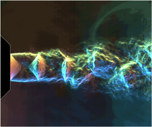
A flapping jet from an axisymmetric nozzle can produce sharp wavefronts similar to those observed in planar jets; an instantaneous colour schlieren image is presented in figure 1 for a jet screeching in the flapping B mode at a nozzle pressure ratio (NPR) of 2.6. A sharp acoustic wavefront is visible in the upper half of the image. Supposing that the acoustic wave propagates as either a cylindrical or spherical wave, a circle drawn through the wave can be used to determine the source origin; such a circle is overlaid on the image in the lower half of the figure, which has a phase offset of approximately  $180^{\circ }$. It can be observed that the acoustic wave appears to originate from the tip of the fourth shock cell at its point of greatest radial extension. Shock-like wavefronts in the acoustic near field are evidently not restricted to planar geometries, and in this paper it will be demonstrated that such waves can be observed for all oscillation modes in axisymmetric jets.

Figure 1. Instantaneous high-resolution colour schlieren image of jet at  $NPR=2.6$, screeching in the flapping ‘B’ mode. The white circle approximates the radius of the acoustic wave visible in the upper image.
The purpose of this paper is to rectify the deficit of experimental evidence for the shock-leakage phenomenon, and to further validate the extant linear models for the phenomenon. The evidence provided herein takes two forms: first, ultra-high-speed schlieren visualizations of the shock leakage phenomenon, and second, the application of the ray-tracing model of Shariff & Manning (Reference Shariff and Manning2013) to experimentally acquired velocity fields in screeching jets. Shock leakage is observed in toroidal and flapping modes of single jets, as well as in twin-jet systems. The paper is laid out as follows. In § 2 a discussion of the experimental methodology and data decomposition techniques is presented, along with a detailed recapitulation of the model of Shariff & Manning (Reference Shariff and Manning2013). Section 3 presents observations of shock leakage made via visualization techniques, while § 4 presents the quantitative predictions of the ray-tracing model. The paper concludes in § 5 with a discussion of where shock leakage occurs in the flow, and the factors that govern this localization.
2. Method and theory
2.1. Experimental database
All schlieren and some of the PIV experiments were conducted in the Laboratory for Turbulence Research in Aerospace and Combustion (LTRAC) Supersonic Jet Facility, with a subset of PIV experiments carried out in the newer LTRAC Gas Jet Facility. The two facilities are very similar in plenum construction, but the Gas Jet Facility has Perspex walls at a distance of  $60D$ (where D is nozzle exit diameter) from the nozzle centreline on all sides, changing the far-field boundary conditions. Both facilities are supplied with dry compressed air at a stagnation temperature of approximately 298 K, regulated to within
  $1\,\%$ of the target pressure by a Fairchild 100 high-flow pressure regulator. Pressure in the plenum chambers was monitored by an RS-461 pressure transducer with an uncertainty of
  ${\pm }0.25\,\%$. The same nozzle was used for all measurements: a 15 mm diameter purely converging nozzle, with a radius of curvature of 67.15 mm, ending with a 5 mm parallel section at the nozzle exit, and an external lip thickness of 5 mm. The plenum-to-nozzle contraction ratio is in excess of
  $100\,{:}\,1$. Given the short parallel nozzle section and high contraction ratio, the boundary layer at the nozzle exit is expected to be extremely thin and likely laminar. Both optical facilities contain numerous hard reflective surfaces, and thus can in no way be considered anechoic. Exemplar measurements of screech directivity were obtained in the LTRAC Supersonic Anechoic Jet Facility (SJAF), using a G.R.A.S. Type 46BE 1/4” pre-amplified microphone, recorded on a National Instruments DAQ at a sample rate of 250 kHz. The nozzle in this facility is smaller (
 $D=8\ \textrm {mm}$), with a lower contraction ratio; the boundary layer may be slightly thicker in this facility. The acoustic spectra presented in figure 2 both display the well-known directivity pattern of jet screech, which has been most carefully characterized in the work of Norum (Reference Norum1983). Norum identified that the fundamental screech tone radiated most strongly at
  $\phi =160^{\circ }$ (here
  $\phi$ is the polar angle measured from the downstream axis) across a wide range of pressure ratios and modes of jet screech. For the screech modes associated with azimuthal mode
  $m=1$, there was a minimum in screech tone amplitude at
  $\phi =90^{\circ }$, but a maximum for the first harmonic. In the present data, for the jet at
  $NPR=3.4$, the same trend is observed; increasing directivity of the fundamental as the observer is moved upstream, and a minimum in the sideline direction for the fundamental, but a maximum for the first harmonic. For the
  $NPR = 2.25$ jet, an increase in tone amplitude is observed as the observer is moved upstream, however, the effect is far less pronounced than for the higher-pressure ratio jet. The minimum for the fundamental at
  $\phi =90^{\circ }$ is also not observed for this condition. The present set-up of the SAJF cannot produce far-field data at the extreme upstream angles available in the data of Norum (Reference Norum1983), but the key trend of upstream directivity is evident even in the smaller range of angles available.

Figure 2. Representative far-field ( $50D$ from nozzle exit) acoustic spectra for various polar angles
  $\phi$, measured from the downstream axis. Symbols indicate peaks of the fundamental screech tone.
Several flow conditions are considered here in detail, covering several ‘stages’ of jet screech, as summarized in table 1. Flow visualizations are provided for some other cases beyond those listed in this table. Here, nozzle pressure ratio ( $NPR$) is defined as the ratio between the plenum and the ambient pressure:
  $NPR = p_0/p_{\infty }$, and ideally expanded Mach number
  $M_j$ is calculated assuming isentropic expansion to ambient pressure. Reynolds and Strouhal number are likewise calculated based on ideally expanded conditions:
  $Re=U_j \rho _j D_j / \mu$,
  $St=f_sU_j/D_j$. Here, U,
  $\rho$ and D refer to axial velocity, density and diameter respectively, with the subscript j indicating the ideally expanded condition. Note the slight correction of Strouhal numbers from those presented in Edgington-Mitchell et al. (Reference Edgington-Mitchell, Jaunet, Jordan, Towne, Soria and Honnery2018a).
Table 1. Jet conditions.

The schlieren images were obtained using various configurations of a classical Toepler Z-type schlieren apparatus with mirrors of focal length 2032 mm (Mitchell, Honnery & Soria Reference Mitchell, Honnery and Soria2012). High-speed schlieren images were acquired using a Shimadzu HPV-1 with a resolution of  $312 \times 260\ \textrm {px}$, using an exposure time of 250 ns. Illumination for the high-speed images was provided by a Metz Mecablitz flash. The schlieren imaging apparatus records an image whose intensity is proportional to the path-integrated density gradient, with a directionality determined by the orientation of the spatial cutoff. For the monochrome schlieren images, a standard razor blade is used as the spatial cutoff. The cutoff is oriented to capture the axial density gradient, such that the intensity of the images (
 $I$) in this paper represent
  $I(x,y) \propto \int \partial \rho /\partial x \, \textrm {d}z$; here
  $x$ is positive in the downstream axis,
  $y$ is the transverse direction and
  $z$ represents the path of integration orthogonal to the other two axes. High-resolution colour images were obtained by replacing the flash unit with a pulsed white LED (Willert, Mitchell & Soria Reference Willert, Mitchell and Soria2012) focused onto a four-colour mask. The knife edge was replaced with an iris cutoff, such that the direction of the density gradient is encoded in the colour of the resultant image.
The PIV datasets for the  $NPR = 2.10$ and
  $NPR = 2.25$ cases, which correspond to the toroidal ‘A’ mode of jet screech, were acquired in the LTRAC Gas Jet Facility and have previously been presented in Edgington-Mitchell et al. (Reference Edgington-Mitchell, Jaunet, Jordan, Towne, Soria and Honnery2018a). The dataset for the
  $NPR = 3.4$ case, which corresponds to a helical ‘C’ mode of screech, was obtained in the Supersonic Jet Facility, and has previously been presented in Edgington-Mitchell et al. (Reference Edgington-Mitchell, Oberleithner, Honnery and Soria2014c) and Tan et al. (Reference Tan, Soria, Honnery and Edgington-Mitchell2017). Pertinent details such as final interrogation window size
  $IW_1$, vector spacing
  $\Delta X$, through-plane integration distance based on light sheet or depth of field
  $Z$ and field of view
  $FOV$ are presented in table 2. For all cases the same seeding was used, in the form of 600 nm diameter smoke particles (Mitchell, Honnery & Soria Reference Mitchell, Honnery and Soria2013), and the multi-grid algorithm of Soria (Reference Soria1996) was used to analyse the image pairs. Contours of mean axial velocity for the three PIV datasets are presented in figure 3.

Figure 3. Mean axial velocity, normalized by jet exit velocity  $U_E$ for: (a)
  $NPR = 2.10$; (b)
  $NPR = 2.25$; (c)
  $NPR = 3.4$.
Table 2. PIV parameters.

2.2. Decomposition of velocity data
The PIV data presented here are not time resolved with respect to the screech frequency. Consequently the shock-leakage behaviour (which cannot be modelled as a steady process as per Shariff & Manning (Reference Shariff and Manning2013)) cannot be directly interrogated by analysing the raw data. However, reconstruction of a phase cycle of the screech phenomenon can facilitate assessment of shock leakage even if the original snapshots are statistically independent. Here, this phase reconstruction is done via a proper orthogonal decomposition (POD).
Although the flows considered in this paper are highly turbulent, the resonance process that produces the discrete-frequency screech tone is a result only of a series of coherent downstream-propagating wavepackets at one particular wavelength. Following Hussain & Reynolds (Reference Hussain and Reynolds1970), the fluctuations in the jet may thus be decomposed into a mean ( $\boldsymbol {U}$), coherent fluctuations at the screech frequency
  $\boldsymbol {u}^c$ and a stochastic component (
 $\boldsymbol {u}''$)
 \begin{equation} \boldsymbol{u}(\boldsymbol{x},t) = \boldsymbol{U}(\boldsymbol{x})+\boldsymbol{u}^{c}(\boldsymbol{x},t)+\boldsymbol{u}''(\boldsymbol{x},t). \end{equation}
 It has been demonstrated consistently in prior work that snapshot proper orthogonal decomposition (Sirovich Reference Sirovich1987) can extract the coherent component associated with the screech process. For the POD, the autocovariance matrix is constructed from the velocity snapshots  $\boldsymbol {V}$ such that
 \begin{equation} \boldsymbol{R}=\boldsymbol{V}^T\boldsymbol{V}. \end{equation}
The solution of the eigenvalue problem
 \begin{equation} R\boldsymbol{v}=\lambda \boldsymbol{v} \end{equation}
yields the eigenpairs ( $\lambda ,\boldsymbol {v}$) from which the spatial POD modes are constructed as
 \begin{equation} \boldsymbol{\phi}_n(x,y)=\frac{\boldsymbol{V}\boldsymbol{v}_n(t)}{\|\boldsymbol{Vv}_n(t)\|}. \end{equation}
The coefficients at each time  $t$ for each mode
  $n$ can be expressed as
 \begin{equation} \boldsymbol{a}_n(t)=\boldsymbol{v}_n(t)\|\boldsymbol{Vv}_n(t)\|. \end{equation}
Coherent fluctuations are reconstructed according to the sum of weighted modes
 \begin{equation} \boldsymbol{u}_c(\boldsymbol{x},t)=\sum^2_{n=1}\boldsymbol{\phi}_n(x)\boldsymbol{a}_n^T(t). \end{equation}
 If a pair of POD modes that represent a travelling wave can be identified, and if the coherent fluctuations can be represented only by a single pair of these modes, then the phase cycle associated with screech can be reconstructed directly from this POD modes pair (Oberleithner et al. Reference Oberleithner, Sieber, Nayeri, Paschereit, Petz, Hege, Noack and Wygnanski2011; Jaunet, Collin & Delville Reference Jaunet, Collin and Delville2016). By defining  $a_1 - \textrm {i}a_2=\hat {a}\textrm {e}^{-\textrm {i} \omega _s t}$, a phase angle can be associated with each snapshot.
The axial velocity fluctuations associated with the leading pair of POD modes for each case are provided in figure 4, along with a joint probability density function (JPDF) of the mode coefficients plotted against each other. The Lissajous curve overlaid on the JPDF in black represents the mean radius of the mode pair at each phase angle; the closed circle indicates that these pairs of modes represent a travelling wave structure (Taira et al. Reference Taira, Brunton, Dawson, Rowley, Colonius, McKeon, Schmidt, Gordeyev, Theofilis and Ukeiley2017). The radius here is analogous to the amplitude of the coherent fluctuations, and the distribution of the JPDF about the mean radius hence indicates a degree of variation in the strength of the coherent fluctuation. The effect of this fluctuation amplitude on the shock-leakage process is considered in § 5.

Figure 4. (a,d,g) Coherent axial velocity fluctuation association associated with first POD mode. (b,e,h) Coherent axial velocity fluctuation association associated with second POD mode. (c,f,i) Probability density of temporal coefficients for leading two POD modes. All contours are normalized by maximum value.
2.2.1. Decomposition of schlieren data
While the ultra-high-speed image sequences contain a wealth of information about the flow dynamics, the limitations of the experiment can make this information difficult to extract. Observation of shock leakage requires operating the camera at the limit of its capacity at one million frames per second. In this regime the signal to noise ratio is quite poor. The limitations of the schlieren technique are even more severe; in the jet near field the hydrodynamic fluctuations associated with downstream-travelling structures are significantly stronger than the fluctuations associated with the upstream-propagating acoustic waves produced by shock leakage. High sensitivity in the schlieren system is required to visualize the acoustic waves, but with a classical schlieren system there is an inverse relationship between measuring range and sensitivity; resolving the acoustic waves means the downstream-propagating structures saturate the schlieren image. In an attempt to educe only the components of the schlieren image associated with the shock-leakage phenomenon, a Fourier decomposition is performed on the data. Since shock leakage is the consequence of an upstream motion of the shock tip, and the conversion of a section of that shock tip into an upstream-propagating wave, the phenomenon is most clearly visualized only in components with negative (upstream) phase velocity. The intensity of the images is a function of both space and time:  $I(x,y,t)$, and can thus be decomposed as
 \begin{equation} I(x,y,t) = \sum_{k}\sum_{\omega}\hat{I}_{k,\omega}\textrm{e}^{\textrm{i}kx}\textrm{e}^{-\textrm{i}\omega t}. \end{equation}
 The data can then be filtered to show only components propagating upstream (i.e. axial wavenumber  $k < 0$) at the screech frequency
  $\omega _s$. The reconstructed intensity field can be written in terms of the temporal Fourier coefficient
  $\hat {a}$
 \begin{equation} I(x,y,t) = \hat{a}\textrm{e}^{-\textrm{i}\omega_s t}\sum_{k<0}\hat{I}_{k,\omega_s}\textrm{e}^{\textrm{i}kx}. \end{equation}
2.3. Coherent structure identification via fields of finite-time Lyapunov exponents
Shock leakage is expected to occur at the saddle point between vortices, where the local vorticity is a minimum (Suzuki & Lele Reference Suzuki and Lele2003). These saddle points and the shear layer can be identified in the velocity data through the use of Lagrangian coherent structures (LCS) (Haller Reference Haller2015). In addition to facilitating an objective definition of the saddle points, LCS also enable a more intuitive comparison between the structures observed in the flow visualizations of § 3 and the velocity data of § 4. In this work the identification of LCS is performed by tracking contours of maxima in the field of finite-time Lyapunov exponents (FTLEs), following the methodology of Premchand et al. (Reference Premchand, George, Raghunathan, Unni, Sujith and Nair2019).
The Lyapunov exponent measures the degree of attraction or repulsion between neighbouring packets of fluid. As the FTLE is tracked backwards in time, local maxima in the FTLE represent unstable manifolds in the flow; these unstable manifolds, defined as regions of where the fluid particles converge along material surfaces, are analogous to LCS in the flow field, which educes the shear layer. The Lyapunov exponent is defined as per
 \begin{equation} \sigma^T_{t_0}(\boldsymbol{x_0},t_0)=\frac{1}{|T|}\ln\sqrt{\lambda_{max}(C^t_{t_{0}}(\boldsymbol{x_0},t_0))}. \end{equation}
Here,  $C^t_{t_0}$ is the right Cauchy–Green tensor, defined from the Jacobian of a mapping of the flow field
  $F^t_{t_0} := x(t: t_0, \boldsymbol {x_0})$, as per (2.10). The gradient of the flow map
  $F$ is a
  $3\times 3$ matrix for a three-dimensional velocity field, termed the deformation gradient tensor. Its elements represent the gradient of the new location of a fluid parcel
  $\boldsymbol {x}$ with respect to its starting location
  $\boldsymbol {x_0}$, i.e.
  ${\partial \boldsymbol {x}}/{\partial \boldsymbol {x}_{\boldsymbol {0}}}$. The right Cauchy–Green tensor can be constructed by premultiplying the transpose of the deformation gradient tensor with itself and represents the square of the local changes in fluid displacement. This eliminates the effects of a pure rotation of the fluid parcel and provides a rotation-independent deformation metric.
 \begin{equation} C^t_{t_{0}}=\left[\boldsymbol{\nabla} F^t_{t_0}(\boldsymbol{x_0})\right]^\intercal \boldsymbol{\nabla} F^t_{t_0}(\boldsymbol{x_0}). \end{equation}
 As defined here,  $\sigma ^T_{t_0}(\boldsymbol {x_0},t_0)$ measures the separation rate of initially adjacent fluid particles over the time period
  $T=t_0-t={1.5}/{f_s}$.
Again, following the approach of Premchand et al. (Reference Premchand, George, Raghunathan, Unni, Sujith and Nair2019), in this work the particle advection is performed backwards in time, such that the maxima of the FTLE contours represent attracting rather than repelling LCS, as indicated in figure 5.

Figure 5. Schematic showing fluid parcel advection in forward time; the red line represents the forward time FTLE, and the blue line the backward time FTLE.
2.4. Geometrical acoustics model
Here, a summary of the fundamental precepts of the ray-tracing model of Shariff & Manning (Reference Shariff and Manning2013) is presented; for a full discussion the reader is referred to the original work. Following from the earlier work of Manning & Lele (Reference Manning and Lele2000), the shocks within the jet are treated as standing acoustic waves, whose behaviour is modelled using geometrical acoustics. In the implementation of Shariff and Manning, the waves are visualized as ‘streaks’ produced by continuously injecting particles that obey the ray-tracing equations. From the original ray-tracing equations in an unsteady base flow  $V_i$, where
  $x_i(t)$ is a position along a ray,
  $k_i(t)$ is the associated wave vector and
  $i$ is an index over the spatial dimensions
 \begin{equation} \frac{\textrm{d}x_i}{\textrm{d}t}=\frac{\partial \omega}{\partial k_i}, \quad \frac{\textrm{d}k_i}{\textrm{d}t}=-\frac{\partial \omega}{\partial x_i}. \end{equation}
Shariff and Manning demonstrate a reduction to the following form:
 \begin{gather} \frac{\textrm{d}x_i}{\textrm{d}t}= V_i + \frac{k_i c(\boldsymbol{x},t)}{|\boldsymbol{k}|}, \end{gather}
 \begin{gather} \frac{\textrm{d}k_i}{\textrm{d}t}= -k_j \frac{\partial V_j}{\partial x_i} - |\boldsymbol{k}| \frac{\partial c(\boldsymbol{x},t)}{\partial x_i}. \end{gather}
 Equation (2.12) dictates the that the change in particle position is determined by both advection by the base flow  $V_i$, and the wave's own propagation, with direction given by
  $k_i$ and velocity by
  $c$. Equation (2.13) links the change in wave propagation direction
  $k_i$ (refraction) to the mean flow velocity gradient
  ${\partial V_j}/{\partial x_i}$ and gradients in the local speed of sound
  ${\partial c(\boldsymbol {x},t)}/{\partial x_i}$. In the original theoretical conception of Shariff and Manning, the synthetic velocity field was time periodic. As has been shown in the preceding subsection, by construction the decomposed experimental data are also time periodic.
2.5. Shock-leakage model
The implementation of the geometric acoustics framework of Shariff & Manning (Reference Shariff and Manning2013) with the experimental data is accomplished via the following:
(i) The datasets described in § 2.1 are decomposed via the methodology presented in § 2.2. On the basis of this decomposition a screech cycle is reconstructed across 2000 representations of the reduced-order velocity field. Each ‘time step’ in this reconstruction represents a
 $0.18^{\circ }$ increment in one single phase cycle of the screech process.
(ii) The reconstructed coherent velocity fields are smoothed using a
$3\times 3$ Gaussian kernel.(iii) At each time step in the screech cycle, particles obeying the equations stated in § 2.4 are injected at the centreline of the first shock cell, with the wave angle
$\theta _k=\tan ^{-1}(k_2/k_1)$ set to the local Mach angle.(iv) All particles already injected into the flow evolve as per (2.12) and (2.13) at each time step.
(v) The process is repeated over 20 screech cycles.


In total, 40 000 particles are injected for each case. A few caveats must be placed on the interpretation of the results of this model. As no temperature data are directly available from the PIV measurements, the second term in (2.13) is neglected; the speed of sound is assumed to remain constant in the flow. The velocity fields reconstructed as per § 2.2 already contain shock structures, and these structures will influence the evolution of the particles in a way not intended in the original conception of the model. Attempts to model the temperature fluctuations from the PIV data were found to significantly exacerbate the effect of the shock structures in the base flow data; neglecting temperature fluctuation to some extent ameliorates the impact of these shocks. The model is only implemented in a two-dimensional sense, with planar base flow data. For the  $NPR = 3.4$ case, where the oscillations associated with the jet correspond to the
  $m=1$ mode, the model will not include the azimuthal velocity, which is significant. Even for the lower pressure ratio cases, the actual jet is axisymmetric, rather than planar. A cylindrical coordinate formulation would thus be more appropriate, but in the present work a planar model was used to enable direct comparison with the work of Shariff & Manning (Reference Shariff and Manning2013). Finally, note that in the original model there is a consideration given to wave energy and amplitude, but these properties are neglected in the present analysis. The model is sensitive to small variations in the experimental data, and to aid in interpretation, symmetry has been enforced about the jet centreline in the
  $NPR = 2.10$ and
  $NPR=2.25$ datasets by mirroring the data across the centreline. None of the results discussed in this paper are altered by this enforced symmetry, but there are fewer spurious ray streaks to complicate interpretation of the images. Given the numerous assumptions and simplifications in the implementation of the model, which is itself based on significant simplifications of the original physics, the strict predictive power of this implementation is obviously limited. However, with these caveats in mind, as shown in § 4, the model nonetheless performs remarkably well when compared to the flow visualizations presented in the following section.
3. Observations of shock leakage
As discussed in § 1, shock leakage is difficult to visualize directly. Not only does the phenomenon occur at very short time scales, but the density fluctuations associated with the acoustic waves are much smaller than those associated with the vortices and shocks. The path-integrated nature of schlieren means that the large hydrodynamic fluctuations often obscure the acoustic waves. Path integration adds further complications for both  $m=0$ and
  $m=1$ modes of jet screech; the former will produce a distributed axisymmetric source, the latter would produce a source constantly rotating around the shear layer of the jet (Umeda & Ishii Reference Umeda and Ishii2002). The image that results from an integration through the three-dimensional field associated with either of these source distributions is difficult to interpret. The easiest interpretation of flow visualization occurs when the jet is in a flapping mode; when viewed orthogonal to the direction of flapping the path integration introduces less ambiguity. In an axisymmetric jet, however, there is no preferred axis for the flapping mode. To obviate this difficulty, a twin-jet configuration will be considered first, where at certain operating conditions the flapping plane of the jets is fixed (Bell et al. Reference Bell, Soria, Honnery and Edgington-Mitchell2018; Knast et al. Reference Knast, Bell, Wong, Leb, Soria, Honnery and Edgington-Mitchell2018). Interpretation of this relatively straightforward case will then facilitate a discussion of a more canonical single axisymmetric jet.
3.1. Shock leakage associated with asymmetric screech modes
An image sequence for a twin-jet configuration with an internozzle spacing of  $s/D=3.0$ and
  $NPR = 3.1$ is presented in figure 6. The image has been cropped to only show a section of the lower jet. In figure 6(a), the fifth shock cell is indicated with a red arrow. In the raw image on the left of the panel, a large vortex associated with the Kelvin–Helmholtz wavepacket is visible just upstream of the shock. The processed image on the right of the panel retains only those components with an upstream phase velocity as per (2.8); the outer section of the shock is already tilting upstream as it interacts with the front of the vortex. As the vortex passes the shock in figure 6(b), the shock is observed to extend radially well past its quasi-steady-state position (although in a flow with such strong vortices, it is debatable whether a steady-state position truly exists). An acoustic wave produced by the upper jet is visible in this and subsequent figures, but is not yet relevant to the discussion. By figure 6(c) a section of the shock can be seen propagating away from the jet in a small arc, but within the jet the shock is no longer moving upstream. As the vortex moves downstream and away from the shock in subsequent panels, the sharp acoustic wavefront resulting from the shock leakage can be seen moving back upstream, highlighted with the red arrow in the final figure. As the leakage is occurring on the upper side of the jet, upstream tilting of the shock on the lower half of the jet in preparation for a leakage event on that side is already evident in figure 6(d) onwards. The video sequence from which figure 6 is extracted is presented in supplementary movie 1 available at https://doi.org/10.1017/jfm.2020.945.

Figure 6. Sequence of  $\textrm {d}\rho /{\textrm {d}x}$ schlieren images for a twin jet at
  $NPR = 3.1$, with
  $8\ \mathrm {\mu }\textrm {s}$ spacing between subsequent frames. On the left of each panel is the raw schlieren image. On the right of each panel is the result of the Fourier filtering to preserve only components with upstream phase velocity. The red arrows indicate the shock in (a), and the resultant acoustic wave in (f).
The same mechanism can be observed occurring at multiple points in both jets in a single image sequence, as demonstrated in figure 7. Here three discrete shock leakage events and their resultant acoustic waves are enumerated 1–3 as indicated in the figure. A series of videos demonstrating a range of shock-leakage examples for the twin-jet configuration are presented in supplementary movie 2.

Figure 7. Sequence of  $\textrm {d}\rho /{\textrm {d}x}$ schlieren images for a twin jet at
  $NPR = 3.1$. On the left of each panel is the raw schlieren image. On the right of each panel is the result of the Fourier filtering to preserve only components with upstream phase velocity. The arrows track three discrete shock-leakage events between frames. The panels span a period of
  $30\ \mathrm {\mu }\textrm {s}$ but are not equispaced in time; the interframe time is
  $20\ \mathrm {\mu }\textrm {s}$ and
  $10\ \mathrm {\mu }\textrm {s}$ respectively.
In single axisymmetric jets, it has long been recognized that the flapping ‘B’ screech mode is associated with the largest vortical structures and often the highest acoustic tone amplitudes. The precession of the flapping axis also makes the ‘B’ mode one of the most difficult to study, as both planar and path-integrated measurement techniques are sensitive to the orientation of the flapping axis. Figure 8 presents an image sequence capturing a flapping motion almost orthogonal to the viewing angle. In the image, the fourth shock cell (in the centre of the frame) is observed to produce a strong upstream-propagating wave via the same mechanism as observed for the twin-jet configuration. Supplementary movie 3 provides a range of examples of shock leakage in the flapping mode for a jet at  $NPR = 2.8$.

Figure 8. Sequence of  $\textrm {d}\rho /{\textrm {d}x}$ schlieren images for a single jet at
  $NPR = 2.8$ with
  $8\ \mathrm {\mu }\textrm {s}$ spacing between subsequent frames. On the left of each panel is the raw schlieren image. On the right of each panel is the result of the Fourier filtering to preserve only components with upstream phase velocity.
3.2. Shock leakage associated with axisymmetric screech modes
Figure 9 presents a series of visualizations of shock leakage occurring at the fourth shock cell for a jet at  $NPR = 2.25$, which is screeching in the ‘A2’ (
 $m=0$) screech mode. The phenomenon is significantly more difficult to observe here, so a schematic representation has been included in the figure to aid in interpretation. The process is consistent with the shock leakage model, and qualitatively similar to the mechanism observed in the flapping jets. Figure 9(a) shows a large toroidal vortex ring just upstream of the fourth shock cell. The Fourier-filtered image shows that the outer sections of the shock are already beginning to tilt upstream at this point. As the vortex passes the shock, the radial extension of the shock tip, followed by the emission of an upstream-propagating wave, are visible. Although the vortex is axisymmetric, as is the initial motion of the shock, in this particular image sequence the acoustic wave at the bottom of the jet is much more difficult to observe. This is emblematic of the difficulty in visualizing shock leakage in the
  $m=0$ mode. While at the point of generation the upstream-propagating wave is visible as a discrete wavefront, this wavefront will be generated around the entire azimuth of the jet. The schlieren image results from an integration of three-dimensional field generated by this distribution of waves, which means the initial sharp wavefront is rapidly smeared into one difficult to distinguish in a still image. The video sequence from which figure 9 is extracted is presented in supplementary movie 4.

Figure 9. Sequence of  $\textrm {d}\rho /{\textrm {d}x}$ schlieren images for a single jet at
  $NPR = 2.25$ with
  $8\ \mathrm {\mu }\textrm {s}$ spacing between subsequent frames. On the left of each panel is the raw schlieren image. In the centre of each panel is the result of the Fourier filtering to preserve only components with upstream phase velocity, with the dashed red rectangle indicating the zoomed region on the right of each panel; on the right is a schematic illustrating the shape of the upstream wave.
Figure 9 was selected as it provided a reasonably clear visualization of shock leakage in the  $m=0$ mode, but only at one shock tip. Figure 10 instead presents a sequence where shock leakage is visible at both the third and fourth shock cells, and on both the upper and lower sides of the jet. The resultant acoustic waves in this case are, however, far less clear. In figure 10(a), a vortex is visible having already passed the fourth shock cell. A weak shock-leakage event is highlighted at the fourth shock cell in the red circles. At the same time, a subsequent vortex is approaching the third shock cell, and in the Fourier-filtered image it can be observed that the upstream tilting of the outer portions of the third shock has commenced. In the subsequent images, even as shock leakage is occurring at the third shock cell (highlighted in figure 10e), the same vortex is beginning to induce the shock motion that is a precursor to shock leakage in the fourth shock cell.

Figure 10. Sequence of  $\textrm {d}\rho /{\textrm {d}x}$ schlieren images for a single jet at
  $NPR = 2.25$ with
  $8\ \mathrm {\mu }\textrm {s}$ spacing between subsequent frames. On the left of each panel is the raw schlieren image. On the right of each panel is the result of the Fourier filtering to preserve only components with upstream phase velocity. Red circles highlight shock-leakage events.
From consideration of the cases presented here, and of the much larger dataset omitted for brevity, some general statements can be made. Firstly, during interaction with a toroidal vortex, the entire shock moves upstream at the beginning of the shock-leakage process, with the degree of motion increasing with radius. This is consistent with the observations of Panda (Reference Panda1998) and André, Castelain & Bailly (Reference André, Castelain and Bailly2012). During interaction with a vortex associated with a flapping mode, the first few shock cells could be said to undergo both a radial translation and rotation. At the later shock cells, it is debatable whether it is accurate to discuss the shock as some kind of steady-state object that undergoes periodic perturbation. Instead, as previously demonstrated in Panda (Reference Panda1998) and also evident here, in the presence of the very large vortices associated with a ‘B’ type flapping instability, the conical oblique shock that is typically assumed does not really exist in an instantaneous sense: shocks form, split, translate and dissipate during the passage of the shear-layer vortices. During the passage of a vortex, the shock forms, then translates radially outwards. The outer part of the shock rotates in the upstream direction, before a section of it propagates away from the jet entirely. In both cases, a small section of the shock tip separates from the rest of the wave and begins to propagate, spreading out cylindrically (at least in a path-integrated representation). This is consistent with the ‘shock leakage’ as first described in Manning & Lele (Reference Manning and Lele2000); interaction with the vortex leaves the shock tip beyond the sonic line, and once the vortex moves downstream, this section of the shock must become upstream propagating to satisfy the governing equations. As it propagates, it expands radially and consequently begins to decay.
The shock-leakage process is stochastic and intermittent. In the case of the flapping single jet, the degree of intermittency is difficult to assess, due to the precession of the flapping plane. However, in the  $m=0$ single jet, leakage is sometimes visible from the third shock cell, sometimes the fourth, sometimes the fifth and sometimes all three. It is sometimes stronger on one side of the jet than the other. The extent of this variation is evident in supplementary movie 5, which presents a selection of recordings a jet at
  $NPR = 2.25$. In the twin-jet configuration the process is more regular, with leakage consistently observed at each of the shock cells visible in frame; however, large variations in the apparent strength of the resultant wave are evident in almost every image sequence. It must be emphasized that an absence of evidence is not necessarily evidence of absence; the limitations of the flow visualization technique mean that leakage may not always be observed even if it does occur. Nonetheless, it seems evident that there is variance in both the strength of the shock-leakage events and the size and strength of the shear-layer vortices. An explanation for this variation will be provided as part of § 5.
4. Predictions of shock leakage
The visualizations presented in the preceding section have indicated that shock leakage occurs in several different modes of jet screech, and at a range of source locations. In this section, the geometrical acoustics model is tested with real data, and used to determine the sensitivity of the position at which leakage occurs to variations in vortex strength. Given the limitations of the present model, particularly when combined with this dataset, it is worth considering how well the particle ray streaks match the actual shocks present in the flow. Figure 11 presents two axial velocity fields for the  $NPR = 3.4$ jet,
  $180^{\circ }$ out of phase, overlaid with particles as per § 2.5. In this figure, a filter has been applied to remove any particles without a sufficient number of neighbours, to isolate the strong wave generation at the third shock cell for clarity. For this operating condition the rays closely match the shock reflection points at the sonic line for the first three shock cells; by the fourth cell the agreement is still quite good but the particle tracks are less coherent. In each field presented in figure 11, the location of a shock-leakage event is highlighted with a red arrow, while the upstream-propagating wave resulting from the equivalent event on the opposite side of the jet is highlighted with a blue arrow. Upstream-travelling waves from further downstream are visible, the strongest of which correspond to the reflection of a particle track that represents an expansion fan rather than a shock wave. In supplemental movie 3 leakage from the fourth shock reflection point is also visible, however, very few particles are left at this point and the wave is far less clear. The agreement in shock reflection location between the underlying data and the model is excellent at
  $NPR = 3.4$, but somewhat poorer for the
  $NPR = 2.10$ and
  $NPR = 2.25$ cases, as indicated in figure 12. At these weakly underexpanded conditions, a significant fraction of the compression occurs through near-isentropic compression waves rather than discrete shocks, which may explain the poorer match between the data and the model. Nonetheless, the point at which leakage occurs may still be readily matched to the shock cells in the velocity field; leakage is first observed at the third shock cell for
  $NPR = 2.10$ (
 $x/D \approx 1.8)$, and at the fourth shock cell for
  $NPR = 2.25$ (
 $x/D \approx 3.0$).

Figure 11. Shock leakage predicted by the model at third shock cell for  $NPR = 3.40$. Red arrows indicate shocks at point of leakage, blue dashed arrows indicate waves arising from these events.

Figure 12. Comparison of leakage position. (a)  $NPR = 2.10$; (b)
  $NPR = 2.25$.
Figure 13 presents a view of the waves generated by the shock leakage model over a domain including a region upstream of the nozzle exit; note that there are no velocity data available for  $x/D \leq 0$ or
  $|y|/D \geq 1.5$ (the velocity is assumed to be zero where no data are available), and the model is of course unaware of the nozzle and flange upstream of the nozzle exit. While there are certainly differences between the two cases, there are also identifiable common features between them. Both generate waves that travel predominantly in the upstream direction, particularly from the first leakage site. Both also generate upstream-propagating waves from multiple sources, with variation in the apparent directivity of the waves from each source. In Powell's original conception of screech, the waves from sources further downstream should synchronize with those generated at upstream locations. It has since been pointed out by Tam et al. (Reference Tam, Seiner and Yu1986), and later acknowledged by Powell, Umeda & Ishii (Reference Powell, Umeda and Ishii1992), that this is not necessarily a requirement for screech. Nonetheless, the success of the original theoretical model of Powell (Reference Powell1953b) at predicting screech tones at some operating conditions indicates that this synchronization may indeed sometimes be a factor in frequency selection, since the model assumes wave superposition at the nozzle. In some of the schlieren visualizations, clear synchronization can be observed, and it was expected that the geometrical acoustics model, when applied to experimental data, might provide verification of this. Regrettably, since the spacing of the shocks in the model does not exactly match those in the experimental flow, it is difficult to draw any strong conclusions on this point. Thus while there is evidence for wave generation at multiple shock cells in both the schlieren data and the shock-leakage model, the role of wave synchronization in the upstream direction remains unclear. The spacing between waves from the same source matches the acoustic wavelength derived from the screech frequency, although this only serves as a validation for the model, given that the screech frequency was used to reconstruct the velocity fields associated with the screech cycle.

Figure 13. Far-field sound predicted by model. (a)  $NPR = 2.10$; (b)
  $NPR = 2.25$. Magenta lines indicate the
  $\phi = 160^\circ$ peak directivity predicted by Norum (Reference Norum1983).
Amongst the motivations for the multiple-source model of Powell (Reference Powell1953b) was a desire to explain the directivity pattern in jet screech; with an assumption of isotropic sources, the directivity could only be explained by the phased superposition of multiple sources. This directivity was explored in detail by Norum (Reference Norum1983), who showed that a phased array model matched data across a wide range of operating conditions for not only the fundamental, but the first three harmonics. However, the DNS of Manning & Lele (Reference Manning and Lele2000) and Suzuki & Lele (Reference Suzuki and Lele2003) suggests that the source is not necessarily isotropic. The first implementation of the geometrical acoustics shock-leakage model by Shariff & Manning (Reference Shariff and Manning2013) produced strong upstream directivity even without the need for superposition of multiple sources (though such superposition was also observed). In the present implementation of the model, strong directivity from individual sources is once again observed in the shape of the waves, although wave amplitude is not calculated. The present results do not conclusively prove directivity is driven at the source; the model used is linear, and the shocks are treated as infinitesimal perturbations. A qualitative comparison to the results of Norum (Reference Norum1983) is still possible, however; overlaid on figure 13 are magenta lines indicating an angle of  $phi = 160^{\circ }$ from the strongest source of leakage. For both cases, these lines bisect the strong upstream-propagating waves; these waves represent the largest coherent grouping of particles that have escaped from the jet. In the simulations of Shariff & Manning (Reference Shariff and Manning2013), these upstream-propagating waves also had the highest amplitude. Thus, while the limitations of the present model implementation must be kept in mind, the remarkable match between the wavefront normal and the measurement of Norum (Reference Norum1983) suggests that the peak directivity may well arise from a single source. As a further qualitative validation, the general shape of the waves produced by the model is very reminiscent of those observed in the schlieren of figure 6. The schlieren results must also be interpreted with care; the monochromatic schlieren is only capable of measuring gradients in the axial direction, and will thus accentuate components of waves travelling directly downstream or upstream. Nonetheless, while the relative strength of the upstream and sideline components can thus not be estimated from the schlieren, the system is equally sensitive in the upstream and downstream directions, and in the raw images there is little evidence of waves propagating downstream. Taken together, the flow visualization and geometric acoustics produce strikingly similar wave shapes, with both suggesting that the source itself is not isotropic, which further implies that superposition from multiple sources is not necessary to produce the observed far-field directivity. However, both visualization and model also demonstrate that there are multiple sources for sound emission, meaning that superposition may well remain a component of the directivity pattern. There are no significant qualitative differences in the model predictions between the
  $m=0$ and
  $m=1$ screech modes that would explain the significant variation in directivity observed in figure 2, however, the planar nature of the model limits what conclusions can be drawn from this lack of difference.
4.1. Shock-leakage processes
A time series demonstrating the leakage process is shown for  $NPR = 2.25$ in figure 14, with particles from the shock-leakage model in white, overlaid on contours of the Lyapunov exponent. As noted in figure 12, the furthest upstream position at which leakage occurs is at approximately
  $x/D \approx 3$. In the top image of figure 14, two particle streaks are intercepting the shear layer at this point; these correspond to the oblique shocks of the fourth shock cell. At this time in the phase cycle, these streaks are encountering the saddle point between vortices of the Kelvin–Helmholtz wavepacket, where strong reductions in local vorticity occur. Between the first and second images in figure 14, this reduction in vorticity allows the streak to leak out past the shear layer, and form a wavefront at approximately
  $x/D \approx 3$. This wavefront is strongly reminiscent of that observed in the schlieren sequences of figure 9(c). One-third of a screech cycle later, the wave can be observed propagating in the upstream direction, at
  $x/D \approx 2.5$.

Figure 14. Three points in the screech phase cycle, separated by  $120^{\circ }$, for a jet at
  $NPR = 2.25$. Colours represent magnitude of the Lyapunov exponent
  $\sigma$.
A similar series is presented for the  $NPR = 2.10$ jet in figure 15. At this condition, the fluctuations in vorticity are significantly stronger than for
  $NPR = 2.25$, as will be discussed in § 5. As a consequence of this increase in vorticity fluctuation, shock leakage occurs closer to the nozzle, with the first image showing the initiation of a leakage process at
  $x/D \approx 1.9$. By the second image, the wavefront generated by this leakage is visible extending well outside the jet shear layer, and by the third image it is propagating back to the nozzle at
  $x/D \approx 1.4$. Leakage from cells further downstream is again visible in these images. An animation of both cases, showing both the results of the ray-tracing model and the contours of FTLE maxima, is presented in supplementary movie 6.

Figure 15. Three points in the screech phase cycle, separated by  $120^{\circ }$, for a jet at
  $NPR = 2.10$. Colours represent magnitude of the Lyapunov exponent
  $\sigma$.
Figure 16 presents a magnified look at the fourth shock cell for  $NPR = 2.25$ during a shock-leakage process. Here, the Lyapunov exponent is represented by the black contour lines, the colour contours represent coherent vorticity fluctuations and the white dots are the particles from the shock-leakage model. The behaviour described in Suzuki & Lele (Reference Suzuki and Lele2003) and Shariff & Manning (Reference Shariff and Manning2013) is evident here: when a ray streak interacts with a vortex, it is reflected back into the core of the jet. When a streak instead interacts with a saddle point between vortices, a portion may leak past the sonic line if the fluctuation in vorticity is sufficiently strong, whereupon the streak then propagates upstream. To illustrate this, two exemplar particles are tracked in time in figure 16. The green diamond tracks a particle that reaches the centre of the shear layer of the jet coinciding with the arrival of a vortex, and the red circle tracks one that reaches the centre of the shear layer at a saddle point between vortices. The strong vorticity associated with the Kelvin–Helmholtz wavepacket acts to rotate the propagation direction of the green particle, reflecting it from the shear layer and redirecting it back towards the core of the jet. By contrast, the local minima in vorticity encountered by the red particle is insufficient to achieve a total internal reflection, and the particle is instead able to leak past the sonic line and propagate upstream.

Figure 16. Demonstration that ray streaks are reflected from vortices, but leak through saddle points, at the fourth shock cell for an  $NPR = 2.25$ jet. Black contours represent Lyapunov exponent
  $\sigma$, colour contours represent coherent out-of-plane vorticity. Green diamond and red circle each track a given particle across the three snapshots.
From the motion of the green particle in figure 16, it is evident that the interaction of the shock with the vortex drives the upstream translation of the shock, which acts as a precursor to the emission of the acoustic wave. It is, however, not until the shock encounters the saddle point between vortices that the leakage event occurs. This description appears consistent with the visualizations in figures 8 and 9; the upstream motion of the shock, as demonstrated in the Fourier-filtered images, begins with the arrival of the vortex. The emission of the upstream-propagating wave, however, does not occur until the vortex is well past the shock location; the results of the ray-tracing model provide an explanation for the observations in the high-speed schlieren.
5. Factors governing the location at which shock leakage occurs
Figures 11 and 12 suggest that the first leakage event occurs at different shock cells for different operating conditions; the third shock cell is the most upstream source for  $NPR = 2.10$ and
  $NPR = 3.40$, while it is the fourth shock cell for
  $NPR = 2.25$. From the work of Suzuki & Lele (Reference Suzuki and Lele2003) it was established that it is both the incident angle of the shock and the strength of the local vorticity fluctuation that determine whether or not a shock will leak. Shariff & Manning (Reference Shariff and Manning2013) demonstrated that, while a sufficiently strong vortex might result in a shock leaking at its first reflection point, for vortex trains of moderate strength multiple reflections are needed before a ray streak can leak beyond the jet boundary. Historically, it was generally accepted that screech tones would be produced when the shear-layer structures had grown sufficiently strong to interact with the shocks (Tam Reference Tam1995). In Edgington-Mitchell et al. (Reference Edgington-Mitchell, Oberleithner, Honnery and Soria2014c) the authors argued that instead of the overall amplitude of the fluctuations, it was the degree of variation in vorticity at the high-speed side of the shear layer that was the determining factor, i.e. leakage would likely occur where coherent vorticity fluctuations were a maximum. The present implementation of the shock-leakage model for a number of cases permits a reconsideration of this argument. Figure 17 presents contours of the magnitude of coherent vorticity fluctuation for the three cases presented in § 4. It is apparent that the magnitude of vorticity fluctuation is significantly lower for the
  $NPR=2.25$ case, where leakage does not occur until the fourth shock cell, than in either of the other two cases, where leakage is predicted at the third cell. Perhaps the more significant result, however, is that the leakage does not occur for
  $NPR = 2.25$ until well downstream of the point of maximum vorticity fluctuation. At
  $NPR = 3.40$ the most upstream leakage point is associated with a point of maximum vorticity fluctuation; at
  $NPR = 2.10$ the peak vorticity is slightly lower but the radial integral of vorticity is close to a maximum at the point where leakage occurs. At
  $NPR = 2.25$, however, the magnitude of the vorticity fluctuation has decreased significantly from its maximum value by the point at which leakage occurs. At this condition the weakening of vorticity at the saddle points coincident with the third shock reflection is insufficient to permit leakage. It is, however, evidently strong enough to alter the incident ray angle at the fourth shock reflection point such that leakage can occur, despite the axial decay of vorticity fluctuation magnitude.

Figure 17. Magnitude of coherent vorticity fluctuations, overlaid with point closest to nozzle where shock leakage is first observed. Green diamond indicates downstream limit of shock prior to commencement of leakage. (a)  $NPR = 2.10$; (b)
  $NPR = 2.25$; (c)
  $NPR = 3.40$.
The model suggests that shock leakage will occur from multiple axial locations. Indeed, the model likely underpredicts the extent to which this occurs, as the particle streaks have become quite difficult to distinguish after many reflections. The contours of figure 17 demonstrate that the vorticity fluctuations decay relatively slowly relative to the spacing of the shocks. Given this slow decay and the fact that the shocks remain significant for many nozzle diameters downstream of the first leakage point, inevitably there must be multiple axial stations at which shock leakage will occur. The flow visualizations in § 3 support this conclusion, providing examples of leakage occurring at multiple shock cells in figures 7 and 10.
While the model predicts variation between the most upstream leakage location for different jet operating conditions, as noted at the end of § 3, significant variations are observed even at fixed operating conditions; shock leakage is sometimes observed as beginning at the third shock cell for  $NPR = 2.25$, but at other times cannot be observed until the fifth shock cell. The experimental data and the geometrical acoustics model provide an explanation for this observed variation. The temporal coefficients for the POD modes representing screech, presented in figure 4, are scattered around the line of mean radius with an approximately normal distribution. This is indicative of variation in the strength of the vortical structures between snapshots (Weightman et al. Reference Weightman, Amili, Honnery, Soria and Edgington-Mitchell2018). All preceding reconstructions of the velocity data were performed based on the mean radius of the temporal coefficients, and therefore the predictions of shock leakage provided thus far are for vortices of average size and strength. Given the distributions evident in figure 4, it is now appropriate to consider how the shock leakage process changes if the strength of the vortices is varied within the range observed in the data. Given that the distribution of the radius
  $r=\sqrt {(a_1^2+a_2^2)}$ is close to normal for all three datasets, 95 % of the dataset can be represented by reconstructions based on coherent fluctuations with amplitudes scaled by
  $\bar {r} \pm 2\sigma$. The point of initial shock leakage is shown for three reconstructions of the
  $NPR = 2.25$ jet in figure 18. Figure 18(a) shows coherent fluctuations scaled by
  $\bar {r} - 2\sigma$, and in this configuration the point where most shock leakage occurs is almost coincident with the sixth shock cell; small leakage events are visible at the fourth and fifth shock cell but very few particles escape. The original reconstruction is reproduced in the central figure, and here the point of first leakage has moved upstream to the fourth shock cell. Finally, a reconstruction with fluctuations scaled by
  $\bar {r} +2 \sigma$ is presented, with the point of shock leakage shifted upstream again to approximately the third shock cell. Thus the variation in shock-leakage position observed in the flow visualization data can be directly explained by the variation in the strength of velocity fluctuation observed in the experimental data. At
  $NPR = 2.25$, the agreement between the model and the flow visualization data is surprisingly good; leakage is observed in the high-speed visualization data to begin at the third shock at the earliest and the fifth shock at the latest. The preceding analysis has demonstrated that the model predicts leakage at the fourth shock cell for vortices of average strength, and that at least 95 % of the observed coherent fluctuations will produce shock leakage between the third and the fifth cell. As a final point: the Kelvin–Helmholtz wavepacket in high-speed jets is modulated by both stochastic turbulence, and also potentially by streak-like structures (Nogueira et al. Reference Nogueira, Cavalieri, Jordan and Jaunet2019). It is thus likely that variation in the site of first leakage (and thus the effective source location) is the rule rather than the exception.

Figure 18. Variation of first observed shock-leakage location (indicated with red circle) with vortex strength for jet at  $NPR = 2.25$. (a) Weak vortices (
 $\bar {r} - 2\sigma$). (b) Average vortices (
 $\bar {r}$). (c) Strong vortices (
 $\bar {r} + 2\sigma$).
6. Conclusion
The nature of sound generation in screeching jets has long been a topic of dispute. In this paper, direct observations of the shock-leakage process are provided by ultra-high-speed schlieren imaging. The images have been processed to highlight features with upstream phase velocities, and this processing provides further clarity to the source of the acoustic waves; they find their genesis in an upstream motion of the shock tips. Evidence for this mechanism of sound production is provided for a number of configurations, including axisymmetric jets in the  $m=0$ toroidal mode and the flapping mode, as well as a twin axisymmetric jet in a flapping mode. These visualizations are supplemented with results from the geometrical acoustic model of Shariff & Manning (Reference Shariff and Manning2013), implemented with velocity fields from a reconstructed screech phase cycle. Critically, both the model and the observations demonstrate the generation of waves from multiple sources within the jet. Whether wave superposition at the nozzle plays a key role in screech remains an open question, but there is little doubt, at least in these data, that high-amplitude upstream-travelling waves are generated at multiple shock cells. The flow visualizations also reveal a high degree of unsteadiness in the shock-leakage process, with strong waves sometimes produced at earlier or later shock cells, or sometimes at both. An explanation for this unsteadiness is available in the velocity data used as an input to the geometric acoustics model. It is well established by earlier theoretical work that the strength of the local vorticity fluctuation is a key determinant in whether shock leakage occurs at a given shock cell. The scatter in temporal POD mode coefficients for all cases studied herein represents a large range of vortex sizes and strengths; the geometric acoustics model demonstrates that this variation is sufficient to move the location of first shock leakage upstream or downstream by a full shock cell length.
Acknowledgements
This work was funded by the Australian Research Council under the Discovery Project scheme via DP190102220. The assistance of Mr J. Dingley with the schlieren data acquisition is gratefully acknowledged.
Declaration of interests
The authors report no conflict of interest.
Supplementary movies
Supplementary movies are available at https://doi.org/10.1017/jfm.2020.945.


