2.1. Base flow

We consider an incompressible fluid flow in a cylindrical reference frame $(r,\theta,z)$ with the $r$, $\theta$ and $z$ axes corresponding to the radial, azimuthal and streamwise directions, respectively, as illustrated in figure 2(a). We denote $\ell _0$ and $u_0$ the characteristic length and velocity scales taken as the jet radius and the jet centreline velocity at the nozzle exit, respectively. As we address buoyancy-free flows, the dimensionless Navier–Stokes equations read

(2.1)\begin{gather} \boldsymbol{\nabla} \boldsymbol{\cdot} \boldsymbol{u} = 0, \end{gather}

(2.2)\begin{gather}D_t \boldsymbol{u} ={-} \boldsymbol{\nabla} p + \frac{1}{{Re}} \boldsymbol{\rm \Delta} \boldsymbol{u}, \end{gather}

where $D_t=\partial _t+(\boldsymbol {u}\boldsymbol {\cdot }\boldsymbol {\nabla })$ denotes the material derivative and ${Re} = (\rho _0 u_0 \ell _0)/\mu$ is the Reynolds number with $\mu$ the dynamic viscosity and $\rho _0=1$ the constant density. Following the works of Arratia et al. (Reference Arratia, Caulfield and Chomaz2013), Jimenez-Gonzalez et al. (Reference Jimenez-Gonzalez, Brancher and Martinez-Bazan2015), Lopez-Zazueta etal. (Reference Lopez-Zazueta, Fontane and Joly2016) and Jimenez-Gonzalez & Brancher (Reference Jimenez-Gonzalez and Brancher2017), we will set the Reynolds number ${Re}=1000$ (except in § 3.2, where we deal with the effect of variations in ${Re}$), which is large enough to guarantee that the primary KH mode wraps itself into a finite amplitude, energetic vortex ring.

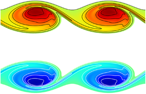
Figure 2. (a) Definition of the cylindrical reference frame together with a sketch of the initial condition of the simulation of the base flow. Here, the initial amplitude of the KH mode has been rescaled for sake of clarity. (b) Temporal evolution of the energy gain $G_E$ of the KH mode for $\alpha = 10$. The insets represent the azimuthal vorticity of the base flow $\Omega _{\theta }$ shown at times $t=5$, $t=T_s=10$ and $t=20$. The dash-dotted line stands for the energy growth predicted by the linear stability analysis.

The two-dimensional base flow consists of a time-evolving axisymmetric jet which undergoes the nonlinear development of the primary KH instability starting from the classical profile proposed by Michalke (Reference Michalke1971). The corresponding velocity $\boldsymbol {U}=[U_r,0,U_z]$ and pressure fields $P$ are computed on a meridian plane of dimension $[-r_{max}, r_{max}] \times [0, L_z]$ through a direct numerical simulation using a two-dimensional dealiased pseudo-spectral method described in detail in Joly, Fontane & Chassaing (Reference Joly, Fontane and Chassaing2005) and Joly & Reinaud (Reference Joly and Reinaud2007). In particular, we adopt a Fourier expansion in the streamwise direction and a Chebyshev collocation method for the radial direction (Khorrami, Malik & Ash Reference Khorrami, Malik and Ash1989). The Gauss–Lobatto collocation points defined in the Chebyshev space (${\mathcal {R}} \in [-1,1]$) are mapped into the physical space ($r \in [-r_{max}, r_{max}]$) thanks to a logarithmic mapping given by

(2.3)\begin{equation} r = a \tanh^{{-}1}{(b {\mathcal{R}})} \quad \textrm{with} \ b = \tanh{\left(\frac{r_{max}}{a}\right)}, \end{equation}

where the parameter $a$ controls the stretching of the collocation points. A free-slip boundary condition is imposed at the radial boundaries ($r = \pm r_{max}$) of the flow domain, while the flow is periodic in the streamwise direction.

As illustrated in figure 2(a), the initial condition used for the simulation of the base flow is the profile of Michalke (Reference Michalke1971) $\overline {\boldsymbol {U}}= [0,0,\overline {U}_z]$ given by

(2.4)\begin{equation} \overline{U}_z(r) = \frac 12 + \frac 12 \tanh \left[ \frac{\alpha}{4} \left( \frac{1}{r} - r \right)\right], \end{equation}

where $\alpha = \ell _0/\vartheta$ is the jet aspect ratio with $\vartheta$ the shear layer momentum thickness, perturbed by the most unstable mode obtained by the inviscid temporal linear stability analysis. The temporal modal analysis yields the phase velocity $c(\alpha )$ of the dispersion relation of the most unstable mode. We compensate for this phase velocity over the whole velocity field to keep the KH vortex ring at the centre of the Galilean reference frame. The saturation time $T_s$ of the primary instability depends on the initial amplitude of the KH mode $a_{KH}$, the Reynolds number ${Re}$ and the aspect ratio $\alpha$. The initial amplitude $a_{KH}$, defined as the square root of the ratio between the initial kinetic energy of the KH mode and the Michalke profile, is chosen small enough to ensure the existence of a linear phase of growth and its value is set so that the linear phase is the same for all cases, i.e. $\alpha T_s = 100$. The jet radius $\ell _0$ is set so that the most amplified KH mode corresponds to a wavenumber of $2 {\rm \pi}/L_z$. The radial extent of the domain is chosen large enough to ensure that the free-slip boundary condition has no influence on the nonlinear development of the flow, i.e. $r_{max}= 7 \ell _0$. For all simulations, we use a mesh of $512^{2}$ points, which has been checked to be large enough to ensure the convergence of the results. All the numerical settings for the homogeneous KH base flow fields are summarised in table 1.

Table 1. Main numerical parameters for the simulated homogeneous KH base flow fields: aspect ratio $\alpha$; jet radius $\ell _0$; phase velocity of KH mode $c$; maximum radius $r_{max}$; initial amplitude of the KH mode $a_{KH}$; and ratio $L_z/\ell _0$ between the domain streamwise extent and the jet radius and KH saturation time $T_s$.

Figure 2(b) shows the temporal evolution of the energy gain $G_E = E(t)/E(t_0)$ of the primary KH instability for $\alpha =10$. During the initial phase, the energy grows exponentially in time at a rate consistent with the growth rate predicted by the linear stability analysis. The nonlinear saturation of the mode occurs at $T_s=10$ and results in the unsteady roll-up of the axisymmetric shear layer into a KH vortex ring as illustrated by the contours of the azimuthal vorticity $\Omega _{\theta }$ in the insets of figure 2(b). In contrast with the plane shear layer case, the KH vortex does not exhibit a central symmetry with respect to the elliptical stagnation point, which is specific to the axisymmetry condition.

2.2. Optimisation problem

We now consider the temporal linear evolution of three-dimensional disturbances $[\boldsymbol {u},p]$ that are likely to grow over the incompressible KH vortex ring $[\boldsymbol {U},P]$. The governing equations (2.1) and (2.2) are linearised around the two-dimensional base flow:

(2.5)\begin{gather} \boldsymbol{\nabla} \boldsymbol{\cdot} \boldsymbol{u} = 0, \end{gather}

(2.6)\begin{gather}\frac{\partial \boldsymbol{u}}{\partial t} + \boldsymbol{U} \boldsymbol{\cdot} \boldsymbol{\nabla} \boldsymbol{u} + \boldsymbol{u} \boldsymbol{\cdot} \boldsymbol{\nabla} \boldsymbol{U} ={-} \boldsymbol{\nabla} p + \frac{1}{{Re}} \boldsymbol{\rm \Delta} \boldsymbol{u}. \end{gather}

We can write this linear system – referred to as the direct system – in the following compact form:

(2.7)\begin{equation} {{\boldsymbol{\mathsf{N}}}}_t \boldsymbol{\cdot} \boldsymbol{q} + {{\boldsymbol{\mathsf{N}}}}_c \boldsymbol{\cdot} \boldsymbol{q} + \frac{1}{{Re}}{{\boldsymbol{\mathsf{N}}}}_d \boldsymbol{\cdot} \boldsymbol{q} = 0, \end{equation}

where $\boldsymbol {q}=[\boldsymbol {u},p]$ is the direct variable vector and the three matrix operators are the temporal operator ${{\boldsymbol{\mathsf{N}}}}_t$, the operator of coupling between the base flow and the disturbance ${{\boldsymbol{\mathsf{N}}}}_c$ and the operator of viscous diffusion ${{\boldsymbol{\mathsf{N}}}}_d$, respectively.

The base flow being time-dependent and the dynamical system (2.7) non-normal, we resort to a non-modal stability analysis for which the temporal behaviour of the perturbation is not prescribed. Taking into account the streamwise periodicity and the axisymmetry of the base flow, the perturbation can be written in the form

(2.8)\begin{equation} [u_r,u_{\theta},u_z,p](r,\theta,z,t)= \frac{1}{2} \left([\tilde{u}_r,\tilde{u}_{\theta},\tilde{u}_z,\tilde{p}](r,z,t)\,\mathrm{e}^{\textrm{i}(\mu z+m\theta)} + \textrm{c.c.} \right), \end{equation}

where $m$ is the azimuthal wavenumber and $\mu$$\in [0, \, 1]$ the real Floquet exponent. As advocated in the introduction, the case where the base flow exhibits two-dimensional pairing is not considered here. Moreover, the works of Klaassen & Peltier (Reference Klaassen and Peltier1991) and Fontane & Joly (Reference Fontane and Joly2008) showed that the unstable modes of the stratified and the inhomogeneous mixing layers are only weakly sensitive to the Floquet exponent. For these reasons, we look for perturbations having the same streamwise periodicity as the base flow, i.e. $\mu = 0$.

Amongst all possible perturbations likely to develop within the KH vortex ring, we are interested in those maximising the growth of kinetic energy over a finite time interval $[t_0,T]$. The energy gain $G_E$ is defined as the ratio between the perturbation kinetic energy at the horizon time $T$ and the one at the injection time $t_0$:

(2.9)\begin{equation} G_E(T,t_0) = \frac{E(T)}{E(t_0)} = \frac{\Vert \boldsymbol{q}(T) \Vert_u}{\Vert \boldsymbol{q}(t_0) \Vert_u}, \end{equation}

where $\Vert \cdot \Vert _u$ stands for the seminorm associated with the conventional inner product and the kinetic energy (see appendix A for definition). In accordance with the pioneering work of Farrell (Reference Farrell1988), we define the optimal perturbation as the one reaching the maximal energy gain

(2.10)\begin{equation} {\mathcal{G}}_E(T,t_0) = \max_{\boldsymbol{q}(t_0)}\{G_E(T,t_0)\}, \end{equation}

over all the possible initial conditions $\boldsymbol {q}(t_0)$. To determine this optimal perturbation, we solve an optimisation problem with constraints (Gunzburger Reference Gunzburger2002) enforcing the disturbance to be a solution of the linearised Navier–Stokes equations (2.5) and (2.6). It can be converted to an optimisation problem without constraints by using the variational method of the Lagrange multipliers (see Luchini & Bottaro Reference Luchini and Bottaro1998; Corbett & Bottaro Reference Corbett and Bottaro2000, Reference Corbett and Bottaro2001). This approach involves the derivation of the so-called adjoint equations (Schmid Reference Schmid2007) associated with the direct system (2.5) and (2.6):

(2.11)\begin{gather} \boldsymbol{\nabla} \boldsymbol{\cdot} \boldsymbol{u}^{{\dagger}} = 0, \end{gather}

(2.12)\begin{gather}-\frac{\partial \boldsymbol{u}^{{\dagger}}}{\partial t} - \boldsymbol{U} \boldsymbol{\cdot} \boldsymbol{\nabla} \boldsymbol{u}^{{\dagger}} + \boldsymbol{u}^{{\dagger}} \boldsymbol{\cdot} \boldsymbol{\nabla} \boldsymbol{U}^{{\rm T}} = \boldsymbol{\nabla} p^{{\dagger}} + \frac{1}{{Re}} \boldsymbol{\rm \Delta} \boldsymbol{u}^{{\dagger}}, \end{gather}

where $\boldsymbol {u}^{\dagger }$ denotes the adjoint variable of the velocity field, $p^{\dagger }$ is the adjoint pressure and the superscript $^{{\rm T}}$ stands for the matrix transpose. The adjoint system can be also cast in the following compact form:

(2.13)\begin{equation} - {{\boldsymbol{\mathsf{N}}}}_t \boldsymbol{\cdot} \boldsymbol{q}^{{\dagger}} + {{\boldsymbol{\mathsf{N}}}}^{{\dagger}} _c \boldsymbol{\cdot} \boldsymbol{q}^{{\dagger}} + \frac{1}{{Re}}{{\boldsymbol{\mathsf{N}}}}_d \boldsymbol{\cdot} \boldsymbol{q}^{{\dagger}} = 0, \end{equation}

where $\boldsymbol {q}^{\dagger } = [\boldsymbol {u}^{\dagger },\,p^{\dagger }]$ is the adjoint variable vector. The negative sign before the temporal operator ${{\boldsymbol{\mathsf{N}}}}_t$ implies a backward-in-time integration of the adjoint equations. Here, ${{\boldsymbol{\mathsf{N}}}}^{\dagger } _c$ represents the adjoint coupling matrix operator between the base flow and the adjoint disturbance.

The identification of the optimal perturbation and the associated optimal energy gain ${\mathcal {G}}_E$, relies on an iterative optimisation algorithm described in detail in appendix A. The direct system (2.7) is advanced in time until the horizon time $T$, from an initial condition $\boldsymbol {q}(t_0)$ taken as a white noise. From the final direct state obtained at $T$, we compute the initial condition $\boldsymbol {q}^{\dagger }(T)$ for the adjoint system (2.13), before its integration backward-in-time to the injection time $t_0$. The resulting state is rescaled and used for the subsequent direct-adjoint integration. The optimisation loop is stopped when a 0.5 % convergence is achieved on the kinetic energy gain (see (A 5)). When compared with a perturbation obtained with a $0.1\,\%$ convergence rate, the $L_2$-norm of the difference between velocity fields remains below $2\,\%$ in relative value. Both direct and adjoint systems are integrated with the linearised version of the two-dimensional dealiased pseudo-spectral method used for the generation of the base flow. A rapid convergence of the optimisation problem is obtained in fewer than ten iterations.

We resort to the evolution equation for the energy growth rate of the perturbation $\sigma _E = (1/E) \,\mathrm {d}E/\mathrm {d}t$ to analyse the physical mechanisms associated with the energy growth of the optimal perturbations. This equation can be derived straightforwardly from the transport equation of the perturbation kinetic energy $E = \Vert \boldsymbol {q} \Vert _u$:

(2.14)\begin{align} \frac{\mathrm{d} E}{\mathrm{d} t} &= \underbrace{ - \int_{\mathcal{V}} u_r u_z \left( \frac{\partial U_r}{\partial z} + \frac{\partial U_z}{\partial r}\right) \mathrm{d} {\mathcal{V}}}_{{\Pi_{E_1}}} \underbrace{ - \int_{\mathcal{V}} \left( u^{2}_r \frac{\partial U_r}{\partial r} + u^{2}_{\theta} \frac{U_r}{r} + u^{2}_z \frac{\partial U_z}{\partial z} \right) \mathrm{d} {\mathcal{V}}}_{{\Pi_{E_2}}} \nonumber\\ &\quad \underbrace{ - \frac{1}{{Re}} \int_{\mathcal{V}} (\boldsymbol{\nabla} \boldsymbol{u} \boldsymbol{:} \boldsymbol{\nabla} \boldsymbol{u}^{T}) \,\mathrm{d} {\mathcal{V}}}_{{\Pi_{E_{\Phi}}}}, \end{align}

where the symbol $\boldsymbol {:}$ stands for the double contracted tensor product, $\Pi _{E_1}$ is the energy production/destruction due to the base flow shear, $\Pi _{E_2}$ the energy production/destruction due to the base flow strain field and $\Pi _{E_{\Phi }}$ the viscous dissipation of energy.

3.1. Optimal energy growth

We first consider the optimal perturbations of a round jet characterised by an aspect ratio $\alpha =10$ when injected at the initial time of the development of the base flow, i.e. $t_0 = 0$. Figure 3 displays the temporal evolution of the energy gain ${\mathcal {G}}_E$ of perturbations optimised for four horizon times between half the saturation time $T_s$ of the base flow KH wave and twice $T_s$, and for azimuthal wavenumbers ranging from $m=0$ to $m=5$. The time normalisation by $T_s$ will be used throughout the paper. The evolution of the energy gain of optimal perturbations growing over a diffusing unperturbed parallel jet with the Michalke profile, as obtained by Jimenez-Gonzalez et al. (Reference Jimenez-Gonzalez, Brancher and Martinez-Bazan2015), has been added for comparison. For the diffusing parallel jet, the energy curves are all superimposed indicating that increasing the horizon time does not modify the path but only raises the final energy gain reached by the disturbance. Therefore, the computation of the optimal perturbation for the largest horizon time explored is sufficient to access the energy gain evolution for any smaller $T$. The presentation of the optimal perturbations growing on a diffusing Michalke profile will be limited to that sole case in the following. Up to $t\sim T_s/2$, all perturbations follow the same energy growth while the still quasi-parallel base flow is in the linear phase of the KH instability. Even when optimised for long time horizons, the optimal perturbations thus exhibit the same primary growth as the one developing over a parallel jet. The influence of the nonlinear roll-up in the base flow is felt after $t\sim T_s/2$, corresponding to the onset of roll-up and of azimuthal vorticity concentration in the base flow, as illustrated in figure 2(b). This is the turning point where perturbations optimised for horizon times beyond the saturation time evolve from a primary to a secondary type. The onset of the nonlinear roll-up in the base flow yields the energy decrease of the axisymmetric optimal perturbation and bounds the energy growth of the helical and doubly helical ones. Conversely, for larger azimuthal wavenumbers, i.e. $m>2$, optimal perturbations developing over a diffusive parallel jet experience a substantial drop of energy, while perturbations optimised over a nonlinear KH roll-up benefit from a secondary phase of renewed though moderate energy growth.

Figure 3. Temporal evolution of the energy gain ${\mathcal {G}}_E$ for optimal perturbations growing over the roll-up of a nonlinear KH wave (black lines) and for the ones developing over a diffusing Michalke profile (grey lines) for six azimuthal wavenumbers: (a) $m=0$; (b) $m=1$; (c) $m=2$; (d) $m=3$; (e) $m=4$; and (f) $m=5$. The thick continuous line in panel (a) represents the temporal evolution of the energy gain of the primary KH mode, as displayed in figure 2(b). The symbols are located at the horizon time of each energy curve.

Figure 4(a) displays the final energy gain at horizon time ${\mathcal {G}}_E$ as a function of the horizon time $T$ extended to $3T_s$, for the same values of the azimuthal wavenumber. The optimal energy gain of perturbations growing over a diffusing Michalke profile has also been included in the background for reference. Whatever the azimuthal wavenumber, the energy gain grows on a similar trend until $T\approx 0.5 T_s$ up to a value of ${\mathcal {G}}_E \approx 10^{2}$. For all $m$, most of the perturbation energy growth is produced during this first phase. This initial period corresponds to the linear phase of the primary KH instability during which the axisymmetric shear layer has not rolled-up yet. After this initial phase, the energy of the axisymmetric disturbance $m=0$ continues to increase up to a maximal value obtained for a horizon time equal to the saturation time $T=T_s$ before decreasing monotonically when $T$ is increased further. The energy of the non-axisymmetric perturbations keeps on growing, although not always monotonically, when the horizon time is increased beyond $T\approx 0.5 T_s$. In particular, the helical mode is the only one to exhibit a monotonic energy growth. It stands as the so-called global optimal, the one displaying the largest energy growth over all wavenumbers up to $T\approx 2.5T_s$, when it is overtaken by the $m=2$ mode. If we consider $[T_s,2T_s]$ as the most favourable period for the development of secondary instabilities in real jets, the overall maximum energy gain corresponds to a helical perturbation whatever the horizon time, at least for the present values of the aspect ratio $\alpha$ and Reynolds number ${Re}$.

Figure 4. (a) Optimal energy gain ${\mathcal {G}}_E$ as a function of the normalised horizon time $T/T_s$ for different azimuthal wavenumbers at an injection time of $t_0 = 0$. (b) Influence of the azimuthal periodicity $m$ on the mean optimal growth rate $\sigma _m$ as a function of $T/T_s$. Dashed black lines correspond to the temporal evolution of (a) the energy gain $G_E$ and (b) the mean growth rate of the primary KH mode. Grey lines represent the optimal energy gain of perturbations growing over a diffusing Michalke profile.

In order to compare the growth efficiency of the various perturbations over the optimisation time frame, we consider the mean optimal energy growth rate $\sigma _m$ defined as follows:

(3.1)\begin{equation} \sigma_m = \dfrac{1}{T/T_s} \int_{0}^{T/T_s} \sigma_E (t) \, \mathrm{d} t = \dfrac{\ln\big[{\mathcal{G}}_E(T/T_s)\big]}{T/T_s}. \end{equation}

Figure 4(b) presents the evolution of $\sigma _m$ with the time ratio $T/T_s$ for all the azimuthal wavenumbers considered here. As $T$ increases, $\sigma _m$ decreases monotonically confirming that most of the energy growth occurs in the early times of the base flow evolution, i.e. before the nonlinear saturation of the KH wave into a roll-up. For the shortest horizon time considered here, $T=0.1T_s$, one can see that $\sigma _m$ increases monotonically with the azimuthal wavenumber $m$ (the largest is obtained for $m=5$), but immediately after (for $T \geq 0.2T_s$) the hierarchy changes and the helical mode progressively emerges as the global optimal until $T\approx 2.5T_s$ when it is overtaken by the double-helix perturbation ($m=2$) in accordance with the optimal energy gain ${\mathcal {G}}_E$ in figure 4(a).

We now focus on the spatial distribution of the energy during the time evolution in the interval $[0,T_s]$ of perturbations optimised for $T=T_s$, as displayed in figure 5.

Figure 5. Temporal evolution of the field of kinetic energy $E$ of optimal perturbations from $t=t_0$ to $t=T_s$ for various azimuthal wavenumbers. The energy is normalised by its current time maximum value and ten equally spaced coloured contour levels are used. Tick marks along the $r$ and $z$ axes correspond to the jet radius $\ell _0$. Dashed contours correspond to $20\,\%$ of the maximal absolute value of the base flow azimuthal vorticity $\Omega _{\theta }$.

At $t=t_0$, the optimal perturbations take the form of two elongated oblique layers whatever the azimuthal wavenumber $m$. These structures characterised by different azimuthal periodicity according to $m$ value are orientated along the direction of maximal compression of the base flow. During the time interval $[t_0,T_s/2]$, as the jet shear layer gradually rolls up into a vortex ring, these layers are progressively deformed under the action of the base flow mean shear in such way so as to be reoriented along the direction of base flow maximal stretching. This short-times evolution reflects the combination of Orr (Reference Orr1907) and lift-up (Ellingsen & Palm Reference Ellingsen and Palm1975) mechanisms, identified to be responsible for the transient energy growth of so-called ‘OL’ perturbations in plane shear layers (Arratia et al. Reference Arratia, Caulfield and Chomaz2013; Lopez-Zazueta et al. Reference Lopez-Zazueta, Fontane and Joly2016). The subsequent evolution of the axisymmetric $m=0$ perturbation for $t \geq T_s/2$ leads to a perturbation dipole located between the vortex core and the braid of the KH vortex ring. Once the shear-induced deformation has brought the initial energy growth due to the Orr-mechanism, the perturbation energy dipole is slowly dissipated but does not benefit from any three-dimensional relay mechanism for a secondary energy growth. For non-axisymmetric perturbations, the energy perturbation at the horizon time $T=T_s$ evolves progressively from a core-centred to a braid-centred distribution when $m$ is increased, as indicated by the location of the energy maximum in figure 5. At low $m$, the perturbation lies preferentially in the KH vortex core where the streamlines are locally elliptical and corresponds to an E-type instability while, at high $m$, the perturbation induces oscillations in the braid region where the streamlines are locally hyperbolic suggesting an H-type instability. This is analogous to the mixing layer (Arratia et al. Reference Arratia, Caulfield and Chomaz2013) and the parallel wake (Ortiz & Chomaz Reference Ortiz and Chomaz2011) where the secondary instabilities develop, respectively, on two-dimensional KH billows and on the von Kármán vortex street. Indeed higher azimuthal wavenumbers are associated with shorter azimuthal wavelengths and their associated perturbations are expected to grow in regions of the base flow where length scales are smaller. The hyperbolic region where the vorticity braid thickness decreases in time due to stretching thus naturally hosts the energy growth of large azimuthal wavenumber perturbations. Nevertheless, this scale selection between E-type and H-type perturbations with respect to $m$ is not exclusive since all the cases illustrated in figure 5 display energy in both regions, at least for the present values of azimuthal wavenumber $m$, aspect ratio $\alpha$ and Reynolds number ${Re}$.

The large amplification at short times, as seen in figure 4, is a typical feature of shear flows (Ortiz & Chomaz Reference Ortiz and Chomaz2011; Arratia et al. Reference Arratia, Caulfield and Chomaz2013; Garnaud et al. Reference Garnaud, Lesshafft, Schmid and Huerre2013a; Jimenez-Gonzalez et al. Reference Jimenez-Gonzalez, Brancher and Martinez-Bazan2015; Lopez-Zazueta et al. Reference Lopez-Zazueta, Fontane and Joly2016; Jimenez-Gonzalez & Brancher Reference Jimenez-Gonzalez and Brancher2017). The energy growth during this initial period is essentially due to base flow shear conversion as can be seen in figure 6 which presents the contributions to the temporal evolution of the energy growth rate according to (2.14) for perturbations optimised at $T=1.5 T_s$ from $m=0$ to $m=5$. As shown in figure 4(b) for the mean optimal growth rate, the energy growth is most efficient in the early times of the base flow evolution, i.e. $t \leq T_s$. The contribution of the base flow strain (term $\sigma _{E_2}$) remains very weak and the energy growth results essentially from the net balance between the base flow shear conversion $\sigma _{E_1}$ and the viscous dissipation $\sigma _{E_{\Phi }}$. This is very similar to the results of Arratia et al. (Reference Arratia, Caulfield and Chomaz2013) for the E-type instability (see their figure 7a) whose growth relies on both Orr and lift-up mechanisms. As detailed in the introduction, the Orr mechanism is a two-dimensional mechanism associated with changes in the area of the support of azimuthal vorticity patches under the action of the base flow mean shear. Given the constraint due to the Kelvin theorem that the circulation remains constant in the inviscid limit, any reduction in the support area increases azimuthal vorticity. It stems from a pure azimuthal perturbation vorticity $\omega _{\theta }$ and induces the amplification of both radial velocity $u_r$ and axial velocity $u_z$. On the other hand, the lift-up mechanism corresponds to the emergence of streaks of high and low streamwise velocity under the action of the base flow mean shear onto an initial perturbation made of an array of counter-rotating streamwise vortices. It is associated with an initial perturbation of axial vorticity $\omega _z$ which leads to large production of axial velocity streaks $u_z$. As explained by Farrell & Ioannou (Reference Farrell and Ioannou1993), the growth of the optimal perturbations in shear flows generally results from a synergistic combination of these two mechanisms: the radial perturbation velocity, fed by the Orr mechanism, enhances the streamwise rolls associated with streak production of the lift-up mechanism. The present case is no exception and the steep increase in energy in the early development of the perturbations observed in figure 6 is also due to this synergy. In this regard, we measure the relative contribution of each mechanism to the energy growth of the perturbation through the following ratios between the contribution of each component of velocity (vorticity) to the perturbation kinetic energy (enstrophy) at the injection time $t_0$:

(3.2a,b)\begin{equation} f_{u_i ^{2}} = \frac{\displaystyle\int_{{\mathcal{V}}} u_i ^{2} (t_0) \,\mathrm{d} {\mathcal{V}} }{E (t_0)}, \quad f_{\omega_i ^{2}} = \frac{\displaystyle\int_{{\mathcal{V}}} \omega_i ^{2} (t_0) \,\mathrm{d} {\mathcal{V}} }{Z (t_0)}, \end{equation}

where the subscript $i$ stands for the $i$th coordinate of the reference frame. Figure 7 shows these ratios as a function of the azimuthal wavenumber $m$.

Figure 6. Temporal evolution of the kinetic energy growth rate $\sigma _E$ and its different contributions according to (2.14) for the optimal perturbation with a horizon time $T=1.5 T_s$ and various azimuthal wavenumbers: (a) $m=0$; (b) $m=1$; (c) $m=2$; (d) $m=3$; (e) $m=4$; and (f) $m=5$.

Figure 7. Initial contribution to (a) the energy of each velocity component $f_{u_i ^{2}}$ and (b) the enstrophy of each vorticity component $f_{\omega _i ^{2}}$, as a function of the azimuthal wavenumber $m$. The horizon time is $T=1.5 T_s$.

In the axisymmetric case, only the radial and axial velocity components have non-zero value. The optimal perturbation thus takes advantage of a pure Orr mechanism ($\, f_{\omega _{\theta } ^{2}} = 1$ and $f_{\omega _{r} ^{2}} = f_{\omega _{z} ^{2}} = 0$). When the azimuthal wavenumber is increased, the contribution of the azimuthal velocity becomes more significant (so does the radial velocity) and the optimal perturbation gradually organises itself to benefit from both mechanisms. Figure7(b) shows that the two mechanisms contribute equally for $m=3$ ($\,f_{\omega _{\theta } ^{2}} \sim f_{\omega _{z} ^{2}}$) and then the lift-up becomes more efficient than the Orr mechanism for $m >3$ ($\,f_{\omega _{\theta } ^{2}} < f_{\omega _{z} ^{2}}$). Therefore, the combination of these two mechanisms ranges from a pure Orr-based growth for $m=0$ (lift-up is not active in two dimensions) to a predominance of lift-up for $m = 5$.

As already observed by Arratia et al. (Reference Arratia, Caulfield and Chomaz2013) and Lopez-Zazueta et al. (Reference Lopez-Zazueta, Fontane and Joly2016) in the homogeneous free shear layer, postponing the injection time $t_0$ does not change the physics but only reduces the efficiency of Orr and lift-up mechanisms, since the initial period during which these transient growth mechanisms are active is shorter. This is also the case here for the round jet.

3.2. Influence of the Reynolds number Re

In this section we investigate the influence of the Reynolds number ${Re}$ on the transient energy growth of secondary three-dimensional perturbations. Figure 8 displays the temporal evolution of the energy gain ${\mathcal {G}}_E$ for optimal perturbations obtained at ${Re}=10\,000$ compared with those calculated at ${Re}=1000$ for various horizon times and azimuthal wavenumber $m$. Increasing the Reynolds number results in a substantial increase of the energy gains for all perturbations. This is explained by two combined effects. First, the base flow exhibits sharper velocity gradients associated with higher levels of shear and the resulting energy production due to the base flow shear, i.e. term $\sigma _{E_{1}}$ in (2.14), is stronger. Second, the viscous dissipation $\sigma _{E_{\Phi }}$ is lowered with the increase of the Reynolds number.

Figure 8. Temporal evolution of the energy gain ${\mathcal {G}}_E$ of optimal perturbations at ${Re}=10\,000$ (black lines) and ${Re}=1000$ (grey lines) for various azimuthal wavenumbers: (a) $m=0$; (b) $m=1$; (c) $m=2$; (d) $m=3$; (e) $m=4$; and (f) $m=5$. The thick continuous lines in panel (a) represent the temporal evolution of the energy gain $G_E$ of the KH mode for the two cases. The symbols denote the optimisation time of each curve.

The temporal evolution from $t=t_0$ to the horizon time $T$, corresponding to the base flow saturation time $T_s$, of the spatial distribution of optimal perturbations kinetic energy is illustrated in figure 9 for azimuthal wavenumbers up to $m=5$. The optimal perturbations at initial time are very similar to those obtained for ${Re}=1000$, albeit the inclined layers are thinner. Their evolution during the time interval $[t_0,T_s/2]$, i.e. during linear phase of the KH mode growth in the base flow, results from shear induced deformation and the associated energy growth due to Orr and lift-up mechanisms. At horizon time, the energy is unevenly distributed between the core and the braid region of the KH vortex ring. With increasing azimuthal wavenumber, the transition from an E-type instability to an H-type instability is observed earlier versus the ${Re}=1000$ case. For $m \geq 2$, the energy growth lies preferentially in the braid region and the occurrence of an E-type response is even absent for $m \geq 5$. The increase in Reynolds number yields a thinner braid promoting the growth of perturbations with higher azimuthal wavenumbers. The scale selection underlying the outcome of E-type and H-type instabilities with optimal energy growth is steeper for larger Reynolds numbers.

Figure 9. Temporal evolution of the field of kinetic energy $E$ of optimal perturbations for ${Re}=10\,000$ from $t=t_0$ to $t=T=T_s$ for various azimuthal wavenumbers. Same conventions as in figure 5.

We analyse the structure of the initial perturbation by measuring the relative contribution $f_{u_i ^{2}}$ of velocity components to the energy and $f_{\omega _i ^{2}}$ of vorticity components to the enstrophy in the optimal perturbation at $t=t_0$ according to (3.2). Figure 10 displays the evolution of the structure of the initial perturbation with growing azimuthal wavenumber at ${Re}=10\,000$ together with those obtained for ${Re}=1000$. In the two-dimensional axisymmetric case, the optimal perturbation only takes advantage of the Orr mechanism, and, as $m$ increases, the Orr mechanism remains predominant over the lift-up mechanism, since $f_{\omega _{\theta } ^{2}} > f_{\omega _{z} ^{2}}$, at least up to $m=5$. Finally, increasing the Reynolds number results in larger energy gains and the promotion of higher azimuthal wavenumbers with no change in the nature of the underlying physical mechanisms.

Figure 10. Initial contribution to (a) the energy of each velocity component $f_{u_i ^{2}}$ and (b) the enstrophy of each vorticity component $f_{\omega _i ^{2}}$, as a function of the azimuthal wavenumber $m$ for ${Re}=10\,000$ (black lines) and ${Re}=1000$ (grey lines). The horizon time for the optimisation is $T=1.5 T_s$.

3.3. Round jet and free shear layer behaviours

Finally, we analyse the influence of the aspect ratio $\alpha$ on the optimal energy gain in order to study the effect of steepness of the initial jet velocity profile on the transient growth of secondary instabilities.

We first consider the optimal perturbations developing in a round jet characterised by an aspect ratio of $\alpha = 20$. In this case the shear layer momentum thickness is twice smaller than before compared with the jet radius, so that the cylindrical geometry does not have much effect on the flow development, which results to be comparable to a plane free shear layer. Figure 11(a) displays the final energy gain at horizon time ${\mathcal {G}}_E$ as a function of the normalised horizon time $T/T_s$ obtained up to $T=3T_s$ for the same values of azimuthal wavenumber as in the previous subsections. The optimal energy gain of perturbations growing over a diffusing unperturbed parallel jet has also been added in the background for reference. All amplification curves follow the same trend at the beginning, although perturbations characterised by higher azimuthal wavenumbers $m$ present initial energy growths slightly higher. As is the case with $\alpha = 10$, the essential part of the energy gain lies within the period of the linear evolution of the primary KH vortex ring during which the axisymmetric shear layer has not rolled-up yet. All disturbances developing during the unsteady base flow evolution towards the KH vortex ring feature a local maximum of the energy gain close to the saturation time $T_s$. For optimisation times larger than $T_s$, the energy gain decreases for $m \leq 2$ while it slightly increases for the other higher azimuthal wavenumber modes. The double-helix perturbation ($m=2$) remains the global optimal until a little before twice the KH saturation time where it is superseded by an $m=5$ disturbance. After such horizon time $T\approx 2T_s$, the flow would have bifurcated in the nonlinear regime to another state, so the helical and double-helix perturbations are likely to be the ones growing in the round jet at ${Re}=1000$. The increase in $\alpha$ associated with a scale reduction in shear layer momentum thickness $\vartheta$ promotes the emergence of a secondary mode of higher azimuthal periodicity, as is the case with the increase in Reynolds number.

Figure 11. Optimal energy gain ${\mathcal {G}}_E$ as a function of the normalised horizon time $T/T_s$ for different azimuthal wavenumbers at an injection time of $t_0 = 0$ for a base flow characterised by an aspect ratio of (a) $\alpha = 20$ and (b) $\alpha = 5$. Dashed black lines correspond to the temporal evolution of the energy gain $G_E$ of the corresponding primary KH mode. Grey lines represent the optimal energy gain of perturbations growing over a diffusing Michalke profile.

Now we consider the optimal perturbations developing in a round jet characterised by a small aspect ratio, i.e. $\alpha = 5$. Unlike in the previous case with $\alpha = 20$, the axisymmetry condition has a strong influence on the evolution of the base flow which forms a low-aspect-ratio vortex ring. This case corresponds to the round jet behaviour where the large scale geometry and the curvature of the shear layer are expected to make some difference to the secondary behaviour of the plane shear layer. The final energy gain at horizon time as a function of the horizon time is given in figure 11(b) for wavenumbers up to 5, together with the final energy gain of perturbations growing over a diffusing Michalke profile. After an initial phase of energy growth with similar trends as for larger $\alpha$, all perturbations see their energy decrease eventually with the horizon time. Only the helical perturbation exhibits a sustained energy growth with the horizon time. The $m=1$ perturbation is the global optimal and reaches levels of energy gains three orders of magnitude larger than the others for $T=3T_s$. It should be noted that, for this aspect ratio, the most unstable primary mode predicted by linear modal analysis is a helical KH mode (Jimenez-Gonzalez et al. Reference Jimenez-Gonzalez, Brancher and Martinez-Bazan2015) and the primary axisymmetric KH mode considered here is not likely to arise naturally in the round jet, unless forced appropriately. Furthermore, its energy growth is practically superimposed on the one of the optimal perturbation growing over a diffusing Michalke profile, as shown in figure 11(b). This optimal perturbation for $m=1$ taken at $t=2T_s$ is thus compared with the primary KH helical mode given by the modal stability analysis of Michalke profile in figure 12. The optimal helical perturbation over a low-$\alpha$ round jet proves to be very similar to the helical KH modal instability of the jet. This is confirmed by the correlation coefficients between the two fields which are close to unity: $0.97$ for the radial velocity component $u_r$, $0.94$ for the azimuthal velocity component $u_{\theta }$ and $0.87$ for the axial velocity component $u_z$. The axisymmetric KH vortex ring resulting from the KH instability in the base flow remains nested in the cylindrical shear layer during the nonlinear evolution of this low-Reynolds-number low-aspect-ratio jet. When compared with the $\alpha =20$ case, as illustrated in figure 13, it appears that the overall structure of the $\alpha =5$ base flow still resembles the one of the unperturbed jet. The small departure of this unsteady base flow from the parallel low aspect ratio one leaves it prone to transient and modal growth of helical perturbations, both in the first phase and in the long term.

Figure 12. Contours of the velocity field of (upper half-plane) the optimal helical perturbation optimised for $T=1.5T_s$ at a time of $t=2T_s$ and (lower half-plane) the primary KH helical mode obtained by the linear stability analysis. In both cases, the initial jet profile has an aspect ratio of $\alpha =5$. Contour levels are normalised by the maximal absolute value, solid (respectively, dashed) contours correspond to positive (respectively, negative) values. The thick continuous line in each panel represents the jet axis.

Figure 13. Temporal evolution of the azimuthal vorticity $\Omega _{\theta }$ for a base flow corresponding to an aspect ratio of $\alpha =5$ in the positive half-plane and $\alpha =20$ in the negative half-plane. The azimuthal vorticity is normalised by its current time maximum value. Tick marks along the $r$ axis correspond to the jet radius $\ell _0 (\alpha )$ and the thick continuous line in each figure represents the jet axis.

This marked difference between the free shear layer and the pure round jet behaviours also emerges from figure 14 which presents the optimal energy gain ${\mathcal {G}}_E$ as a function of the aspect ratio $\alpha$ obtained for a horizon time $T=1.5T_s$, which stands as an intermediate horizon time in the nonlinear phase of the base flow. The influence of $\alpha$ is displayed for the same values of azimuthal wavenumbers $m$, together with the results obtained for ${Re}=10\,000$. The dash-dotted line indicates the transition value of the aspect ratio, $\alpha =9.5$, below which the most amplified primary KH mode over the Michalke profile is the helical one, while it is the axisymmetric one above. On the left of this threshold, the gain values at $1.5T_s$ are spread over a wide range with a strong predominance of the helical perturbation. For ${Re}=1000$, the gain range between the helical perturbation and the less amplified one, i.e. $m=5$, broadens up to three orders of magnitude for $\alpha =5$. The same behaviour can be observed at ${Re}=10\,000$, even though in this case the axisymmetric perturbation is the least amplified of all optimal perturbations for all values of $\alpha$. On the other hand, the selection of the global optimal is less marked for higher aspect ratios $\alpha > 10$ with all the kinetic energy gains converging towards the same order of magnitude. The collapse of all final energy gain at $T=1.5T_s$ on one threshold with increasing aspect ratio is even more pronounced at ${Re}=10\,000$, with the sole exception of the axisymmetric perturbation ($m=0$). Therefore, the increase of the aspect ratio is associated with a lower selectivity of the azimuthal periodicity of the global optimal. This can be related to the experimental observation of Liepmann & Gharib (Reference Liepmann and Gharib1992) which found that, when the Reynolds number at the nozzle exit increases, i.e. when the shear layer thickness becomes thinner and $\alpha$ increases, the azimuthal wavenumber of secondary structures increases but the selection of the global optimal becomes weaker and less clear, as indicated by the error bars in their figure 15.

Figure 14. Optimal energy gain ${\mathcal {G}}_E$ in correspondence of a horizon time $T=1.5T_s$ as a function of the aspect ratio $\alpha$ at ${Re}=1000$ (black lines) and ${Re}=10\,000$ (grey lines), for different azimuthal wavenumbers $m$. The dash-dotted line represents the value of aspect ratio $\alpha =9.5$ below which the primary KH mode becomes helical.