3.1. Internal boundary layer

Following the surface transition, as the flow tries to adjust to the new wall condition, a distinct layer, called an IBL, forms within the overall boundary layer (see figure 1). As can also be seen in figure 1, the turbulent flow properties within the IBL could differ significantly from those of the upstream flow depending on the magnitude of the surface change. Similarly, a significant change in skin friction occurs following the surface transition, and most of the existing models require the growth of the IBL as an input to predict the evolution of the skin friction over the downstream surface. Thus, identifying the structure of IBLs under various surface transition conditions is of significant interest to accurately predict and model the behaviour of overall flow and skin friction.

A number of different methods have been proposed so far to detect IBLs (see Rouhi et al. Reference Rouhi, Chung and Hutchins2019). A great number of these methods are either based on the wall-normal variation of mean streamwise velocity (e.g. Elliott Reference Elliott1958; Antonia & Luxton Reference Antonia and Luxton1971a,Reference Antonia and Luxtonb; Bou-Zeid, Meneveau & Parlange Reference Bou-Zeid, Meneveau and Parlange2004), or the streamwise variation of either mean streamwise velocity (e.g. Andreopoulos & Wood Reference Andreopoulos and Wood1982) or its variance (e.g. Saito & Pullin Reference Saito and Pullin2014; Li et al. Reference Li, de Silva, Chung, Pullin, Marusic and Hutchins2021). With the present experimental data sets which cover both R $\rightarrow$ S and S $\rightarrow$ R surface transitions, we examined all of these methods. We observed that the methods based on the gradients in the streamwise direction, i.e. $\partial U /\partial x$ and $\partial u^2_{rms}/\partial x$, did not provide robust results for the identification of the IBLs, mainly due to the small gradients in the streamwise direction and comparable noise levels in PIV. The present data sets worked much better with the methods that are based on the wall-normal variation of the streamwise velocity, in particular with Elliott's (Reference Elliott1958) method, which is based on the logarithmic slope of $\partial U^+/\partial ln(y^+)$. With Elliott's (Reference Elliott1958) method, however, the wall-normal location to fit the logarithmic slope is not straightforward to determine. This is also the case with the method of Antonia & Luxton (Reference Antonia and Luxton1971a,Reference Antonia and Luxtonb), which is based on the inflection point in $U$ vs $y^{1/2}$ profile. This could explain some of the discrepancies in the literature for the power-law exponents describing the growth rates of IBLs (which is further discussed in the following).

To attain a more robust comparison among different surface transition cases in the present study, we employed a method that is based on the deviations in the $q=\partial U^+/\partial \ln (y^+)$ quantity (same quantity as in Elliott Reference Elliott1958) downstream the roughness change with respect to the upstream surface. That is, after forming a new wall-normal coordinate with respect to the local boundary layer thickness, $\delta$, for each streamwise location, we subtracted the local $q(x,y/\delta )$ quantity from the upstream mean of it, i.e. $\bar {q}(y/\delta )_{up}$, and then binarised the region that deviates from the upstream flow by $10\,\%$. Afterwards, we applied a power-law fit to the edge of the binarised region (based on the lower edge of the connected region in the wall-normal direction). Here, we used $10\,\%$ as a common threshold to determine the edge of the IBL, as this threshold works quite well for all the present surface transition cases. Less deviations from the upstream flow do not always result in a distinguished region for all the cases after binarisation (due to the variations in the noise level in PIV for each camera image as well as the relatively small deviations in $q$ for weak surface transition cases). With that, for the P24 $\rightarrow$ S surface transition case, we also used a weaker threshold, i.e. $5\,\%$ deviation relative to the upstream flow, as with this threshold we could obtain a similar IBL profile at each streamwise location with that in Li et al. (Reference Li, de Silva, Chung, Pullin, Marusic and Hutchins2021) (when both coordinates are normalised by $\delta _0$), where a similar surface transition, i.e. from P24 $\rightarrow$ S, is used. Note that they used a threshold of $\Delta (\overline {u^2} /U_\infty ^2)/\Delta \log _{10}(\hat {x}/\delta _0)=1\times 10^{-3}$.

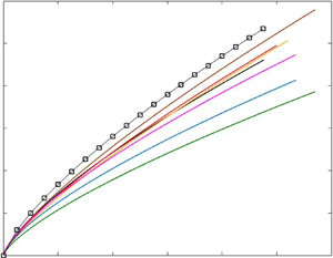
The resulting IBL profiles for all the surface transition cases in the present study are shown in figure 2(a) (except P24 $\rightarrow$ P36 and P36 $\rightarrow$ P24 cases: we could not obtain any distinguished IBL for these cases with the same method, as the magnitude of the surface transition hence the deviation in the flow quantity was very small). The power-law exponents ($b_o$) together with the constants ($A$) of the power-law fits to these IBLs, i.e. $\delta _{ibl}/\delta _0=A(x/\delta _0)^{b_o}$, on the other hand, are presented in figure 2(b). As can be seen in figure 2(a), when normalised by the upstream boundary layer thickness, the thicknesses of the IBLs at each streamwise location are quite similar for the P24 $\rightarrow$ S, P24 $\rightarrow$ P60 and P36 $\rightarrow$ S cases. The IBLs formed after the P60 $\rightarrow$ P24 and P60 $\rightarrow$ P36 transitions, on the other hand, are slightly thicker and thinner, respectively, compared with the former three R $\rightarrow$ S transition cases. For the P36 $\rightarrow$ P60 and P60 $\rightarrow$ S surface transition cases, however, the IBLs are significantly thinner compared with all other cases. From these profiles, it seems that for similar strength of the surface change (i.e. P24 $\rightarrow$ P60 & P60 $\rightarrow$ P24 and P36 $\rightarrow$ P60 & P60 $\rightarrow$ P36), slightly thicker IBLs are formed over the S $\rightarrow$ R transition cases compared with their R $\rightarrow$ S counterparts. This is consistent with the DNS and large-eddy simulation (LES) results of Rouhi et al. (Reference Rouhi, Chung and Hutchins2019) and Li & Liu (Reference Li and Liu2022), respectively, who also observed slightly thicker IBLs for the S $\rightarrow$ R surface transition. Note that in the former study, the surface transitions are from a rough sinusoidal surface to a smooth wall and vice versa, whereas in the latter study transition happens between two sinusoidal wavy surfaces.

Figure 2. (a) IBL profiles for all the surface transition cases, where a $10\,\%$ deviation in the $q=\partial U^+/\partial \ln (y^+)$ quantity relative to the upstream mean of it (i.e. $\bar {q}(y/\delta )_{up}$ over the upstream surface) is employed. Data shown in cyan with circle correspond to the power-law fit to the data of Li et al. (Reference Li, de Silva, Chung, Pullin, Marusic and Hutchins2021) with $A=0.094$ and $b_o=0.77$ ($\delta _{ibl}/\delta _0=A(x/\delta _0)^{b_0}$), whereas open square symbols correspond to the data for the P24 $\rightarrow$ S case with a weaker ($5\,\%$) threshold. (b) Filled symbols present the exponent, $b_o$, of the power-law fit to the experimental data for each surface transition case. Note that here each colour code represents a certain surface transition case, as shown in the legend in (a). Black square symbol corresponds to the result obtained with the weaker ($5\,\%$) threshold (corresponds to the IBL profile shown by open square symbols in a). In (c,d) power-law fit multiplicative coefficients, $A$, for all the cases are replotted for $| M |$ and $| M^*|$, respectively, as described in § 2. The error function fitted to the overall data in (d) (i.e. $A=1/2 \times [a+{\rm erf}((M^*-b)/(c\times sqrt(2)))]$ with $a=-0.83, b=-1.49$ and $c=1.1$) is also duplicated in (c) for comparison. Determined based on the error-function fit together with $|M|$ and $|M^*|$, the results for P24 $\rightarrow$ P36 and P36 $\rightarrow \,$P24 are shown in lilac and cyan respectively (c,d). Note that in (d), only the result for P24 $\rightarrow$ P36 is shown, as the result for P36 $\rightarrow \,$P24 is identical.

As can be seen from the distributions of the power-law fit exponents in (b), however, there is no significant trend with the magnitude of the surface change, and $b_0=0.75$ on average. This average value is very close to those obtained by Li et al. (Reference Li, de Silva, Chung, Pullin, Marusic and Hutchins2021) for a similar P24 $\rightarrow$ S surface transition case. Their power-law exponents are $b_0=0.77$ and $0.75$, for similar roughness Reynolds numbers $k_s^+={\sim }160$ and Reynolds numbers $Re_\tau =\sim 14\,000$, respectively (all are within fully rough flow regime and their IBL definitions are based on the streamwise variation of the turbulence intensity). In the present study, the surface transition cases cover both fully rough and transitionally rough flow regimes, i.e. $k_s^+(=16\unicode{x2013}81)$, and they are at much lower Reynolds numbers, i.e. $Re_\tau =1536\unicode{x2013}2532$. Despite these wide range of variations, a very similar power-law exponent shows no significant dependency on either $Re_\tau$ or $k_s^+$ in addition to the magnitude of the surface transition.

However, in the literature, different power-law exponents ranging between $b_0=0.2$ and $0.8$ have been reported (a great number of them either gather around 0.4 or asymptote to 0.8). Even with the same method, especially with the methods of Elliott (Reference Elliott1958) and Antonia & Luxton (Reference Antonia and Luxton1971a,Reference Antonia and Luxtonb), different studies have revealed different power-law exponents. This is mainly because the identification of the IBLs with these methods could be subjective (as it is not very straightforward to determine the location of the inflection points in the profiles). For instance, two recent studies, Li et al. (Reference Li, de Silva, Chung, Pullin, Marusic and Hutchins2021) and Li & Liu (Reference Li and Liu2022) have reported two different exponents, namely $b_0=0.78\unicode{x2013}0.81$ (for similar $Re_\tau -k_s^+$) and $b_0=0.25$, respectively, although both studies employed the same method of Antonia & Luxton (Reference Antonia and Luxton1971a,Reference Antonia and Luxtonb), who reported $b_0=0.43$. (These are all for R $\rightarrow$ S surface transition cases, where S is either a smooth wall or a smoother surface compared with the upstream surface.) On the other hand, the effect of using different methods on some of the results seem not that significant. In the present study, for instance, although we employed a different method from the methods used in Li et al. (Reference Li, de Silva, Chung, Pullin, Marusic and Hutchins2021) (who used both the method of Antonia & Luxton Reference Antonia and Luxton1971a,Reference Antonia and Luxtonb and the method based on the streamwise variation of turbulence intensity), we observed a similar power-law exponent on average, i.e. $b_0=0.75$. Moreover, this constant seems not to change significantly with the chosen threshold (see figure 2b). For instance, for the P24 $\rightarrow$ S case, instead of a $10\,\%$ threshold, using $5\,\%$ and $15\,\%$ thresholds increased and decreased the exponent by less than $1\,\%$ and $5\,\%$, respectively.

The multiplication constant of the power-law fit, however, could easily be affected by the chosen threshold that is used to distinguish the edge of the IBLs. As can be seen in figure 2 for the P24 $\rightarrow$ S case, although the power-law exponent is very similar for two different thresholds, the constant of the power-law fit could vary significantly depending on the selected threshold. On the other hand, similar to the power-law exponent, with the lower threshold ($5\,\%$) through which we obtained a similar IBL thickness with that in Li et al. (Reference Li, de Silva, Chung, Pullin, Marusic and Hutchins2021) at each streamwise location (see figure 2a), the resulting multiplication constant is found to be quite similar to the value reported by them ($A=0.100$ in the present study and $A=0.094\,(0.095)$ for the similar $k_s^+ (Re_\tau )$ data sets in their study where they used the streamwise variations in the turbulence intensity to detect the IBL). Note, however, that they found quite different values for $A$ with the method of Antonia & Luxton (Reference Antonia and Luxton1971a,Reference Antonia and Luxtonb), i.e. $A=0.062\,(0.059)$ for the similar $k_s^+ (Re_\tau )$ data sets.

When the multiplicative coefficients are compared for different surface transition cases in the present study, i.e. for different magnitudes of the surface change (figure 2c,d), two different behaviours are observed for $|M|$ and $|M^*|$ (see § 2). With $|M^*|$ (figure 2d), the coefficients are increasing with the magnitude of the surface transition for the R $\rightarrow$ S cases. The coefficients for the S $\rightarrow$ R transition cases, on the other hand, are similar to that of P24 $\rightarrow$ S. Overall, it is seen that all the results for the power-law fit coefficients could be represented by an error function (with $\delta _{ibl}=0$ for $M^*=0$ because there is no significant physical step change between the surfaces), i.e. $A=1/2 \times [a+{\rm erf}((M^*-b)/(c\times sqrt(2)))]$ with $a=-0.83$, $b=-1.49$ and $c=1.1$ (shown by purple solid line). When the same multiplicative coefficients are compared for $|M|$ in figure 2(c), the same error function seems to describe the behaviour of these coefficients for the fully rough cases and for the cases where the downstream surface is a smooth wall. For all other transitionally rough cases (all are rough-to-rough surface transitions), the coefficients are significantly higher than the fit. From these figures, it is clearly seen that for similar surface transition strengths, e.g. P36 $\rightarrow$ P60, P60 $\rightarrow$ P36 (and P60 $\rightarrow$ S in $c$) or P24 $\rightarrow$ P60 and P60 $\rightarrow$ P24, a thicker IBL is formed over the rougher downstream surface. This supports some of the previous models (see table 2 in the Appendix) which represent the growth of an IBL as a function of the roughness length of the downstream surface (rather than the upstream one). As can also be seen from these figures, surface transition strength also plays a role in the growth of IBLs. However, its effect decreases with increasing $|M^*|$ or $|M|$ (depending on the definition), and could asymptote to a single value as suggested by the present data.

In this section, we have examined the growth rates of IBLs for various R $\rightarrow$ S and S $\rightarrow$ R surface transition cases which cover both transitionally rough and fully rough flow regimes. In the following sections, we mainly discuss the response and the evolution of some of the flow properties (including sweep and ejection events) and coherent flow structures based on two-point spatial correlations which have remained relatively unexplored.

3.2. Velocity defect profiles and diagnostic plots

Mean streamwise velocity defect and diagnostic plots are frequently employed to assess the wall-similarity hypothesis of Townsend (Reference Townsend1956). According to the wall-similarity hypothesis, at sufficiently high Reynolds numbers the outer region does not feel the roughness effects on the wall. As reported recently by Gul & Ganapathisubramani (Reference Gul and Ganapathisubramani2021) for homogeneous surfaces, mean streamwise velocity defect profiles over the P24, P36 and P60 grit sandpapers (the same sandpapers as used in the present study) exhibit outer-layer similarity in the range of the Reynolds number $Re_\tau =1281\unicode{x2013}6317$ and roughness Reynolds number $k_s^+=14\unicode{x2013}195$. The diagnostic plots, on the other hand, hold wall similarity only for $k_s^+\geq 75\,(\Delta U^+\geq 7)$, as they showed. Thus, considering these results over these homogeneous surfaces, in this section we examine the behaviour of the mean streamwise velocity defect and diagnostic profiles under various R $\rightarrow$ S and S $\rightarrow$ R surface transitions (where flow regimes cover both transitionally and fully rough flows). In this section, we also briefly discuss the variance profiles for outer-layer similarity (for certain cases for brevity).

Figures 3 and 4 show the mean streamwise velocity defect profiles for the R $\rightarrow$ S and S $\rightarrow$ R cases, respectively, at various streamwise locations. Here, the wall-friction velocity of the upstream flow, i.e. $u_{\tau 1}$, is used for inner normalisation. As can be seen in these figures, velocity defect profiles close to the beginning of the surface change (up to $x/\delta _0=1$, considering the P24 $\rightarrow$ S case which has the strongest surface transition) preserve similarity very close to the wall. This shows that a significant part of the boundary layer is not affected by the surface change closer to the surface transition. However, with increasing streamwise distance from the surface transition, as the effects of the new wall condition propagate towards the interior of the boundary layer, i.e. with the growth of the IBL, the defect profiles deviate further from the upstream condition. The profiles become lower than the upstream case for the R $\rightarrow$ S cases, whereas they become higher for the S $\rightarrow$ R cases. This is consistent with the expected behaviour of the skin friction (and accordingly the wall-friction velocity) downstream of the surface change (which undershoots and overshoots their upstream counterparts over the downstream surface after the surface transition for the R $\rightarrow$ S and S $\rightarrow$ R cases, respectively).

Figure 3. Streamwise velocity defect profiles, $(U_\infty -U)^+$, for the R $\rightarrow$ S cases at various streamwise locations: (a) P24 $\rightarrow$ S, (b) P36 $\rightarrow$ S, (c) P60 $\rightarrow$ S, (d) P24 $\rightarrow$ P60, (e) P36 $\rightarrow$ P60 and ( f) P24 $\rightarrow$ P36. Here, for each streamwise location, the profiles are averaged over ${\sim }0.2\delta _0$, and for the inner normalisation wall-friction velocity of the upstream flow, i.e. $u_{\tau 1}$ is used. Dashed blue lines are mean profiles over the upstream part before the transition, i.e. between $x/\delta _0=-2$ and $x/\delta _0=-0.05$.

Figure 4. Streamwise velocity defect profiles, $(U_\infty -U)^+$, for the S $\rightarrow$ R cases at various streamwise locations: (a) P60 $\rightarrow$ P24, (b) P60 $\rightarrow$ P36 and (c) P36 $\rightarrow$ P24. Here, for each streamwise location, the profiles are averaged over ${\sim }0.2\delta _0$, and for the inner normalisation wall-friction velocity of the upstream flow, i.e. $u_{\tau 1}$ is used. Dashed blue lines are mean profiles over the upstream part before the transition, i.e. between $x/\delta _0=-2$ and $x/\delta _0=-0.05$.

To collapse these defect profiles, the scaling friction velocity at each streamwise location should also vary in the wall-normal direction between $u_{\tau 2}(x)$, which is the local condition, to $u_{\tau 1}$, which is the upstream condition. Here, we would like to note that although the defect profiles deviate more from the upstream profiles with streamwise distance for the cases that have stronger surface transition, there is no clear observable trend on the effect of the magnitude of the surface transitions on these deviations.

Similar behaviour was also observed in the variance of the streamwise and wall-normal velocities (when normalised by $u^2_{\tau 1}$), as presented in figure 5. This clearly shows that above the IBL, these second-order flow properties remain self-similar with those of the upstream flow, as the effects of the new surface conditions have not yet reached that part of the flow.

Figure 5. Variance of the streamwise ($\overline {u^2}/u^2_{\tau 1}$, dotted lines) and wall-normal ($\overline {v^2}/u^2_{\tau 1}$, solid lines) velocities, normalised by the upstream wall-friction velocity, $u_{\tau 1}$: (a) P24 $\rightarrow$ S, (b) P36 $\rightarrow$ S, (c) P36 $\rightarrow$ P60 and (c) P60 $\rightarrow$ P24. For each streamwise location, the profiles are averaged over ${\sim }0.2\delta _0$, and same colour code is applied here as in figures 3 and 4.

The effect of the surface transition is also visible in the diagnostic plots, where the turbulence intensity (e.g. $\sqrt {\overline {u^2}}/U$) profiles are plotted against $U/U_\infty$ (see figures 6 and 7 for the R $\rightarrow$ S and S $\rightarrow$ R cases, respectively). Similar to the above defect profiles, for the R $\rightarrow$ S cases (except P24 $\rightarrow$ P36), the deviations from the upstream profile occur first close to the wall after the surface change, and these deviations cover a larger wall-normal distance with the growth of the IBL over the downstream surface. This gradual change in the diagnostic profiles is not observed in the S $\rightarrow$ R cases. In addition, different from its R $\rightarrow$ S counterpart, the diagnostic profile at $x/\delta _0=1$ for the P60 $\rightarrow$ P24 transition case seems to undershoot the upstream equilibrium profile (except the region very close to the wall), and the affected wall-normal distance is greater than the corresponding IBL thickness at this streamwise location. For all the surface transition cases, however, the profiles farthest away from the step change approach to those represented by dotted black lines (for rough downstream surface) or black lines with filled circles (for smooth downstream surface). Here, dotted black lines correspond to the mean profiles over a streamwise fetch of $-2\delta _0$ and $-0.05\delta _0$ (before the location of the surface change) assuming the whole test section is covered homogeneously by the downstream surface. Data shown by black lines with filled circles, on the other hand, represent the experimental data of Hutchins et al. (Reference Hutchins, Monty, Ganapathisubramani, Ng and Marusic2011). For comparison, here, we also show the smooth-wall asymptote of Alfredsson, Orlu & Segalini (Reference Alfredsson, Orlu and Segalini2012) (black dashed lines). The profiles for the R $\rightarrow$ S cases show that even if the upstream flow before the step change is fully rough (which is the case for the transitions where upstream surface is P$24$), the diagnostic profiles within the IBL could have a transitionally rough or hydraulically smooth flow behaviour depending on the roughness properties of the downstream surface. For the S $\rightarrow$ R cases, on the other hand, the diagnostic profiles (within the IBLs) become more close to fully rough behaviour (except very close to the surface transition for the P60 $\rightarrow$ P24 case), and the equilibrium profile is reached much quicker compared with their R $\rightarrow$ S counterparts.

Figure 6. Streamwise turbulence intensities, $\sqrt {\overline {u^2}}/U$, plotted against the mean velocity normalised by the free stream velocity, $U/U_\infty$, for the R $\rightarrow$ S cases at various streamwise locations: (a) P24 $\rightarrow$ S, (b) P36 $\rightarrow$ S, (c) P60 $\rightarrow$ S, (d) P24 $\rightarrow$ P60, (e) P36 $\rightarrow$ P60 and ( f) P24 $\rightarrow$ P36. Here, each profile is averaged over ${\sim }0.2\delta _0$. Dashed blue lines are mean profiles over the upstream part before the transition, i.e. between $x/\delta _0=-2$ and $x/\delta _0=-0.05$. These profiles are also denoted by dotted black lines for the corresponding downstream surfaces; for instance, the dotted black line in (d) corresponds to the dashed blue line in (c). Dashed black lines, on the other hand, correspond to the smooth wall asymptote of Alfredsson et al. (Reference Alfredsson, Orlu and Segalini2012), whereas black lines with circles correspond to the experimental data of Hutchins et al. (Reference Hutchins, Monty, Ganapathisubramani, Ng and Marusic2011).

Figure 7. Streamwise turbulence intensities $\sqrt {\overline {u^2}}/U$ plotted against the mean velocity normalised by the free stream velocity, $U/U_\infty$, for the S $\rightarrow$ R cases at various streamwise location: (a) P60 $\rightarrow$ P24, (b) P60 $\rightarrow$ P36 and (c) P36 $\rightarrow$ P24. Dashed blue lines are mean profiles over the upstream part before the transition, i.e. between $x/\delta _0=-2$ and $x/\delta _0=-0.05$. These profiles are also denoted by dotted black lines for the corresponding downstream surfaces; for instance, the dotted black line in (b) corresponds to the dashed blue line in (c).

For the P24 $\rightarrow$ P36 and P36 $\rightarrow$ P24 cases, however, because the steady-state diagnostic profiles over the homogeneous P36 and P24 surfaces are very close to each other, the effect of the surface transition (independent of the magnitude of the surface transition) is not expected to be visible in these diagnostic plots. We would like to note here that using the above diagnostic profiles for the R $\rightarrow$ S transition cases (except P24 $\rightarrow$ P36), we also identified the IBLs and obtained similar results as in figure 2.

3.3. Sweep and ejection events

In this section, we examine the evolution of the ejection, $Q_2$, and sweep, $Q_4$, events over the R $\rightarrow$ S and S $\rightarrow$ R cases. Note that previously no significant differences were observed in the contribution of the sweep and ejection events to the overall turbulent shear stress, when the results for different grit sandpapers (i.e. P24, P36 and P60; homogeneous surfaces) are compared for a range of $Re_\tau (1281\unicode{x2013}6317)$ and $k_s^+ (14\unicode{x2013}195)$ (Gul & Ganapathisubramani Reference Gul and Ganapathisubramani2021). Similar to that study, for the quadrant analysis, we employed the parabolic hole approach of Lu & Willmarth (Reference Lu and Willmarth1973) with hyperbolic hole size $H=1$. (Note that similar results were also found with $H=0$.) The resulting $Q_2$ and $Q_4$ profiles (averaged over a streamwise distance of ${\sim }2\delta _0$) for various streamwise locations relative to the location of the surface change are presented in figure 8 for selected cases (for brevity).

Figure 8. Contribution of the ejection ($Q_2$, dashed lines) and sweep ($Q_4$, solid lines) events to the overall turbulent shear stress at various streamwise location. Blue, red, yellow, green, magenta and black lines correspond to the data averaged over $x\sim (-2\unicode{x2013}0)\delta _0$, $(0\unicode{x2013}2)\delta _0$, $(2\unicode{x2013}4)\delta _0$, $(4\unicode{x2013}6)\delta _0$, $(6\unicode{x2013}8)\delta _0$ and $(8\unicode{x2013}10)\delta _0$, respectively: (a) P24 $\rightarrow$ S, (b) P60 $\rightarrow$ S, (c) P24 $\rightarrow$ P60, (d) P36 $\rightarrow$ P60, (e) P60 $\rightarrow$ P24 and ( f) P36 $\rightarrow$ P24.

In figure 8(a), it can be seen that for the P24 $\rightarrow$ S transition case, the contribution of the ejection and sweep events are decreasing and increasing, respectively, within the IBL, as the flow accelerates over the smooth surface. Beyond $y/\delta =0.5$, however, no clear differences are observed similar to the other flow quantities as discussed in § 3.2. As the magnitude of the surface transition decreases, the changes in $Q_2$, and $Q_4$ events diminish in strength for the other smooth wall cases (i.e. P36 $\rightarrow$ S and P60 $\rightarrow$ S), and the equilibrium state is reached earlier. For the other R $\rightarrow$ S cases (i.e. when the downstream surface is also rough), however, it seems that the differences in the $Q_2$ and $Q_4$ events are not significant, similar to our previous findings over the same sandpapers without any surface change (Gul & Ganapathisubramani Reference Gul and Ganapathisubramani2021). Thus, the differences in the contribution of the $Q_2, Q_4$ events for these R $\rightarrow$ S cases could be due to the smooth wall where the absence of rough elements mitigate (enhance) the $Q_2$ ($Q_4$) events.

For the P60 $\rightarrow$ P24 case (figure 8e), on the other hand, the contribution of the $Q2$ ($Q4$) events first undershoots (overshoots) just after the surface change in the vicinity of the wall, and then overshoots (undershoots) until it reaches the upstream equilibrium profile, as the flow decelerates over the downstream surface. This behaviour becomes less distinguished as the magnitude of the surface transition decreases, and as can be seen in figure 8( f) from the P36 $\rightarrow$ P24 case, finally, no differences are observed. These results suggest that when flow transitions from a rough surface with a small roughness Reynolds number (i.e. $k_s^+$) to a much rougher surface, some changes in the contribution of sweep and ejection events could occur downstream of the step change, but finally initial equilibrium profiles would be reached after some streamwise fetch.

As these profiles suggest, the contribution of the sweep and ejection events could be affected significantly by the sudden surface change, and the nature of the response of these events to the surface change depends on both the magnitude and the nature of the surface transition, i.e. whether it is rough-to-smooth, rough-to-smoother or rough-to-rougher.

3.4. Spatial structures

Different from the §§ 3.2 and 3.3, where we examine the effect of the strength as well as the nature of surface transition on various turbulence quantities, in this section, we investigate the evolution of the spatial structures downstream the surface transition. This is done by comparing the large-scale structures that are present in the flow through two-point spatial correlations over a streamwise fetch of $2\delta _0$ (ignoring non-homogeneity over each streamwise fetch). The streamwise ($l_x$) and wall-normal ($l_y$) lengths of the average flow structures were determined based on $R_{uu,vv}=0.5$. Here, $R_{uu}$ and $R_{vv}$ are the correlation coefficients for the streamwise and wall-normal velocity fluctuations, i.e. $u$ and $v$, respectively (see Gul & Ganapathisubramani (Reference Gul and Ganapathisubramani2021) for the two-point spatial correlation formula as well as for the details of the analysis). The resulting streamwise and wall-normal lengths of the correlation coefficients for four different reference wall locations (i.e. $y/\delta$) are shown in figure 9 for P24 $\rightarrow$ P60 (solid lines with filled symbols) and for the inverse transition case, i.e. P60 $\rightarrow$ P24 (dashed lines with open symbols). Note that in these figures, we considered four different streamwise fetches relative to the step change, namely $(-2\unicode{x2013}0)\delta _0$ (shown in blue), $(0\unicode{x2013}2)\delta _0$ (shown in red), $(6\unicode{x2013}8)\delta _0$ (shown in magenta) and $(8\unicode{x2013}10)\delta _0$ (shown in black).

Figure 9. Wall-normal ($l_y$) and streamwise ($l_x$) lengths of two-point correlation coefficients ($R$) of streamwise velocity ($u$) and wall-normal velocity ($v$) fluctuations (i.e. $R_{uu}$ and $R_{vv}$, respectively). Solid lines with filled symbols correspond to the results for the surface transition case P24 $\rightarrow$ P60, whereas dashed lines with open symbols represent the results for P60 $\rightarrow$ P24. Same colour code as in figure 8 applies here, i.e. blue, red, magenta and black profiles correspond to the results obtained over a streamwise fetch of ${\sim} (-2\unicode{x2013}0)\delta _0$, $(0\unicode{x2013}2)\delta _0$, $(6\unicode{x2013}8)\delta _0$ and $(8\unicode{x2013}10)\delta _0$, respectively.

As can be seen in figure 9(a,c) for the P24 $\rightarrow$ P60 case, the wall-normal length of both correlation coefficients, i.e. $l_{y,uu}$ and $l_{y,vv}$, increases as the flow develops over the downstream surface. That is the average flow structures become thicker in the wall-normal direction, as the flow accelerates downstream of the surface after the transition. For the reverse transition case, i.e. P60 $\rightarrow$ P24 (figure 9a,e), however, flow deceleration over the second surface causes the average flow structures to become thinner in the wall-normal direction. There is also a clear decrease in the streamwise length of the average flow structures (both $l_{x,uu}$ and $l_{x,vv}$) for the P60 $\rightarrow$ P24 case (figure 9b, f). Although the differences are not that significant for the P24 $\rightarrow$ P60 case for the streamwise length of the correlation coefficients for the streamwise velocity fluctuations, it is seen that both correlation coefficients become more elongated in the streamwise direction for this case, as the flow accelerates over the smoother surface (see figure 9b,d). Note that previously the DNS results of Ismail et al. (Reference Ismail, Zaki and Durbin2018) (where flow transitions from a rib-roughened surface to a smooth wall in a turbulent channel flow) showed that the streamwise integral length scale of streamwise velocity fluctuations near the step change (i.e. within $x/\delta \leq 0\unicode{x2013}2.57$) are greater than the streamwise length scales of the upstream flow at various reference wall-normal locations up to $y/\delta =0.2$. Between $y/\delta =\sim 0.25$ and $0.75$, however, these length scales gradually become smaller with the streamwise distance (up to $x/\delta =2.57$). Although this near-wall region behaviour is consistent with the present results in figure 9(b) (for the R $\rightarrow$ S case), the differences between these two studies away from the wall could be explained by the differences in the flow geometries.

In this section, we also investigated the evolution of the low- and high-speed structures for the same surface transition cases. To do that, we conditioned the two-point correlation analysis on the low- and high-speed events ($u<0$ and $u>0$, respectively). The resulting wall-normal ($l_{y,uu}$) and streamwise ($l_{x,uu}$) lengths of these events are presented in figure 10. Here, for brevity we only present the results for two different streamwise fetches relative to the location of the surface change, i.e. $(-2\unicode{x2013}0)\delta _0$ and $(8\unicode{x2013}10)\delta _0$. Results shown by solid lines with filled symbols correspond to the low-speed events, whereas the resulting profiles for the high-speed events are presented by dotted lines with open symbols. As can be seen from these figures, similar to the average flow structures, the peaks of the correlation coefficients conditioned on the low- and high-speed events become thicker and more elongated in the wall-normal and streamwise directions, respectively, as the flow accelerates over the smoother surface (i.e. for the P24 $\rightarrow$ P60 transition case). For the reverse transition case (i.e. P60 $\rightarrow$ P24), however, these structures (both low- and high-speed events) become thinner and shorter in the wall-normal and streamwise directions, respectively. The changes in the lengths of these structures seem to be quite similar for both events, when the results for these two different streamwise fetches are compared. These results are consistent with figure 11 of Li & Liu (Reference Li and Liu2022), which shows that the iso-surfaces of both low- and high-speed structures are bigger after the flow transitions over a smoother surface. Note that their study is based on LES over two sinusoidal wavy surfaces with $| M |=1.06$.

Figure 10. Wall-normal ($l_y$) and streamwise ($l_x$) lengths of two-point spatial correlation coefficients of streamwise velocity ($u$) and wall-normal velocity ($v$) fluctuations (i.e. $R_{uu}$ and $R_{vv}$, respectively). Here, the correlations are conditioned on either low-speed events, i.e. $u<0$ (filled symbols with solid lines), or high-speed events, i.e. $u>0$ (open symbols with dotted lines). Data shown in blue and black correspond to the results over a streamwise fetch of ${\sim} (-2\unicode{x2013}0)\delta _0$ and $(8\unicode{x2013}10)\delta _0$, respectively, relative to the location of the surface change. In (a,b) results for the P24 $\rightarrow$ P60 transition case are presented, whereas in (c,d) results for the inverse transition case, i.e. P60 $\rightarrow$ P24, are shown.

3.5. Skin friction development model

In transportation industry, skin friction constitutes a significant portion of the overall drag, e.g. up to $90\,\%$ in shipping (Schultz et al. Reference Schultz, Bendick, Holm and Hertel2011) and $50\,\%$ in aviation (Spalart & McLean Reference Spalart and McLean2011). Hence, accurate prediction of overall skin friction is of significant interest. However, the existing predictive models mainly assume homogeneous surface topography, which is not the case in many of the engineering applications and therefore incorrectly estimates the overall drag. As can be seen in various literature (e.g. Antonia & Luxton Reference Antonia and Luxton1971a,Reference Antonia and Luxtonb; Efros & Krogstad Reference Efros and Krogstad2011; Hanson & Ganapathisubramani Reference Hanson and Ganapathisubramani2016; Li et al. Reference Li, de Silva, Rouhi, Baidya, Chung, Marusic and Hutchins2019), skin friction undergoes a sudden change when exposed to surface inhomogeneity, which even undershoots (overshoots) the value of the equilibrium state of the downstream surface after rough-to-smooth (smooth-to-rough) streamwise surface transitions. Moreover, skin friction is crucial to determine wall-friction velocity which is one of the fundamental scaling parameters in wall turbulence. Hence, it is very important to accurately predict the development of skin friction over inhomogeneous surfaces. In this section, we explore the utility of a given model based on the large dataset obtained in this study.

A number of methods have been proposed so far, and among them Elliott's (Reference Elliott1958) model seems one of the simplest and reasonably accurate. For instance, the oil-film measurements of Li (Reference Li2020) for the P24 $\rightarrow$ S surface transition shows that Elliott's (Reference Elliott1958) model (which models the flow within and outside the IBL with two logarithmic profiles) predicts the behaviour of the flow quite well (within $3\,\%$ accuracy for all the cases investigated where $Re_\tau =7100\unicode{x2013}21\,000$ and $k_s^+=111\unicode{x2013}228$). Similarly, when Elliott's (Reference Elliott1958) model is applied to the rough (grit surface)-to-smooth surface transition data of Hanson & Ganapathisubramani (Reference Hanson and Ganapathisubramani2016) (where $M=-3.4$), it is seen that the model underestimates the experimental data (obtained with Preston tube) within $5\,\%$ (see figure 11a). However, as can be seen from the same figure, the prediction (relative to the Preston tube measurements) becomes worse for their mesh surface-to-smooth wall transition case where $M=-5.1$. Considering these comparisons, Elliott's model seems to provide accurate results within $5\,\%$ for $|M| \leqslant 3.4$ (for rough-to-smooth transition cases). Hence, for our surface transition cases, where $| M |<3$, also considering the similarity of our strongest surface transition case with that in Li (Reference Li, de Silva, Rouhi, Baidya, Chung, Marusic and Hutchins2019) (i.e. P24 $\rightarrow$ S), Elliott's (Reference Elliott1958) model is expected to yield results for the wall-friction velocity within $3\,\%$. However, we would like to note here that some of the present surface transition cases are in the transitionally rough flow regime, also include S $\rightarrow$ R transition cases, both of which have been subject of limited number of investigations. Thus, further studies are needed to verify the results for these cases.

Figure 11. (a) Wall-friction velocity over the downstream surface relative to the upstream value of it, i.e. $u_{\tau,2}/u_{\tau,1}$, for all the R $\rightarrow$ S transitions. Here, the inverse of this ratio, i.e. $u_{\tau,1}/u_{\tau,2}$, is presented for the S $\rightarrow$ R cases to compare the results with their R $\rightarrow$ S counterparts. All the data were obtained using the model proposed by Elliott (Reference Elliott1958) based on the experimental data sets of Gul & Ganapathisubramani (Reference Gul and Ganapathisubramani2021), together with a (modified) logarithmic fit. The magnitude of the surface change is $M[=\ln (y_{02}/y_{01})]$, where $y_{02}$ corresponds to the roughness length determined at the farthest location beyond the surface change. For further comparison, the experimental data of Hanson & Ganapathisubramani (Reference Hanson and Ganapathisubramani2016) for grit-to-smooth ($M=-3.4$, shown by filled square symbols) and mesh-to-smooth ($M=-5.1$, shown by open square symbols) are presented together with the results obtained with Elliott's (Reference Elliott1958) model for these two cases (solid and dotted lines, respectively). Inset shows the milder surface transition cases for comparison. (b) Resulting $u_{\tau,2}/u_{\tau,1}$ data at a streamwise distance of $x/\delta _0=9.5$ beyond the surface transition. In (a,b) the data shown in black, red, yellow, blue, green, lilac, cyan, magenta and brown correspond to the P24 $\rightarrow$ S, P36 $\rightarrow$ S, P24 $\rightarrow$ P60, P36 $\rightarrow$ P60, P60 $\rightarrow$ S, P24 $\rightarrow$ P36, P36 $\rightarrow$ P24, P60 $\rightarrow$ P36 and P60 $\rightarrow$ P24, respectively. All the R $\rightarrow$ S data (including some of the literature) together with inverse values of their S $\rightarrow$ R counterparts are shown in the inset.

Elliott's (Reference Elliott1958) model (originally developed for atmospheric boundary layers) basically represents the mean velocity profile, $U$, within the IBL, i.e. $y<\delta _{ibl}$, and the unaffected flow above it, i.e. $y>\delta _{ibl}$, with two logarithmic profiles

(3.1) \begin{equation} U(y) = \begin{cases} \dfrac{u_{\tau1}}{\kappa}\ln(y/y_{01}), & y>\delta_{ibl},\\ \dfrac{u_{\tau2}}{\kappa}\ln(y/y_{02}), & y<\delta_{ibl}. \end{cases} \end{equation}

Here, $\delta _{ibl}$ is the local IBL thickness, as determined in § 3.1 for all the surface transition cases. Note that for the weak surface transition cases, i.e. P24 $\rightarrow$ P36 and P36 $\rightarrow$ P24, the error-function fit in figure 2(d) is used to determine the local IBL (as all the data seem to be represented by an error-function fit). Roughness length of the homogeneous upstream surfaces, i.e. $y_{01}$, was determined based on the experimental data of Gul & Ganapathisubramani (Reference Gul and Ganapathisubramani2021) for all the sandpapers. The roughness length of the downstream surfaces, i.e. $y_{02}$, on the other hand, were determined from $y_{02}=({\nu }/{u_{\tau 2}}){\rm e}^{-A \kappa }$ and $y_{02}=({\nu }/{u_{\tau 2}}){\rm e}^{-\kappa (A-\Delta U^+)}$ for the smooth and rough walls, respectively (except P24 $\rightarrow$ P60 and P24 $\rightarrow$ P36 cases, for which a fully rough relation, i.e. $y_{02}=k_s\exp (-\kappa A'_{FR})$, was used). As discussed in § 2, the values of $u_{\tau 2}$ and $\Delta U^+$ were obtained at the farthest location from the surface change through logarithmic and modified logarithmic fits for the smooth and rough walls, respectively. Hence, in this section $| M|$ is used to quantify the magnitude of the surface transition (see § 2) and accordingly to compare the results with the existing literature. The resulting profiles for the wall-friction velocity over the downstream surface, i.e. $u_{\tau,2}$, with respect to the upstream value, i.e. $u_{\tau,1}$ are presented in figure 11(a). Note that for the S $\rightarrow$ R cases, the inverse of $u_{\tau,2}/u_{\tau,1}$ is plotted for comparison. Also here in this figure, the experimental results (Preston tube measurements) of Hanson & Ganapathisubramani (Reference Hanson and Ganapathisubramani2016) for grit-to-smooth and mesh-to-smooth surface transition cases are shown together with the results produced using Elliott's (Reference Elliott1958) model (solid and dotted lines, respectively) for the surface transition cases. From these profiles, it is seen that the behaviour of wall-friction velocity is highly dependent on the magnitude of the surface transition. When the ratios of the wall-friction velocities at a streamwise distance of $x/\delta _0=9.5$ are compared with those in the literature, it is seen that the predictions obtained with Elliott's (Reference Elliott1958) model for the present surface transition cases, where $| M | <3$, seem to be consistent with the available experimental and some of the computational data. Although we expect the fully rough surface transition cases (P24 $\rightarrow$ S, P24 $\rightarrow$ P60 and P24 $\rightarrow$ P36) to be accurate within $3\,\%$, transitionally rough cases (including three S $\rightarrow$ R cases) need further investigation.