


1. Introduction
In many military or civil aeronautical applications, airfoil static stall impacts the design of aeroplane wings, helicopter blades and engine turbine blades. It occurs for sufficiently large Reynolds number  $Re = U_{\infty } c / \nu > 10^4$ when the angle of attack
  $\alpha$ exceeds values that depend on the airfoil shape, the surface smoothness and the free stream turbulence. The laminar or turbulent boundary layer then separates from the airfoil, leading to a massive flow separation and an abrupt drop of lift that may cause a decrease of the aircraft's performance or even an uncontrolled fall. Understanding stall is an ongoing research topic which started almost a century ago with experimental investigations (Jones Reference Jones1933; Millikan & Klein Reference Millikan and Klein1933) and which is mostly explored today with high-fidelity numerical simulations (Mary & Sagaut Reference Mary and Sagaut2002; Alferez, Mary & Lamballais Reference Alferez, Mary and Lamballais2013; ElJack & Soria Reference ElJack and Soria2020).
The first classification of airfoil static stall was proposed by McCullough & Gault (Reference McCullough and Gault1951), who introduced three categories of flow separation occurring on different airfoils when increasing the angle of attack. Trailing edge stall is characterized by the appearance of a separation point close to the trailing edge, which moves towards the leading edge as the angle of attack increases until the flow becomes massively separated. Leading edge stall is characterized by the appearance of a small laminar separation bubble close to the leading edge, which bursts when the angle of attack is increased, generating a sudden separation of the boundary layer. Finally, thin airfoil stall is characterized by a laminar separation bubble located at the leading edge, which expands on the suction side of the airfoil as the angle of attack increases until, at some point, the reattachment point reaches and goes beyond the trailing edge, causing massive flow separation.
This classification does not account for flow features commonly observed in experiments when the airfoil is near stalling condition: flow hysteresis, low-frequency unsteady oscillation of the aerodynamic coefficients and the emergence of a large recirculation regions oscillating in the (homogeneous) spanwise direction of the airfoil, known as stall cells. Flow hysteresis associated with airfoil stall was first observed in experiments by Schmitz (Reference Schmitz1967). A fully attached or massively separated flow is observed for the same angle of attack, depending on whether the configuration is reached by increasing or decreasing (in a quasistatic way) the angle of attack. This hysteresis was subsequently observed for various airfoils, mostly for transitional flow regimes  $Re \sim 10^5$ (Mueller et al. Reference Mueller, Pohlen, Conigliaro and Jansen1983; Pohlen & Mueller Reference Pohlen and Mueller1984; Marchman, Sumantran & Schaefer Reference Marchman, Sumantran and Schaefer1987) and more recently for turbulent flow regimes (
 $Re \sim 10^6$) (Broeren & Bragg Reference Broeren and Bragg2001; Hristov & Ansell Reference Hristov and Ansell2018). The low-frequency oscillation of the aerodynamic coefficients of an airfoil near stall was thoroughly investigated by Zaman, Bar-Sever & Mangalam (Reference Zaman, Bar-Sever and Mangalam1987), who first confirmed that it was due to a natural flow oscillation rather than a structural vibration. During one period of oscillation, the flow topology slowly changes from a mostly attached boundary layer to a fully separated flow, leading to a large variation in the amplitude of the lift coefficient. The non-dimensional frequency, characterized by the Strouhal number based on the chord
  $c$ and the upstream uniform velocity
  $U_{\infty }$, is typically around
  $St \approx 0.02$, independent of the Reynolds number. This is an order of magnitude lower than the Strouhal number characterizing the vortex shedding phenomenon
  $St \approx 0.2$ observed at larger angles of attack when the flow is fully separated and behaves as a bluff-body wake flow (Roshko Reference Roshko1954). Most experimental studies focused either on static hysteresis or on low-frequency oscillation. Based on an investigation of several airfoils, Broeren & Bragg (Reference Broeren and Bragg1998) argued that they could not coexist. However, Hristov & Ansell (Reference Hristov and Ansell2018) reported the two phenomena for turbulent flow (
 $Re = 1.0 \times 10^6$) around an NACA
 $0012$ airfoil. The observation of stalls cells, whose characteristic wavelength is typically of the order of the airfoil's chord, was first reported in experiments by Gregory et al. (Reference Gregory, Quincey, O'Reilly and Hall1970) and Moss & Murdin (Reference Moss and Murdin1971) for two-dimensional airfoils. The influence of the finite aspect ratio was later investigated by Schewe (Reference Schewe2001) while Yon & Katz (Reference Yon and Katz1998) discussed their unsteady nature. Recently, a parametric investigation of the Reynolds number and angle of attack was performed by Dell'Orso & Amitay (Reference Dell'Orso and Amitay2018) for an NACA
 $0015$ profile. An accurate prediction of turbulent flows around airfoils near stall conditions remains a numerical challenge due to the complexity of the flow on the suction side of the airfoil, as described in the previous paragraph. This would require accurate simulation of the following: separation of the laminar boundary layer; transition of the shear layer leading to the formation of a laminar separation bubble; subsequent development of the turbulent boundary layer, which may separate close to the trailing edge (Mary & Sagaut Reference Mary and Sagaut2002); and a computational domain of several chords in the spanwise direction, so as to capture the stall cells. For transitional flow regimes (
 $Re \sim 2.5 \times 10^4\text {--}10^5$), direct numerical or large eddy simulations of the Navier–Stokes equations have been used in the last decade to investigate the dynamics of laminar separation bubbles near the onset of stall (Rinoie & Takemura Reference Rinoie and Takemura2004; Almutairi, Jones & Sandham Reference Almutairi, Jones and Sandham2010; Almutairi, AlQadi & ElJack Reference Almutairi, AlQadi and ElJack2015; AlMutairi, ElJack & AlQadi Reference AlMutairi, ElJack and AlQadi2017) and its interplay with low-frequency flow oscillations (Almutairi & AlQadi Reference Almutairi and AlQadi2013; ElJack & Soria Reference ElJack and Soria2018, Reference ElJack and Soria2020). The results obtained with these methods compare well with experiments (Ohtake, Nakae & Motohashi Reference Ohtake, Nakae and Motohashi2007). However, their computational cost becomes prohibitive at higher Reynolds numbers (
 $Re \sim 10^6$). This precludes investigation of hysteresis, which requires simulations at both increasing and decreasing values of the angle of attack, and of low-frequency flow oscillations, which requires sufficiently long simulations to capture several slow periods. It is, therefore, advantageous to consider the unsteady Reynolds-averaged Navier–Stokes (URANS) equations, which govern the temporal evolution of the low-frequency, large-scale structures, while a turbulence model is designed to take into account the effect of the smallest-scale structures. This approach is preferred for industrial applications (Pailhas et al. Reference Pailhas, Houdeville, Barricau, Le Pape, Faubert, Loiret and David2005; Jain et al. Reference Jain, Le Pape, Grubb, Costes, Richez and Smith2018), due to the reduced computational cost, despite the addition of uncertainties in accurately predicting separated flows at stall conditions (Szydlowski & Costes Reference Szydlowski and Costes2004). In the fully turbulent regime, the URANS approach succeeds in predicting hysteresis (Mittal & Saxena Reference Mittal and Saxena2001; Wales et al. Reference Wales, Gaitonde, Jones, Avitabile and Champneys2012; Richez, Leguille & Marquet Reference Richez, Leguille and Marquet2016), low-frequency flow oscillations (Iorio, Gonzalez & Martinez-Cava Reference Iorio, Gonzalez and Martinez-Cava2016) around a static airfoil, and three-dimensional stall cells (Bertagnolio, Sørensen & Rasmussen Reference Bertagnolio, Sørensen and Rasmussen2005; Manni, Nishino & Delafin Reference Manni, Nishino and Delafin2016; Plante, Dandois & Laurendeau Reference Plante, Dandois and Laurendeau2020). For transitional flow regimes especially, the URANS approach fails to predict the development of the attached laminar boundary layer and the appearance of a laminar separation bubble. The improvement of turbulence modelling (Menter Reference Menter1993) combined with the development of transition models (Menter et al. Reference Menter, Langtry, Likki, Suzen, Huang and Völker2006, Reference Menter, Smirnov, Liu and Avancha2015) clearly improves the predictive capability of the RANS approach for airfoil stall (Ekaterinaris & Menter Reference Ekaterinaris and Menter1994; Wang & Xiao Reference Wang and Xiao2020).
Bifurcation analysis was first applied in fluid dynamics to the Navier–Stokes equations in order to understand the sudden transition from laminar to turbulent flow and the emergence of various patterns in some canonical flows such as Hagen–Poiseuille flow (in a circular pipe), Taylor–Couette flow (between rotating cylinders) or Rayleigh–Bénard–Maganoni flow (convection in a liquid layer heated from below). Bifurcation analysis goes beyond a flow simulation in that it aims to determine and characterize the various branches of solutions (fixed points, periodic orbits, etc.) that may exist, and their stability when varying one or several parameters governing the flow (Mamun & Tuckerman Reference Mamun and Tuckerman1995; Fabre, Auguste & Magnaudet Reference Fabre, Auguste and Magnaudet2008; Dijkstra et al. Reference Dijkstra2014). The computation of steady solutions, their continuation in parameter space, the determination of their stability and the identification of bifurcation points require appropriate numerical tools to handle the high-dimensional dynamical systems arising after spatial discretization of the Navier–Stokes equations (Tuckerman & Barkley Reference Tuckerman and Barkley2000). In the last decade, some of these tools have been applied in order to understand the dynamics of large-scale structures in turbulent flows. Global stability of mean flows, calculated by time averaging high-fidelity simulations, has successfully identified low-frequency fluctuations in turbulent wake flows (Meliga, Pujals & Serre Reference Meliga, Pujals and Serre2012; Mettot, Renac & Sipp Reference Mettot, Renac and Sipp2014). Global stability analysis can also be performed on RANS steady solutions (fixed-points) to predict the origin of transonic buffet on airfoils (Crouch et al. Reference Crouch, Garbaruk, Magidov and Travin2009; Sartor, Mettot & Sipp Reference Sartor, Mettot and Sipp2015b) or the broadband unsteadiness in transonic shock-wave/boundary-layer interactions (Sartor et al. Reference Sartor, Mettot, Bur and Sipp2015a). Regarding airfoil stall, a global stability analysis of the subsonic turbulent flow around an NACA $0012$ profile at
  $Re=6.0 \times 10^6$ was recently performed by Iorio et al. (Reference Iorio, Gonzalez and Martinez-Cava2016) within the RANS framework. By analysing the development of two-dimensional perturbations around high lift solutions near stalling conditions, they found an unstable low-frequency two-dimensional mode whose temporal evolution and nonlinear saturation agrees with the low-frequency flow oscillations described above. The continuation of the steady branch at high angles of attack was first performed by Wales et al. (Reference Wales, Gaitonde, Jones, Avitabile and Champneys2012), who identified a static hysteresis of steady solutions and obtained the characteristic inverted S-shaped curve. Very recently, a global stability analysis of subsonic turbulent flows around an NACA
 $4212$ profile at
  $Re=3.5 \times 10^5$ was performed by Plante et al. (Reference Plante, Dandois, Beneddine, Laurendeau and Sipp2021). By analysing the development of three-dimensional perturbation around high lift solutions near stalling conditions, they found that steady three-dimensional modes become unstable for a finite range of spanwise wavelength that predicts well the characteristic lengths of stall cells.
In the present study, we investigate the bifurcation of the turbulent flow around a two-dimensional OA $209$ airfoil at Mach number
  $M = 0.16$ and at Reynolds number
  $Re = 1.8 \times 10^6$. Experimental results of Pailhas et al. (Reference Pailhas, Houdeville, Barricau, Le Pape, Faubert, Loiret and David2005) strongly suggest that the stall of this moderate thickness
  $(9\,\%)$ airfoil is characterized by a coupled leading and trailing edge mechanism. Indeed, the flow topology indicates a separation of the turbulent boundary layer near the trailing edge, while the sudden drop of the lift coefficient suggests a leading edge stall mechanism that is usually attributed to the bursting of a laminar separation bubble located at the leading edge. However, this laminar separation bubble could not be properly identified in experiments, due to its very small thickness at such high-Reynolds-number flows. When trailing-edge separation is observed, Winkelman & Barlow (Reference Winkelman and Barlow1980) and Broeren & Bragg (Reference Broeren and Bragg2001) showed that the flow may exhibit stall cells, which may have an impact on the lift coefficient. As a first step, we propose to take into account neither the transitional effect nor the three-dimensional effect, but to focus on a simplified model based on a fully turbulent two-dimensional flow. For this, the two-dimensional RANS equations supplemented with the Spalart–Allmaras model (Spalart & Allmaras Reference Spalart and Allmaras1994) are considered, which excludes three-dimensional features and behaves as if the boundary layer transition was triggered at the leading-edge of the airfoil. Such approximation strongly simplifies the numerical flow model but cannot therefore reproduce accurately the experimental results of Pailhas et al. (Reference Pailhas, Houdeville, Barricau, Le Pape, Faubert, Loiret and David2005). As shown in Richez, Le Pape & Costes (Reference Richez, Le Pape and Costes2015), a two-dimensional trailing edge stall is obtained with this simplified model, resulting in an overestimation of the stall angle compared with experimental results (Pailhas et al. Reference Pailhas, Houdeville, Barricau, Le Pape, Faubert, Loiret and David2005). The use of a transition model in the RANS framework, such as the local correlation-based transition model (Menter et al. Reference Menter, Langtry, Likki, Suzen, Huang and Völker2006), or the use of three-dimensional grids to cope with stall cells (Plante et al. Reference Plante, Dandois, Beneddine, Laurendeau and Sipp2021), could in principle improve the numerical prediction, but at the price of a numerical complexity that is out of the scope of the present paper.
The objective of the present paper is to provide new numerical and theoretical building blocks to better describe and understand the coexistence of two-dimensional turbulent flow phenomena occurring around stall. We will consider a dynamic system approach. Classically applied to the Navier–Stokes equations, it allows exploration of the bifurcations of laminar flows for trailing edge stall type airfoils. Although seldomly applied to the unsteady RANS equations, it will allow us to explore the bifurcations of turbulent flows. The approach is relevant under the assumption of a scale decoupling between the low-frequency oscillations resolved by the unsteady RANS equations and the high-frequency turbulent time scales taken into account in the turbulence model. The very low-frequency oscillation of the flow observed around stall ensures that this scale-decoupling is valid in the present case. Previously, Iorio et al. (Reference Iorio, Gonzalez and Martinez-Cava2016) observed by using a fully turbulent RANS model, that a low-frequency oscillation eigenmode was observed for the NACA $0012$ airfoil when the flow separates. We will show in the following that such a spatiotemporal structure is also observed for the OA
 $209$ aerofoil and that it may be linked to the low-frequency oscillation of the lift coefficient observed near stall (Zaman et al. Reference Zaman, Bar-Sever and Mangalam1987).
By varying the angle of attack, we compute all the steady and time-periodic solutions of this flow so as to establish a complete bifurcation diagram in order to understand the interplay between flow hysteresis and low-frequency oscillation in these particular flow conditions. To our knowledge, a systematic investigation of these branches’ linear stability as well as the computation of the resulting limit cycle has not yet been performed.
The paper is organized as follows. The governing equations, numerical methods and theoretical framework are first introduced. Then, the results are presented in five parts: computation of steady solutions with continuation methods; identification of unstable eigenmodes with linear stability analysis; identification of limit cycles; description of a bifurcation scenario; investigation of another flow configuration to assess the robustness of the bifurcation scenario. Finally, we discuss the results of this numerical study in the light of experimental data existing in the literature.
2. Methods
The turbulent compressible flow around an OA $209$ airfoil, which is typically used for helicopter rotor blades, is investigated for large angles of attack
  $\alpha$ in the range
  $12^\circ \leq \alpha \leq 22^\circ$. The two other non-dimensional parameters governing this flow are the Reynolds number
  $Re = \rho _\infty U_\infty c / \mu _\infty$ and the upstream Mach number
  $M_\infty = U_\infty /V_s$, where
  $\rho _\infty$ and
  $\mu _\infty$ are the free stream air density and molecular viscosity,
  $c$ is the airfoil's chord,
  $U_\infty$ is the upstream uniform velocity and
  $V_s$ is the free stream speed of sound. The following numerical investigation is performed for Mach number
  $M_\infty = 0.16$ and two values of the Reynolds number:
  $Re=1.83 \times 10^{6}$ and
  $Re=0.5 \times 10^{6}$. The first value corresponds to a retreating blade in which stall is generally encountered. The second value is smaller than the first in order to observe different behaviour, while remaining high enough to provide accurate results with the fully turbulent boundary layer approach. The governing equations and numerical discretization are briefly introduced in § 2.1, before presenting the methods for computing branches of steady solutions in § 2.2 and investigating their temporal stability in § 2.3.
2.1. Governing equations and discretization
The compressible flow around the airfoil is described by the density field,  $\rho$, the streamwise,
  $u$, and cross-stream,
  $v$, components of the velocity field and the total energy field,
  $E$. All quantities are non-dimensionalized with the speed of sound, the airfoil chord and the free stream air density. We are interested in low-frequency flow oscillations and therefore do not solve all the spatiotemporal flow scales. The low-frequency large-scale flow variables satisfy the URANS. The Reynolds stress tensor, which represents the effect of small-scale fluctuations on the dynamics of the large-scale fluctuations, is modelled with the Boussinesq assumption, in which the turbulent viscosity
  $\nu _{t}$ is determined using the one-equation turbulence model proposed by Spalart & Allmaras (Reference Spalart and Allmaras1994). Gathering these flow variables into the vector field
  $\boldsymbol {q} = (\rho , \rho u, \rho v, \rho E, \rho \tilde {\nu })^{T}$ (
 $\tilde {\nu }$ is the dimensionless variable transported by the model and related to the eddy-viscosity), produces the unsteady RANS equations written as
 \begin{equation} \frac{\partial \boldsymbol{q}}{\partial t} = \boldsymbol{R}(\boldsymbol{q}),\end{equation}
where the exact definition of the residual vector  $\boldsymbol {R}$ can be found in classical textbooks (see for instance Gatski & Bonnet (Reference Gatski and Bonnet2009)). These equations are integrated in time using the second-order implicit scheme by Gear (Reference Gear1971) and discretized on a structured grid using the elsA computational fluid dynamics (known as CFD) solver (Cambier, Heib & Plot Reference Cambier, Heib and Plot2013), which implements a second-order finite-volume method. The viscous fluxes are discretized with a classical centred scheme, while the inviscid fluxes of the conservative and turbulent variables are, respectively, discretized with the upwind AUSM+(P) scheme developed by Edwards & Liou (Reference Edwards and Liou1998) and the Roe upwind scheme (Roe Reference Roe1981). A modified version of the AUSM+(P) adapted to low Mach number flow and described in Mary & Sagaut (Reference Mary and Sagaut2002) is here used. The boundary conditions applied at the boundaries are a no-slip adiabatic boundary condition on the airfoil's wall and non-reflecting conditions on the inlet and outlet boundaries, derived from the free stream condition state:
 \begin{equation} (\rho u, \rho v)_\infty=\rho_{\infty} U_\infty [ \cos\alpha,\sin\alpha] \quad \mbox{and} \quad \tilde{\nu}_\infty = 3 \nu_\infty.\end{equation}
 The latter is recommended by Spalart & Rumsey (Reference Spalart and Rumsey2007) for fully turbulent flow computations. Since all the quantities are made non-dimensional with respect to the chord length, the speed of sound and the free stream density, the free stream conditions are defined by  $\rho _{\infty }=1, U_{\infty }=0.16$ and
  $E_{\infty } = 1/(\gamma -1)P_{\infty }/\rho _{\infty }+U_{\infty }^2/2$ where the non-dimensional value of the free stream static pressure is
  $P_{\infty }=1/\gamma$ and the specific heat ratio is
  $\gamma =1.4$. The free stream molecular viscosity is deduced from the Reynolds number through
  $\nu _{\infty }=U_{\infty }/Re\approx 8.727 \times 10^{-8}$. We do not model the laminar-to-turbulent transition of the boundary layer, although we are aware it may affect the angle of attack at which stall occurs. The use of a transition model (Menter et al. Reference Menter, Langtry, Likki, Suzen, Huang and Völker2006, Reference Menter, Smirnov, Liu and Avancha2015; Cliquet, Houdeville & Arnal Reference Cliquet, Houdeville and Arnal2008; Bernardos et al. Reference Bernardos, Richez, Gleize and Gerolymos2019) would introduce additional complexity that we do not consider necessary for the phenomenological investigation proposed hereinafter.
2.2. Steady solutions and continuation methods
In addition to the computation of low-frequency flow oscillations, we are interested in computing steady solutions, which are fixed-point solutions of (2.1) and thus satisfy
 \begin{equation} \boldsymbol{R}(\boldsymbol{Q}(\alpha),\alpha) = 0,\end{equation}
where  $\boldsymbol {Q}$ and
  $\boldsymbol {R}$ refer to a discrete vector and matrix, respectively, the latter including the boundary and inflow conditions (2.2a,b). The above description includes the explicit dependency of the residual vector on the angle of attack
  $\alpha$.
For a given value of the angle of attack  $\alpha =\alpha _0$, we obtain a steady solution
  $\boldsymbol {Q}(\alpha _0)$ by solving the above nonlinear equation with a Newton method. The Jacobian matrix,
 \begin{equation} \boldsymbol{J}(\boldsymbol{Q}_0,\alpha_{0}) = \left.\frac{\partial \boldsymbol{R}}{\partial \boldsymbol{Q}}\right|_{(\boldsymbol{Q}_0,\alpha_{0})},\end{equation}
defined as the linearized residual around an approximate solution  $\boldsymbol {Q}_0$, is assembled by using a central finite difference as explained in Mettot et al. (Reference Mettot, Renac and Sipp2014) and Beneddine (Reference Beneddine2017). More details on the method are provided in Appendix B. The corresponding linear system is solved with the direct parallel LU solver MUMPS (Amestoy et al. Reference Amestoy, Duff, L'Excellent and Koster2001) and provides a correction to the solution. This iterative process typically converges to the exact solution in
  ${\sim }10^1$ iterations if the initial approximation
  $\boldsymbol {Q}_{0}$ is in the vicinity of the exact solution. A local time-stepping approach could also be considered to compute steady solutions. However, it suffers two main drawbacks: a very low convergence rate, especially close to stall angles; and the need to use a filtering method if oscillatory unstable modes are present (see for instance the work of Richez et al. (Reference Richez, Leguille and Marquet2016) who successfully applied the SFD method, first developed by Akervik et al. (Reference Akervik, Brandt, Henningson, Hoepffner, Marxen and Schlatter2006), to a turbulent flow).
To find a branch of steady solutions  $\boldsymbol {Q}(\alpha )$, we repeat this iterative Newton method for several values of the angle of attack. The simplest continuation method consists in incrementing the angle of attack
  $\alpha _{1} = \alpha _0 + {\rm \Delta} \alpha$ and computing the solution
  $\boldsymbol {Q}(\alpha _{1})$ with the Newton method initialized by
  $\boldsymbol {Q}(\alpha _{0})$. Once it is determined, the solution
  $\boldsymbol {Q}(\alpha _2)$ can be obtained from
  $\boldsymbol {Q}(\alpha _1)$, and so on. This naïve continuation method is straightforward to implement but fails to follow branches of solutions that turn in the parameter space. To follow such branches of solutions, we have implemented the pseudo-arclength method described in Keller (Reference Keller1986). This technique was already successfully used by Wales et al. (Reference Wales, Gaitonde, Jones, Avitabile and Champneys2012) to obtain branches of turbulent flow solutions around a NACA
 $0012$ airfoil near stalling conditions. In this approach, the arclength
  $s$ is introduced to parameterize the angle of attack and the solution, so that (2.3) becomes
  $\boldsymbol {R}(\boldsymbol {Q}(s),\alpha (s)) = 0$. An additional normalization condition
  $N(\boldsymbol {Q}(s),\alpha (s),s) = 0$ is needed to ensure closure of the system. In the case of Keller's pseudo-arclength method, this equation characterizes the fact that the solution
  $\boldsymbol {Q}(s_1)$ is sought such that
  $\boldsymbol {Q}(s_1)-\hat {\boldsymbol {Q}}(s_1)$ is perpendicular to the tangent of the steady solutions curve defined at the point
  $\boldsymbol {Q}(s_0)$. Where
  $\hat {\boldsymbol {Q}}(s_1)$ is a solution defined along the tangent at the curvilinear abscissa
  $s_1$ such that
  $s_1 = s_0 + {\rm \Delta} s$ with
  ${\rm \Delta} s$ a small variation of curvilinear abscissa and where
  $\hat {\boldsymbol {Q}}(s_1)$ is also used to initialize the iterative system. The naïve continuation method is used on most of the upper and lower branches, while the pseudo-arclength method is used, close to stall, at the extremities of the aforementioned branches and on the middle branch. A validation of these two methods is presented in Appendix C.
2.3. Global stability analysis
The temporal stability of these steady solutions is determined by superimposing an infinitesimal time-dependent perturbation onto the fixed-point solution,
 \begin{equation} \boldsymbol{q}(t) = \boldsymbol{Q} + \epsilon [ \hat{\boldsymbol{q}} \, \mbox{e}^{\lambda t} + \mbox{c.c.} ],\end{equation}
where the perturbation is expressed in terms of global modes  $\hat {\boldsymbol {q}}$. Their exponential evolution in time is described by the complex scalar
  $\lambda =\sigma +\rm {i} \omega$, whose real part
  $\sigma$ is the growth (or decay) rate and imaginary part indicates the oscillation frequency. By inserting the above decomposition into the governing equations (2.1) and linearizing around the steady solution, we obtain the eigenvalue problem
 \begin{equation} \boldsymbol{J} \hat{\boldsymbol{q}}=\lambda \hat{\boldsymbol{q}},\end{equation}
where  $\boldsymbol {J}$ is the Jacobian matrix (defined in (2.4)) for the steady solution
  $\boldsymbol {Q}(\alpha )$. The temporal stability of this solution is given by the mode with the largest growth rate, known as the leading global mode. If its growth rate is negative all perturbations decay for sufficiently long time, and the steady flow is stable. The flow is unstable when the growth rate of the leading global mode is positive.
The eigenvalues with largest growth rates are determined using Krylov methods and the shift-and-invert strategy (Saad Reference Saad1992) available in the open source library ARPACK (Lehoucq, Sorensen & Yang Reference Lehoucq, Sorensen and Yang1998). The direct parallel LU solver MUMPS (Amestoy et al. Reference Amestoy, Duff, L'Excellent and Koster2001) is used as linear solver. Although the LU factorization is costly and has high memory requirements, this is not a limitation in our two-dimensional case. These numerical tools were first developed by Mettot et al. (Reference Mettot, Renac and Sipp2014) and validated for several flow configurations, turbulence models and numerical schemes in Beneddine (Reference Beneddine2014), Bonne (Reference Bonne2018) and Paladini et al. (Reference Paladini, Marquet, Sipp, Robinet and Dandois2019). A change of one order of magnitude in the finite difference step generates a variation of less than  $0.5\,\%$ on the growth rate and the angular frequency of the stall mode (see Appendix B for more details).
3. Results
A CH-grid topology is chosen to preserve a good spatial resolution in the flow separation and wake regions. It extends over 20 chord lengths around the airfoil. The grid is composed of  $415$ points around the airfoil,
  $209$ in the normal direction and
  $141$ from the trailing edge to the outlet boundary of the computational domain, giving
  $144\,352$ grid cells. The mesh is presented in more detail in Appendix A. Results are first described for the Reynolds number
  $Re=1.83\times 10^6$.
3.1. Multiple steady solutions near stalling conditions
Figure 1 shows the evolution of steady solutions  $\boldsymbol {Q}(\alpha )$ when varying the angle of attack in the range
  $12.00^\circ \leq \alpha \leq 22.00^\circ$. The lift coefficient, depicted in figure 1(a), linearly increases for low angles of attack,
  $12.00^\circ \leq \alpha \leq 16.00^\circ$, before varying nonlinearly. A maximum value is reached at
  $\alpha \approx 17.50^\circ$ and a sudden drop is observed for larger angles of attack. The lift decreases abruptly around angle
  $\alpha = 18.45^\circ$, which we label the stall angle, and keeps decreasing for
  $\alpha \ge 19^\circ$. A striking feature, first identified by Wales et al. (Reference Wales, Gaitonde, Jones, Avitabile and Champneys2012) for an NACA
 $0012$ airfoil and then by Richez et al. (Reference Richez, Leguille and Marquet2016) for the OA
 $209$ airfoil, is the existence of multiple steady solutions around the stall angle, as shown in figure 1(b). For
  $18.385^\circ < \alpha < 18.492^\circ$, three steady solutions exist for a given value of the angle of attack. The high-lift branch exists for
  $C_L > 1.45$ and
  $\alpha < 18.492^\circ$ while the low-lift branch exists for
  $C_L < 1.28$ and
  $\alpha >18.385^\circ$. The novelty compared with the work by Richez et al. (Reference Richez, Leguille and Marquet2016) is the identification of the middle-lift branch that connects the upper and lower branches.

Figure 1. Steady RANS solutions for the airfoil at  $Re=1.8 \times 10^6$. (a) Evolution of the lift coefficient as a function of the angle of attack and (b) close-up view in the range
  $18.38^\circ \le \alpha \le 18.5^\circ$. Solid and dashed curves correspond to stable and unstable branches (see corresponding modes in figure 2) while black dots correspond to solutions depicted in panels (c) to (g), showing the streamwise flow velocity, non-dimensionalized by the speed of sound, for the angles (c)
  $\alpha =16.00^\circ$, (d–f)
  $\alpha =18.45^\circ$ on the upper, middle and lower branches, respectively, and (g)
  $\alpha =22.00^\circ$.
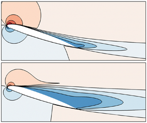
The streamwise velocity of steady solutions, corresponding to angles of attack marked with black dots in figures 1(a) and 1(b), is displayed in figure 1(c–g). For low angles of attack the flow is mostly attached, as seen in figure 1(c) for  $\alpha = 16.00^\circ$, which corresponds to the end of the linear increase in lift. Flow separation occurs very close to the trailing edge of the airfoil. On the other hand, for high angles of attack, the flow is mostly separated, as seen in figure 1(g) for
  $\alpha = 22.00^\circ$. The flow separates close to the leading edge of the airfoil and two recirculation regions, corresponding to negative streamwise velocity, exist in the wake of the airfoil. For intermediate values displayed in figure 1(d–f), the separation point continuously moves towards the leading edge when increasing the angle of attack and decreasing the lift. This is a characteristic feature of a trailing-edge stall mechanism (McCullough & Gault Reference McCullough and Gault1951). These pictures also illustrate the different base flows obtained for the same angle of attack
  $\alpha =18.45^\circ$ but corresponding to the upper, middle and lower branches of steady solutions.
3.2. High-frequency vortex-shedding and low-frequency stall modes
The linear stability of these steady branches is investigated, revealing two types of mode, which become unstable at different angles of attack. Figure 2(a) displays the eigenvalue spectra obtained close to the stall angle ( $\alpha =18.49^\circ$, triangles) and for larger angle of attack (
 $\alpha =22.00^\circ$, circles).

Figure 2. Characteristics of the unstable modes for two particular steady solutions. (a) Spectra represented in the complex plane  $(\sigma ;\omega )$. Triangles correspond to the spectrum obtained for
  $\alpha = 18.49^\circ$ on the upper branch and circles correspond to the spectrum obtained for
  $\alpha = 22.00^\circ$. The unstable eigenvalues are depicted in red. (b,c) Structure of the unstable eigenmodes
  $\hat {\boldsymbol {q}}(\alpha )$ represented by the streamwise velocity component
  $\hat {\rho u}$. The solid black line indicates the isocontour of zero-velocity of the mean flow in order to locate the recirculation zone. (b) Here
  $\alpha = 18.49^\circ$ on the upper branch (corresponding to the red triangle). (c) Structure of the unstable eigenvalue for
  $\alpha = 22.00^\circ$ on the lower branch (corresponding to the red circle).
At high angles of attack, when the base flow is fully separated, a high-frequency eigenvalue is unstable. The corresponding spatial structure, whose real component is displayed in figure 2(c), reaches its largest amplitude downstream of the recirculation region and slowly decreases in the far field wake. The two rows of streamwise oscillating structures that are out of phase in the cross-stream direction are typical of vortex-shedding modes, as described in many papers such as Marquet et al. (Reference Marquet, Sipp, Chomaz and Jacquin2008) in the case of a cylinder at Reynolds number  $Re = 46.8$. Superimposed onto the steady flow, they generate structures that are alternately shed from the recirculation bubble, a typical feature of bluff body unsteadiness (Roshko Reference Roshko1954). The angular frequency of
  $\omega = 0.573$ corresponds to a Strouhal number based on the projected surface (defined as
  $St = \omega c \sin (\alpha ) /(2{\rm \pi} U_\infty )$) of
  $St = 0.213$, which is in good agreement with
  $St \approx 0.2$ commonly accepted for this phenomenon.
Around the stall angle, a low-frequency eigenvalue is unstable (red triangles in figure 2a). The angular frequency is  $\omega = 0.0086$ , which corresponds to a Strouhal number of
  $St = 0.00271$, two orders of magnitude lower than the vortex-shedding Strouhal number. The spatial structure of the corresponding mode is displayed in figure 2(b) by its real part. It is elongated in the streamwise direction, with largest magnitude close to the separation point of the base flow and in the shear layer of the recirculation region. This is in good agreement with the mode identified by Iorio et al. (Reference Iorio, Gonzalez and Martinez-Cava2016) on an NACA
 $0012$ at very high Reynolds number,
  $Re = 6.0 \times 10^6$. Superimposed onto the base flow, it modifies the location of the separation point and the size of the recirculation region. This recirculation region slowly oscillates from a small trailing edge bubble to a large recirculation region extending over a large part of the suction side of the airfoil. In other words, it makes the flow switch between the attached and fully separated states. The characteristics of the so-called stall mode strongly echo the characteristics of these low-frequency oscillations (known as LFO) described, for instance, by Zaman, McKinzie & Rumsey (Reference Zaman, McKinzie and Rumsey1989).
The stall and vortex-shedding mode are not simultaneously unstable for the case studied here. Their domains of instability are indicated in figure 1(a) with dashed lines. The stall mode is unstable close to the stall angle (see figure 1b) when the lift suddenly drops, while the vortex-shedding mode becomes unstable at larger angle of attack  $\alpha >20.5^\circ$, when the base flow is massively separated.
For the remainder of the paper, we analyse the stall mode further (figure 2b) by tracking it along the three branches of steady solutions shown in figure 1(b). While its spatial structure is very similar for all angles of attack close to the stall angle, the evolution of the eigenvalue reveals several bifurcations. The location of the eigenvalue in the  $(\sigma , \omega )$ plane along the polar curve is presented in figure 3. On the major part of the upper branch, labelled
  $1$ in figure 3(a), the stall mode is stable and oscillatory (a pair of complex conjugate eigenvalues) as illustrated in figure 3(b). In this part of the curve, as the curvilinear abscissa (here the angle) increases, the stall mode becomes less damped and its angular frequency decreases. At the point on the upper branch labelled
  $H_U$ in figure 3(a), there is a Hopf bifurcation, i.e. the stall mode becomes marginally stable (see figure 3c). For larger angles of attack, the stall mode becomes unstable and its frequency continues to decrease (state
  $2$ and figure 3d) until, at the point labelled
  $D_U$, it reaches the axis
  $\omega =0$. This state, which is illustrated in figure 3(e) and is known as two-fold degenerate, is characterized by two identical positive real eigenvalues corresponding to different eigenmodes. By further increasing the curvilinear abscissa, the two identical real eigenvalues separate (state
  $3$ and figure 3f), one becoming less unstable and the other more unstable. When the least unstable real eigenvalue becomes marginally stable there is a saddle-node bifurcation (state
  $SN_U$ and figure 3g). This corresponds to the end of the upper branch and the beginning of the middle branch, labelled
  $4$ in figure 3(a). The whole middle branch is characterized by one stable real eigenvalue and one unstable real eigenvalue (figure 3h). Starting from
  $SN_U$ and moving along the polar curve by decreasing the angle of attack, the two real eigenvalues move away until at some point in the middle of the branch, they start to move closer. By doing so, the stable real eigenvalue becomes marginally stable again at the other extremity of the middle branch, labelled
  $SN_L$ in figure 3(a). Finally, when further increasing the angle of attack, the same succession of states and bifurcations is observed on the lower branch, but in a reversed order compared with the upper branch.

Figure 3. Evolution of the stall (low-frequency) eigenvalue along the branches of steady solutions. (a) Lift coefficient as a function of the angle of attack, with the stable and unstable branches indicated by solid and dashed curves, respectively. Eigenvalue spectra, corresponding to the four instability states indicated by numbers  $1$ to
  $4$, are sketched in panels (b), (d), (f) and (h). Sketches in panels (c), (e) and (g) correspond to the Hopf bifurcations (
 $H_{U/L}$), the two-fold degenerate eigenvalue (
 $D_{U/L}$) and the saddle-node bifurcations (
 $SN_{U/L}$), respectively, with the subscript
  $u$ and
  $l$ referring to the upper and lower branches. The colours indicate the type of unstable eigenvalues: blue for a pair of complex conjugate, red for two real unstable and green for one stable/one unstable real eigenvalues.
The exact positions of the bifurcation points are given in table 1. Note that the growth rate of the two identical eigenvalues is larger on the lower branch ( $D_L$) than on the upper branch (
 $D_U$). This results in the angular frequency being two times larger for the Hopf bifurcation on the lower branch (
 $H_L$) than on the upper branch (
 $H_U$). Also, as a consequence, the domain labelled
  $2$ in figure 3(a) is wider on the lower branch than on the upper branch (
 ${\rm \Delta} C_L \approx 6.81 \times 10^{-2}$ and
  ${\rm \Delta} C_L \approx 5.2 \times 10^{-3}$, respectively).
Table 1. Positions of the steady solutions in the  $(\alpha ;C_L)$ plane and of the associated eigenvalues in the complex plane
  $(\sigma ;\omega )$ for the bifurcations
  $H, SN$ and
  $D$ on the upper and lower branches introduced in figure 3 (subscripts
  $U$ and
  $L$, respectively).

3.3. Nonlinear low-frequency flow oscillations around stall
The destabilization of a low-frequency stall mode on the high- and low-lift steady branches suggests the existence of nonlinear low-frequency limit-cycle solutions. In the following, they are first investigated based on unsteady RANS computations. Secondly, to better understand their appearance and disappearance, a nonlinear one-equation static stall model is proposed to determine the unstable limit-cycle solutions, thus completing the bifurcation diagram.
Let us first consider the angle of attack  $\alpha = 18.49^\circ$ for which the steady solution on the lower (respectively, upper/middle) branch is stable (respectively, unstable) as seen in figure 1(a). Using the steady solution of the unstable upper branch as an initial condition of a time-resolved RANS computation, the large-amplitude limit cycle shown in figure 4 is obtained. As seen from the temporal evolution of the lift coefficient (the red curve in figure 4a), this limit cycle is characterized by a low-frequency and large-amplitude lift oscillation. The low angular frequency
  $\omega = 0.0132$ oscillation, which corresponds to Strouhal number
  $St = 0.00416$, is in reasonable agreement with the angular frequency of the stall eigenmode at this angle:
  $\omega = 0.0086$ and
  $St = 0.00271$. Interestingly, the limit cycle exceeds the amplitude of the high-lift and low-lift steady branches, both displayed with black horizontal dashed and solid lines, respectively, in figure 4(a). When the lift coefficient reaches its highest value, the flow is mostly attached to the airfoil and is only separated at the rear part of the profile, as seen in figure 4(b). As the separation moves upstream in figure 4(c) the lift decreases, and when it reaches its minimal value the flow is nearly fully separated (figure 4d). The minimal value of the unsteady lift is significantly lower than the steady lift of the lower branch. During the second half-period of the limit cycle (not shown here), the separation point moves downstream and the lift increases. The oscillation of the lift is thus clearly associated with an oscillation between mostly attached and nearly fully separated flows. These unsteady flow states (figures 4b and 4d) compare well with the steady flow states obtained on the upper and lower branches of solutions (figures 1d and 1f), due to the low value of the oscillation frequency. However, the maximum and minimum values of the unsteady lift are larger and smaller, respectively, than the steady values. Any time-resolved RANS computation initialized with an unstable steady solution on the upper branch (upper dashed blue line in figure 3a) converges to a low-frequency limit cycle. On the contrary, initializing time-resolved computations with any steady solution of the lower branch (bottom dashed blue line in figure 3a) converges to the high-lift steady solution. This is illustrated in figures 5(a) and 5(b), which display the temporal evolution of the lift coefficient for different initial conditions and two angles of attack,
  $\alpha = 18.42^\circ$ and
  $\alpha = 18.48^\circ$, respectively. For
  $\alpha = 18.42^\circ$, the steady solutions on the middle and lower branches are unstable and evolve (red and black curves) towards the high-lift steady solution, which is stable (blue curve). For
  $\alpha = 18.48^\circ$, only the middle-lift steady solution is unstable, and it converges, again, towards the high-lift steady solution, as shown in figure 5(b).

Figure 4. Solutions of the time-resolved RANS equations obtained for  $\alpha = 18.49^\circ$. (a) Temporal evolution of the lift coefficient exhibiting a low-frequency
  $\omega =0.014$ periodic behaviour. The horizontal dashed lines indicate the lift coefficients of the steady solutions for the steady lower and middle branches, which are linearly unstable, and the horizontal solid line indicates the lift coefficient of the steady lower branch, which is linearly stable. The initial condition of the unsteady simulation is the steady upper solution. (b–d) Instantaneous streamwise momentum
  $\rho u$ at three instants over half a period indicated with dots in panel (a).

Figure 5. Temporal evolution of the lift coefficient obtained for different initial flow states for (a)  $\alpha = 18.42^\circ$ (b) and
  $\alpha = 18.48^\circ$. Blue, red and black curves correspond to slightly perturbed upper, middle and lower steady solutions as initial flow states, respectively.
To assess the existence of the limit cycle for all angles of attack, a simple continuation method is used starting from the periodic solution at  $\alpha =18.49^\circ$. Time-resolved computations are successively performed by progressively decreasing (or increasing) the angle of attack using as an initial condition a snapshot of the limit cycle computed for the previous larger (respectively, smaller) values of the angle. Results are shown in figure 6(a) by depicting in red the mean and extrema values of the limit cycles as a function of the angles of attack, superimposed onto the steady solutions shown in black. The Strouhal number of these limit cycles is displayed in figure 6(b). The low-frequency limit cycles exist in a small range of angles of attack
  $18.464^\circ \le \alpha \le 18.510^\circ$. The time-averaged, minimal and maximal values of the lift vary slightly with the angle. In particular, the peak-to-peak amplitude of the limit cycle is very large, very close to the minimal (
 $\alpha =18.464^\circ$) and maximal (
 $\alpha =18.510^\circ$) angles, indicating an abrupt disappearance of the limit cycle for slightly lower or higher angles.

Figure 6. (a) Lift coefficient of the steady (black) and unsteady (red) solutions as a function of the angle of attack  $\alpha$. Stable and unstable steady solutions are depicted with solid and dashed black curves, respectively, while the time-averaged and peak-to-peak amplitude of the unsteady solutions are displayed with bullets and range bars, respectively. (b) Strouhal number of the periodic solutions as a function of
  $\alpha$. The vertical dashed lines indicate the minimal and maximal angles for which the periodic solution ceases to exit (in the grey regions, the time-resolved computations converge towards steady solutions).
Interestingly, the minimal and maximal angles for the existence of a limit cycle do not correspond to those of the critical angles  $\alpha _{H_{U}}=18.487^\circ$ (respectively,
  $\alpha _{H_{L}}=18.453^\circ$) associated with the upper and lower Hopf bifurcations, suggesting that these Hopf bifurcations are subcritical. These local bifurcations, which will be discussed again later using a nonlinear reduced-order stall model, therefore do not explain the onset and disappearance of the large-amplitude limit cycles close to the minimal and maximal angles. This phenomenon is actually related to a global bifurcation. We observe in figure 6(b) that the oscillation frequency rapidly decreases when approaching the minimal angle. This behaviour is characteristic of a homoclinic bifurcation, which corresponds to the collision of a periodic orbit with a saddle-node point in phase space (the system stays close to the saddle-node point for increasingly long times, which explains why the period of the limit cycle increases). To illustrate this collision better, we display in figure 7(a–c) the low-frequency periodic solutions for three angles of attack around the minimal angle in the
  $(\mathrm {d}{C_L}/\mathrm {d}t, C_L)$ plane. The large-amplitude periodic solution revolves around the three steady solutions marked with bullets (black for stable, white for unstable). When decreasing the angle of attack from
  $\alpha =18.47^\circ$ (figure 7c) to
  $\alpha =18.464^\circ$ (figure 7b), the periodic orbit shrinks in the
  $\mathrm {d}{C_L}/\mathrm {d}t$ direction and approaches the unstable middle steady solution, which is an unstable saddle-node in phase space (the middle steady solution has one unstable eigenvalue and one stable one by definition). Then, by slightly decreasing the angle of attack to
  $\alpha =18.4637^\circ$ (figure 7a), the limit cycle disappears and the unsteady orbit converges towards the high-lift steady solution.

Figure 7. Periodic orbits (curves), steady stable (black circles) and unstable (white circle) solutions displayed in the plane  $(\dot {C_L};C_L)$ for increasing values of the angles of attack close to (a–c) the minimal angle and (d–f) the maximal angle for the existence of limit cycles. The exact values of the angle are (a)
  $\alpha = 18.4637^\circ$ (just below the minimal angle of existence of limit cycle, explaining why the trajectory converges to the upper steady solution), (b)
  $\alpha = 18.464^\circ$ (minimal angle), (c)
  $\alpha = 18.47^\circ$, (d)
  $\alpha = 18.49^\circ$, (e)
  $\alpha = 18.51^\circ$ (maximal angle) and (f)
  $\alpha = 18.515^\circ$ (just above the maximal angle of existence of the limit cycle, explaining why the trajectory converges to the lower steady solution).
We now focus on the disappearance of the low-frequency flow oscillation when the angle of attack is increased. We display in figure 7(d–f) similar phase diagrams for three angles of attack around the maximal value. For  $\alpha =18.49^\circ$ (figure 7d), the periodic orbit still oscillates around the three steady solutions. The unstable high-lift solution (top white circle) is very close to the unstable middle solution (bottom white circle), meaning that they both disappear when the angle is increased to
  $\alpha =18.51^\circ$ (figure 7e) due to the saddle-node bifurcation previously described in § 3.2, which occurs at
  $\alpha =18.49203$ (see table 1). The periodic orbit has a large amplitude and reaches large lift values, which are typical of the upper steady branch that has disappeared. This limit cycle finally disappears as the angle is increased further, with the orbit spiralling down towards the lower-lift solution, as seen in figure 7(f).
Close to the maximal angle there is no sign of a homoclinic bifurcation, since neither the amplitude nor the frequency of the limit cycle suddenly decrease. It is worth recalling here that this limit cycle exists for angles at which the low-lift steady solution is stable, strongly indicating that the lower Hopf bifurcation  $H_L$ is subcritical. Such a bifurcation is difficult to identify by integrating the unsteady RANS equations in time, mainly because the unstable periodic solutions emerging from the Hopf bifurcation cannot be computed with a time stepper.
To confirm the nature of this bifurcation, we introduce the following low-order model that governs the time-evolution of the lift coefficient  $C_L$:
 \begin{equation} \frac{\textrm{d}^2 C_L}{\textrm{d} t^2} + P(C_L - C_{L_S}) \frac{\textrm{d} C_L}{\textrm{d} t} + K \cdot (\alpha - \alpha_s + Q(C_L - C_{L_S} )) = 0 . \end{equation}
This is a nonlinear damped harmonic oscillator in which  $P$ and
  $Q$ are two polynomials of third and fourth order, respectively, (
 $P(C_L - C_{L_S})= \sum _{i=0}^{3} P_i(C_L-C_{L_S})^i$ and
  $Q(C_L - C_{L_S})=\sum _{i=1}^{4} Q_i(C_L-C_{L_S})^i$) and
  $K, C_{L_S}$ and
  $\alpha _S$ are real constants. The angle of attack
  $\alpha$ is a parameter of the model. The pair
  $(\alpha _S, C_{L_S})$ is the coordinate of one particular point of the steady solutions curve, which is defined by the user. The coefficients of the polynomial
  $Q$ are calibrated using four points of the steady lift polar curve computed with the RANS equations. The coefficients of the polynomial
  $P$ and the constant
  $K$ are calibrated by using two objective functions. These functions are defined by minimizing the sum of the quadratic errors between the stall mode's growth rate (respectively, angular frequency) obtained with the linear stability analysis and obtained with the stall model for each steady solution of the polar curve. Therefore, all the eigenvalues computed between
  $18.35^\circ < \alpha < 18.50^\circ$ are used in the calibration process. The NSGA-II algorithm (Deb & Agarwal Reference Deb and Agarwal1995; Deb et al. Reference Deb, Pratap, Agarwal and Meyarivan2002) is used to solve this multi-objective problem. The calibration process is further detailed in Busquet (Reference Busquet2020). The results of the calibration are given in table 2. Generally speaking, the polynomial
  $Q(C_L)$ allows us to capture the three branches of steady lift while the polynomial
  $P(C_L)$ and coefficient
  $K$ allow us to recover the unstable behaviour of these branches.
Table 2. Calibrated values of the coefficients of the one-equation stall model (3.1). Here  $P_i$ and
  $Q_i$ are the coefficients of the polynomials
  $P$ and
  $Q$.
$Q$.

Once the model has been calibrated, its dynamical behaviour is investigated by using MatCont (Dhooge et al. Reference Dhooge, Govaerts, Kuznetsov, Meijer and Sautois2008), a MATLAB code for the study of dynamical systems. The steady and time-periodic solutions of the one equation stall model are, respectively, shown with black and red colours in figure 8. We observe a fairly good agreement between the steady solutions (black curves) of the low-order model and those of the (U)RANS model (see figure 6a), which validates the calibration process. The limit cycles are represented by their mean values (red squares) and peak-to-peak values (red range bars): filled squares for stable limit cycles and empty squares for unstable ones. We observe that the large amplitude stable limit cycles surrounding the three steady solutions are well captured, although their range is slightly shifted towards higher  $\alpha$ values. The results of the one-equation model provides an explanation for the disappearance of the limit cycle at the maximal angle of attack. First, these results show that the Hopf bifurcation
  $H_L$ on the lower steady branch is subcritical: the peak-to-peak amplitude of the emerging unstable limit cycle (range bars associated with empty squares) grows along the low-lift unstable branch for increasing angles of attack. For
  $\alpha =18.4993^\circ$, the unstable limit cycle collides with the large-amplitude cycle, as depicted in figure 8(a), and both disappear for larger angles. This is by definition a saddle-node bifurcation of periodic orbits, which is thus responsible for the disappearance of the low-frequency flow oscillations around the maximal angle of attack.

Figure 8. (a) Steady (black) and periodic (red) solutions of the one-equation model shown in in the  $C_L$–
 $\alpha$ diagram. Periodic solutions obtained with the URANS computations are depicted in grey for comparison. (b) Close-up view around the Hopf and saddle node bifurcation on the branch of high-lift steady solutions. Solid and dashed curves represent stable and unstable steady solutions, respectively. The mean values of the stable and unstable periodic solutions, emerging from the Hopf bifurcation point
  $H_U$ and
  $H_L$, are depicted with filled and empty squares, respectively. The range bars show the peak-to-peak amplitudes. To ease the reading of this figure, the limit cycle growing from the upper (respectively, lower) Hopf bifurcation is intentionally not represented in panel (a) (respectively, b).
Interestingly, the stall model shows that the upper Hopf bifurcation  $H_U$ is also subcritical. The unstable limit cycle which emerges from that bifurcation point is visible in figure 8(b), where we observe that, when decreasing the angle, the amplitude of this limit cycle slightly grows before suddenly disappearing. This is a second homoclinic bifurcation, which is clearly visible in this lift diagram. Indeed, the unstable small-amplitude limit cycle (range bar associated with empty squares) collides with the steady solution of the middle branch (back dashed curve) at
  $\alpha =18.4904^\circ$, when reaching its minimal lift value during the periodic motion. This homoclinic bifurcation should not be confused with the homoclinic bifurcation explaining the disappearance of the stable large-amplitude limit cycle. The collision for the latter with the steady solution of the middle branch is not visible in this lift diagram because it does not occur when the limit cycle reaches its minimal or maximal lift (see figure 7b). Note that the bifurcation scenario remains the same when modifying each parameter one-by-one by
  $1\,\%$ of their value. The present results compare well with those of numerical studies found in the literature. The hysteresis extends over a range of angle
  ${\rm \Delta} \alpha \sim 0.1^\circ$, which is in good agreement with the range of
  ${\rm \Delta} \alpha \sim 0.06^\circ$ identified by Richez et al. (Reference Richez, Leguille and Marquet2016) on the same airfoil in the same flow configuration. Moreover, the middle branch of steady solution, linking the branches of high and low lift solutions, is similar to the one identified by Wales et al. (Reference Wales, Gaitonde, Jones, Avitabile and Champneys2012) for an NACA
 $0012$ airfoil at
  $Re = 1.85 \times 10^6$. Finally, the linear stability analysis reveals the destabilization of an eigenmode occurring when the lift coefficient drops. The structure of the mode and its Strouhal number compare reasonably well with the one identified by Iorio et al. (Reference Iorio, Gonzalez and Martinez-Cava2016) who studied an NACA
 $0012$ at Reynolds number
  $Re = 6.0 \times 10^6$. They also noted that a large amplitude low frequency limit cycle emerges from this unstable mode. Interestingly, they obtained this low-frequency limit cycle without noticing any flow hysteresis. This strongly suggests that the destabilization of the stall mode and the resulting limit cycle are not dependent on the existence of a hysteresis of steady solutions. In the next section, we further explore that statement by investigating the flow around the same airfoil but at a lower value of the Reynolds number.
3.4. Bifurcation scenario for  $Re=5\times 10^5$

A similar investigation is now performed for the lower Reynolds number  $Re = 5.0 \times 10^5$, for which steady solutions do not exhibit hysteresis, as illustrated in the polar curve in figure 9(a). The steady solution is stable (black solid curve) for all angles of attack except in a small range
  $16.88^\circ \leq \alpha \leq 17.01^\circ$ (black dashed curve) where low-frequency eigenmodes are unstable. Low-frequency periodic solutions, with a Strouhal number in the range
  $0.005\leq St \leq 0.006$, exist for several angles of attack as illustrated in figure 9(a) in which limit cycles are represented by their mean values (red squares) and variations of lift coefficient (red range bars). The evolution of the eigenvalues as a function of
  $\alpha$ has several similarities with the bifurcation scenario previously described in figure 3(b–d) (the same numbering and letters have been used). In the prestall configuration, an oscillatory stable mode is identified. As the angle of attack increases, the oscillatory mode becomes unstable and its frequency decreases. By further increasing the angle of attack, this mode becomes stable again and its frequency increases. The main difference between the two scenarios comes from the fact that the stall mode never becomes steady, preventing the appearance of a saddle-node bifurcation. Moreover, the existence of limit cycles for angles of attack at which the steady solutions are stable indicates that the Hopf bifurcations are subcritical, which seems to be coherent with the results of the previous case. One can observe in figure 9(b–d), which present the evolution of the limit cycle for different angles of attack in the
  $(\mathrm {d}{C_L}/\mathrm {d}t,C_L)$ plane, that the periodic orbit never seems to move towards a steady solution, indicating that there is no homoclinic bifurcation involved in this scenario. Instead, extrapolating the results from the previous cases, it seems that the disappearance of the limit cycle is due on both ends to saddle-node bifurcations of periodic orbits. These assumptions have been confirmed with a newly calibrated one-equation stall model.

Figure 9. Low-frequency flow oscillation without hysteresis around the OA $209$ airfoil at
  $Re = 5 \times 10^5$. (a) Polar curve representing stable steady solutions (solid black lines), unstable steady solutions (dashed black lines) and periodic solutions characterized by their mean values (red squares) and peak-to-peak values (red range bars). (b–d) Limit cycles represented in the
  $(\dot {C_L};C_L)$ plane (phase diagrams) for different increasing angles of attack: (b)
  $\alpha = 16.87^\circ$, (c)
  $\alpha = 16.93^\circ$ and (d)
  $\alpha = 17.02^\circ$. The solid and open circles represent the stable and unstable steady solutions, respectively.
This results can be discussed in light of those obtained by Iorio et al. (Reference Iorio, Gonzalez and Martinez-Cava2016) for an NACA $0012$ profile. More specifically, they tracked the evolution of the stall mode/eigenvalue computed for the upper-lift steady solution and observed the following behaviour, similar to our results. In the prestall configuration, as the angle of attack is increased, the eigenmode becomes less stable and, simultaneously, its angular frequency decreases. Subsequently, the eigenmode becomes unstable and its angular frequency continues to decrease until the most unstable eigenmode is reached. Note that they did not track the eigenmode further as they did not compute the branch of unstable steady solutions. Nevertheless, based on what we observed on the OA
 $209$ airfoil at
  $Re = 5 \times 10^5$, it is likely that the mode would have stabilized again and its angular frequency would have increased at larger angles of attack.
3.5. Discussion
The results of our numerical study are now discussed by first exemplifying the similarities with numerical or experimental results previously published, and then discussing the discrepancies for the specific OA $209$ airfoil investigated here.
The unsteady low-frequency/large-amplitude limit cycle captured here with the fully turbulent URANS model has many features in common with low frequency oscillations described in various experimental and numerical studies (Zaman et al. Reference Zaman, Bar-Sever and Mangalam1987; Bragg & Zaman Reference Bragg and Zaman1994; Broeren & Bragg Reference Broeren and Bragg1998; Almutairi & AlQadi Reference Almutairi and AlQadi2013; Hristov & Ansell Reference Hristov and Ansell2018; ElJack & Soria Reference ElJack and Soria2018). By experimentally studying several airfoils at several Reynolds numbers, Broeren & Bragg (Reference Broeren and Bragg1998) established a correlation between the stall type and the characteristics of the low-frequency flow oscillation. They showed that the latter occurs for airfoils exhibiting trailing edge stall but not for leading edge stall. The largest variations in lift coefficient are obtained for those exhibiting a combined thin airfoil/trailing edge stall. In such cases, the maximum variations of lift coefficient observed are  $C_{L_{rms}} \approx 0.2$. In the present numerical study, we indeed obtain a trailing edge stall and observe the low-frequency oscillation. The variations of the lift
  $C_{L_{rms}} \approx 0.14$ compare relatively well, even though our configuration exhibits only trailing edge stall. The Strouhal number of this phenomenon for the OA
 $209$ (
 $St \sim 0.004$ for both Reynolds number explored here) is close to the values reported by Ansell & Bragg (Reference Ansell and Bragg2016) that lie in the range
  $0.005 < St < 0.03$ (for several smooth airfoils) with a tendency to increase as the stall angle increases. Secondly, the lift coefficient variations are caused by successive switching of the flow between stalled and unstalled states. They are attributed in the literature to a combination of two phenomena: a displacement of the trailing-edge separation point towards the leading edge and a laminar separation bubble whose reattachment point moves toward the trailing edge. When the two points collide, a massive flow separation is identified (Broeren & Bragg Reference Broeren and Bragg2001). In the present study, we also identify this switch between stalled and unstalled states, but it is only due to the motion of the trailing-edge separation, since our fully turbulent model does not allow us to capture the laminar separation bubble at the leading edge.
We now provide a more quantitative comparison of our results obtained for the OA $209$ airfoil at
  $\textit {Re}=1.8 \times 10^6$ with the experimental results obtained by Pailhas et al. (Reference Pailhas, Houdeville, Barricau, Le Pape, Faubert, Loiret and David2005) and the numerical results obtained by Richez et al. (Reference Richez, Leguille and Marquet2016) with the
  $k - \omega$ turbulence model. Figure 10 shows the lift coefficients as a function of the angle of attack for the three cases, which are notably different. According to the experimental data, displayed with square symbols, stall occurs abruptly around a
  $16^\circ$ angle of attack, suggesting that it is related to the bursting of a laminar separation bubble at the leading edge. The vertical bars, representing the amplitude variation, show that small-amplitude oscillations already occur in the prestall regime for
  $\alpha \sim 15^\circ$, while larger-amplitude oscillations occur in the poststall regime for
  $\alpha \ge 16$. These oscillation cycles are due to the vortex-shedding phenomenon and not to the low-frequency oscillation for which the amplitude variation is much larger. The latter may also exist but could not be confirmed with any of the measurements since it was not the objective of the experimental campaign reported in Pailhas et al. (Reference Pailhas, Houdeville, Barricau, Le Pape, Faubert, Loiret and David2005). Examining now the numerical results depicted with curves, they manifest a high sensitivity to the turbulence modelling. In particular, the stall is obtained at a higher angle of attack with the Spalart–Allmaras model (solid curve) than with the
  $k-\omega$ model (dashed curve). Both models have large discrepancies with the experimental data. This can be partially attributed to the inability of the fully turbulent RANS model to capture the laminar separation bubble around the leading edge. Indeed, for such high-Reynolds-number flows, the laminar separation bubble should occur very close to the leading edge so that the development of the turbulent boundary layer over the whole airfoil may be significantly different. In particular, it may also impact the location of the trailing-edge separation point, and thus the value of the aerodynamic coefficient. This clearly indicates that a transition model should be considered to obtain a more realistic and predictive description of the experimental observations. The methodology proposed in the present paper could then be used with this more sophisticated transition/turbulent RANS model. The discrepancies between numerical and experimental results can also be attributed to the simplified two-dimensional model used in the present paper. Indeed, three-dimensional stall cells may appear around the stall angle (Bertagnolio et al. Reference Bertagnolio, Sørensen and Rasmussen2005; Manni et al. Reference Manni, Nishino and Delafin2016; Plante et al. Reference Plante, Dandois and Laurendeau2020) and thus affect the aerodynamic coefficient. Interestingly, Plante et al. (Reference Plante, Dandois, Beneddine, Laurendeau and Sipp2021) recently showed that the onset of stall cells can be explained as the destabilization of three-dimensional steady global modes. Therefore, the present two-dimensional bifurcation scenario could be improved (and complexified) by taking into account the pitchfork bifurcation associated with stall cells.

Figure 10. Comparison of the evolution of the lift coefficient as a function of the angle of attack for the flow around an OA $209$ airfoil at
  ${Re = 1.8} \times 10^6$ from different studies: experimental study (Pailhas et al. Reference Pailhas, Houdeville, Barricau, Le Pape, Faubert, Loiret and David2005) (square symbols); two-dimensional numerical study with the
  $k-\omega$ turbulence model (Richez et al. Reference Richez, Leguille and Marquet2016) (dashed line); and the present study on a two-dimensional airfoil with the Spalart–Allmaras model (solid line). The vertical bars indicate the minimal and maximal values of lift oscillations observed experimentally or with URANS simulations when available.
To finish, we compare our results with the experimental results of Hristov & Ansell (Reference Hristov and Ansell2018), who investigated the stall of an NACA $0012$ airfoil at
  $Re = 1.0 \times 10^6$. To the authors’ knowledge, this is the only study reporting simultaneous hysteresis and low-frequency oscillations at such high Reynolds number, these phenomena being more often both observed at transitional Reynolds number
  $Re \sim \times 10^5$. The lift coefficient evolves relatively smoothly as is typical for trailing edge stall and they did not mention the existence of a laminar separation bubble. They also reported the existence of two branches of solutions in a range of angle of attack
  ${\rm \Delta} \alpha \sim 4^\circ$. These branches are characterized by two distinct unsteady phenomena: (i) a low-frequency unsteadiness, observed at the leading edge of the airfoil, which is characteristic of the high lift solutions at largest angle; and (ii) a high frequency unsteadiness, associated with vortex shedding, which is characteristic of the low lift solutions. This hysteresis of two unsteady solutions is, however, different from the hysteresis of steady solutions obtained in the present paper. It is worth noting that we have also captured the high-frequency unsteadiness with URANS simulations and global stability analysis, but for much larger angles of attack (
 $\alpha \ge 21.00^{\circ }$) than the stall angle. We speculate that, for different airfoils or other turbulence models, the vortex-shedding mode would be destabilized for angles close to the stall angle, and thus would modify the proposed bifurcation stall scenario.
4. Conclusion
In this paper we present the complete bifurcation diagram of a high-Reynolds-number flow around an OA $209$ airfoil. When modelled in the RANS framework, a trailing edge stall type is identified for this airfoil at high Reynolds number. Although this stall mechanism is not representative of a real flow, this configuration is used to propose new theoretical building blocks to describe trailing-edge stall exhibiting hysteresis and low-frequency oscillations. We start with the computation of steady solutions, revealing the inverted S-shaped polar curve characteristic of hysteresis in the flow. By conducting a linear stability analysis of all the steady solutions, we identify a mode that becomes unstable at stall. Along the polar curve this mode experiences several bifurcations: two Hopf bifurcations, two solutions with a two-fold degenerate eigenvalue, and two saddle-node bifurcations. The study of the unsteady nonlinear behaviour of the flow, with URANS computations and via a one-equation static stall model, reveals that these Hopf bifurcations are subcritical. The unstable limit cycle emerging from the lower Hopf bifurcation becomes stable in a saddle-node bifurcation of a periodic orbit. The resulting stable limit cycle strongly echoes low-frequency oscillations that are well documented in the literature with low Strouhal numbers, high amplitudes and similar flow behaviour. The disappearance of this limit cycle occurs when it collides with the middle branch of steady solutions in a homoclinic bifurcation. Finally, by comparing the two bifurcation scenarios investigated, one can conclude that: (i) stall occurs when the stall mode is unstable; (ii) hysteresis of the steady solution occurs when the stall mode becomes steady, leading to a saddle-node bifurcation; (iii) low-frequency oscillation is driven by the existence of the stall mode but is not related to the existence of hysteresis. In particular, the existence of low-frequency oscillation seems to be driven by the existence of subcritical Hopf bifurcations.
This study demonstrates the feasibility of establishing the bifurcation scenario of a high-Reynolds-number flow in the RANS framework, which, to the authors’ knowledge had not been achieved before. It also demonstrates that, despite the obvious limitations of the RANS modelling in predicting stall, this approach allows us to explain the appearance of hysteresis and low-frequency oscillations at high Reynolds number in the case of a trailing edge stall type, which is lacking in the literature.
These results raise further questions that should be investigated in the future. The first is how representative this scenario is of a real flow. The configuration studied by Hristov & Ansell (Reference Hristov and Ansell2018) is probably the most appropriate to compare with. Indeed, it seems to exhibit a stall mechanism close to the one identified in the present paper and in which hysteresis and low-frequency oscillations are known to exist over a wide range of angles of attack.
Finally, this study is a first step in combining bifurcation theory and RANS in order to study stall. Recent and forthcoming improvements in RANS modelling should allow better modelling of the flow behaviour at stall and, therefore, better prediction of hysteresis and stall angle with these techniques. These improvements might also, in the near future, offer the possibility of investigating bifurcation scenarios of flows around airfoils exhibiting different stall types and determine whether this bifurcation scenario applies to all airfoil or just to airfoil that exhibit trailing edge stall type.
Acknowledgements
The authors would like to thank S. Beneddine for his help and assistance on the linear stability analysis code. The authors are also grateful to L. Tuckerman for discussions about the bifurcation scenario.
Funding
This work was supported by a partnership between DGA and Dstl in the framework of a Franco–British collaboration.
Declaration of interests
The authors report no conflict of interest.
Appendix A. Description of the mesh
Figure 11 presents some features of the mesh used in this study: figure 11(a) is a visualization of the grid close to the airfoil and figure 11(b) provides the near wall grid resolution in the chordwise direction on the upper side of the airfoil. Particular attention has been paid to the grid refinement in the boundary layer of the suction side as well as in the wake. Also, an effort has been made to try to ensure as much as possible the local perpendicularity between the lines starting from the airfoil and the boundary C. This mesh is made of  $144\,352$ cells. The chordwise cell length is set to
  ${\rm \Delta} x/c =0.05\,\%$ at the leading edge and reaches
  ${\rm \Delta} x /c =0.55\,\%$ at midchord (solid line in figure 11b) which is close to the requirement provided by Costes et al. (Reference Costes, Richez, Le Pape and Gavériaux2015) for a similar airfoil in similar aerodynamic conditions. Expressed in wall units, the chordwise resolution ensures that
  ${\rm \Delta} x+ \leq 500$ at low angles of attack where the flow is fully attached (dashed line in figure 11b) and
  ${\rm \Delta} x^+ \leq 300$ close to stall angle of attack where the flow separation starts to appear on the suction side (dash–dotted line in figure 11b). In the wall normal direction, the grid resolution is fine enough to ensure
  ${\rm \Delta} y^+ <1$ at the wall and provides at least 40 points in the boundary layer at the leading edge and 70 points at midchord. This grid resolution is expected to minimize the effects of numerical dissipation on the flow solution.

Figure 11. Mesh resolution around the two-dimensional OA $209$ airfoil used in the present study. (a) Close-up view of the grid around the airfoil. (b) Near wall resolution in the chordwise direction on the upper side expressed in per cent of chord
  ${\rm \Delta} x /c$ (solid line) and in wall units
  ${\rm \Delta} x^{+}$ at
  $12^\circ$ (dashed line) and
  $16^\circ$ (dash–dotted line) angle of attack.
Appendix B. Computation of the Jacobian matrix by finite difference
In the present study, the choice is made to approximate the Jacobian matrix using a central finite difference method. The components of the matrix are computed as described by
 \begin{equation} J_{ij}(\boldsymbol{Q}_0,\alpha_{0}) = \left.\frac{\partial R_i}{\partial Q_j} \right|_{(\boldsymbol{Q}_0,\alpha_0)} = \frac{R_i(\boldsymbol{Q}_0+ \delta Q_j \boldsymbol{Q}^j,\alpha_0) - R_i (\boldsymbol{Q}_0 - \delta Q_j \boldsymbol{Q}^j,\alpha_0)}{2 \delta Q_j}, \end{equation}
where  $\delta Q_j$ is a small perturbation of the
  $j$th component of
  $\boldsymbol {Q}$ and
  $\boldsymbol {Q}^j$ is a vector for which the
  $j$th component of the vector is equal to one and null everywhere else. This method offers the advantage of being robust to changes of numerical methods, turbulence model or boundary conditions as any change is directly accounted for in the residual
  $\boldsymbol {R}$. The main drawback of the method is its sensitivity to the choice of the small perturbation
  $\delta Q_j$. This perturbation must be small enough to ensure the validity of the method (neglecting high-order terms in the Taylor expansion) but not too small to avoid rounding errors. In their study on Jacobian-free Newton–Krylov methods, Knoll & Keyes (Reference Knoll and Keyes2004) describe this choice ‘as much of an art as a science’. Mettot et al. (Reference Mettot, Renac and Sipp2014) suggested that
  $\delta Q_j$ should be chosen such that
  $\delta Q_j= \epsilon _m (|Q_j| + 1)$, with
  $Q_j$ the local value of the
  $j$th variable. The value of
  $\epsilon _m$ must be chosen with respect to machine precision and an optimal value is
  $\epsilon _m \approx 5 \times 10^{-6}$ in the case of a central finite difference (An, Wen & Feng Reference An, Wen and Feng2011). Mettot et al. (Reference Mettot, Renac and Sipp2014) considered this value and, additionally, noted that, in the case of the Spalart–Allmaras model, better results were obtained when considering a different value for the turbulent variable:
  $\epsilon _m / 10$. They observed that with such parameters, a convergence is obtained for
  $\epsilon _m < 10^{-5}$ in the case of a two-dimensional cavity. The same parameters are considered in the present study. In order to validate this choice, other values of
  $\epsilon _m$ are considered and the results are compared with the reference case
  $\epsilon _m = 5 \times 10^{-6}$. It was observed that values of
  $\epsilon _m = 10^{-5}$ and
  $\epsilon _m = 10^{-6}$ lead to errors of less than
  $0.5\,\%$ on the growth rate and the angular frequency of the stall mode.
Appendix C. Validation of the continuation methods
Figures 12(a) and 12(b) present the evolution of the global explicit residual of two variables ( $\rho$ and
  $\rho \tilde {\nu }$) in the case of the flow around an OA209 airfoil at
  $Re = 1.8 \times 10^6$ for
  $\alpha =12.20^\circ$ computed from a steady solution for
  $\alpha = 12.00^\circ$ with a Newton and a pseudo-arclength methods, respectively. These continuation methods require only a few iterations to converge (between
  $\sim 10^1$ and
  $\sim 10^2$) compared with the local time stepping approach. The residuals reach values of
  $\sim 10^{-12}$ for the conservative variable
  $\rho$ and
  $\sim 10^{-16}$ for the turbulent variable
  $\rho \tilde {\nu }$.

Figure 12. Evolution of the explicit residual for the conservative variable  $\rho$ (black curve) and the turbulent variable
  $\tilde {\nu }$ (red curve) for
  $\alpha = 12.20^\circ$ initialized with a solution for
  $\alpha = 12.00^\circ$. (a) Naïve continuation method and (b) pseudo-arclength method. Full diamonds correspond to the computation of the Jacobian matrix (and derivative vector if needed), associated factorization and inversion of the corresponding system. Full circles correspond to the inversion of the corresponding system only.
The difference of residual at the beginning of the iterative process is due to the solutions used as predictor, which are different in the two approaches. Moreover, one should be careful when comparing the convergence rates of the two methods. In the case of the naïve continuation method, the Jacobian was recomputed every five iterations (the corresponding steps are represented by diamonds in figure 12a) while in the case of the pseudo-arclength method, the Jacobian matrix and derivative vector were computed only at the beginning of the iterative process. This arbitrary choice was made because in the case of the naïve continuation method, we can afford to compute and factorize the Jacobian matrix as soon as the convergence rate seems to stagnate. However, in the case of the pseudo-arclength method, the non-sparsity of the assembled matrix requires more time to factorize and take more resource to store than performing  $50$ iterations. Note that specific tools could be implemented to facilitate this factorization and could improve the memory requirements as well as the computational time required to converge with the pseudo-arclength method.


