


1 Introduction
The Free Central Limit Theorem serves as a foundational principle in free probability [Reference Voiculescu16], [Reference Nica and Speicher12, Lecture 8]. It asserts that as the number of freely independent operators summed together approaches infinity, the distribution of the normalized sum tends toward an asymptotically semi-circular shape. This mirrors the classical Central Limit Theorem but with independence conditions replaced by free independence (also known as freeness) and the Gaussian limit substituted with a semi-circular limit. More precisely, let
 $(\mathcal {A},\tau )$
be a unital noncommutative probability space equipped with a faithful tracial state
$(\mathcal {A},\tau )$
be a unital noncommutative probability space equipped with a faithful tracial state
 $\tau $
[Reference Nica and Speicher12, Lecture 1]. We say that subalgebras
$\tau $
[Reference Nica and Speicher12, Lecture 1]. We say that subalgebras
 $\mathcal {A}_1,\ldots , \mathcal {A}_d\subset \mathcal {A}$
are free if
$\mathcal {A}_1,\ldots , \mathcal {A}_d\subset \mathcal {A}$
are free if
 $$ \begin{align*} \tau(a_1\ldots a_p)=0, \end{align*} $$
whenever
 $p \ge 1$
,
$p \ge 1$
,
 $a_i \in \mathcal {A}_{j_i}$
,
$a_i \in \mathcal {A}_{j_i}$
,
 $\tau (a_i)=0$
for all
$\tau (a_i)=0$
for all
 $i\in [p]$
and
$i\in [p]$
and
 $j_1 \ne j_2 \ne \ldots \ne j_p$
. We say that random variables
$j_1 \ne j_2 \ne \ldots \ne j_p$
. We say that random variables
 $a_1,\ldots ,a_d \in \mathcal {A}$
are free if their generated algebras are free. We denote
$a_1,\ldots ,a_d \in \mathcal {A}$
are free if their generated algebras are free. We denote
 $\mu _a$
the distribution of a (self-adjoint) random variable
$\mu _a$
the distribution of a (self-adjoint) random variable
 $a=a^*\in (\mathcal {A},\tau )$
, that is, the unique measure such that
$a=a^*\in (\mathcal {A},\tau )$
, that is, the unique measure such that
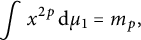
 $$ \begin{align*} \tau(a^p)=\int x^p\,\text{d}\mu, \end{align*} $$
for all integers
 $p\ge 1$
. We say that a sequence of (self-adjoint) variables
$p\ge 1$
. We say that a sequence of (self-adjoint) variables
 $a_n \in (\mathcal {A}_n,\tau _n)$
converges in distribution to a variable
$a_n \in (\mathcal {A}_n,\tau _n)$
converges in distribution to a variable
 $a \in (\mathcal {A},\tau )$
if
$a \in (\mathcal {A},\tau )$
if
 $$ \begin{align*} \tau_n(a_n^p) \to \tau(a^p), \end{align*} $$
for all integers
 $p \ge 0$
and we denote it
$p \ge 0$
and we denote it
 $a_n \Rightarrow a$
. Equivalently,
$a_n \Rightarrow a$
. Equivalently,
 $\mu _{a_n}$
converges weakly toward
$\mu _{a_n}$
converges weakly toward
 $\mu _a$
, and denoted by
$\mu _a$
, and denoted by
 $\mu _{a_n} \Rightarrow \mu _a$
. We denote
$\mu _{a_n} \Rightarrow \mu _a$
. We denote
 $a-\lambda :=a-\lambda \mathbf {1}$
, where
$a-\lambda :=a-\lambda \mathbf {1}$
, where
 $\mathbf {1} \in \mathcal {A}$
is the unit in the algebra. As usual,
$\mathbf {1} \in \mathcal {A}$
is the unit in the algebra. As usual,
 $\tau (a)$
is the mean of a and the variance is given by
$\tau (a)$
is the mean of a and the variance is given by
 $$ \begin{align*} \operatorname{var}(a)=\tau((a-\tau(a))^2). \end{align*} $$
The Free Central Limit Theorem states that if
 $a_1,\ldots ,a_n\in (\mathcal {A},\tau )$
are free self-adjoint identically distributed random variables with mean
$a_1,\ldots ,a_n\in (\mathcal {A},\tau )$
are free self-adjoint identically distributed random variables with mean
 $\lambda $
and variance
$\lambda $
and variance
 $\sigma ^2$
, then
$\sigma ^2$
, then
 $$ \begin{align*}\frac{1}{\sigma\sqrt{n}}\sum_{k\in[n]} (a_k-\lambda) \Rightarrow s, \end{align*} $$
where s is the standard semi-circle random variable, whose distribution
 $\mu _{sc}:=\mu _s$
has a density given by
$\mu _{sc}:=\mu _s$
has a density given by
 $$ \begin{align*} f_{sc}(x)=\frac{1}{2\pi}\sqrt{4-x^2} \mathbf{1}_{|x| \le 2}. \end{align*} $$
The goal of this paper is to establish a Central Limit Theorem for the tensor product of free random variables. Concretely, given
 $a_1,\ldots ,a_n\in (\mathcal {A},\tau )$
free self-adjoint identically distributed random variables, we aim at studying the convergence of the normalized sequence
$a_1,\ldots ,a_n\in (\mathcal {A},\tau )$
free self-adjoint identically distributed random variables, we aim at studying the convergence of the normalized sequence
 $$ \begin{align} \frac{1}{\sqrt{n}}\sum_{k \in [n]}\left(a_k \otimes a_k-\tau\otimes \tau(a_k\otimes a_k)\right)\hspace{-1.5pt}, \end{align} $$
in the product space
 $(\mathcal {A}\otimes \mathcal {A},\tau \otimes \tau )$
.
$(\mathcal {A}\otimes \mathcal {A},\tau \otimes \tau )$
.
Just as free probability captures the limiting behavior of random matrices, the above expression appears naturally as the limiting object corresponding to several models of random quantum channels [Reference Lancien, Santos and Youssef8]. Indeed, given
 $M_1,\ldots ,M_n \in \mathcal {M}_d(\mathbb {C})$
independent random self-adjoint matrices, it was shown in [Reference Lancien, Santos and Youssef8] that the empirical spectral distribution (ESD) of the quantum channel
$M_1,\ldots ,M_n \in \mathcal {M}_d(\mathbb {C})$
independent random self-adjoint matrices, it was shown in [Reference Lancien, Santos and Youssef8] that the empirical spectral distribution (ESD) of the quantum channel
 $$ \begin{align*} \Delta_{d,n}:=\frac{1}{\sqrt{n}}\sum_{k \in [n]} \left(M_k \otimes M_k-{\mathbb{E}} [M_k \otimes M_k]\right)\hspace{-1.5pt}, \end{align*} $$
having the
 $M_k$
’s as random Kraus operators and with fixed Kraus rank n, converges as
$M_k$
’s as random Kraus operators and with fixed Kraus rank n, converges as
 $d\to \infty $
to the expression in (1) with the
$d\to \infty $
to the expression in (1) with the
 $a_k$
’s being the corresponding limits of the ESD of the
$a_k$
’s being the corresponding limits of the ESD of the
 $M_k$
’s. Moreover, it was in particular shown that if the random matrices
$M_k$
’s. Moreover, it was in particular shown that if the random matrices
 $M_k$
are centered, then the ESD of
$M_k$
are centered, then the ESD of
 $\Delta _{d,n}$
converges as
$\Delta _{d,n}$
converges as
 $n,d\to \infty $
to the semi-circle distribution. These two statements combined suggest that, in the case where the
$n,d\to \infty $
to the semi-circle distribution. These two statements combined suggest that, in the case where the
 $a_k$
’s are centered, an analog of the Free Central Limit Theorem should hold for the
$a_k$
’s are centered, an analog of the Free Central Limit Theorem should hold for the
 $a_k\otimes a_k$
’s. Whereas these heuristics indicate that the semi-circle distribution should appear as the limit of (1) when the
$a_k\otimes a_k$
’s. Whereas these heuristics indicate that the semi-circle distribution should appear as the limit of (1) when the
 $a_k$
’s are centered, the convergence and the explicit limit are not clear in the general case. The goal of this paper is to address this by establishing the convergence of the expression in (1) and identifying the limiting object. The latter, as we show, depends on the mean and variance of the variables
$a_k$
’s are centered, the convergence and the explicit limit are not clear in the general case. The goal of this paper is to address this by establishing the convergence of the expression in (1) and identifying the limiting object. The latter, as we show, depends on the mean and variance of the variables
 $a_k$
’s and represents a free interpolation between a semi-circle distribution and the classical convolution of two semi-circle distributions.
$a_k$
’s and represents a free interpolation between a semi-circle distribution and the classical convolution of two semi-circle distributions.
Random matrix models of the form
 $$ \begin{align} M = \sum_{k \in [n]}M_k \otimes M_k, \end{align} $$
for
 $M_1,\ldots ,M_n \in \mathcal {M}_d(\mathbb {C})$
independent random self-adjoint matrices, are in fact useful in other areas of Quantum Information Theory. When the
$M_1,\ldots ,M_n \in \mathcal {M}_d(\mathbb {C})$
independent random self-adjoint matrices, are in fact useful in other areas of Quantum Information Theory. When the
 $M_k$
’s are positive semidefinite matrices, normalizing M by its trace produces a model for a random separable quantum state. Little is known about the typical asymptotic spectrum of separable states, contrary to that of entangled ones [Reference Ambainis, Harrow and Hastings1]. Moreover, a random matrix M of the form (2) appears naturally when performing a so-called realignment operation on a quantum state. Understanding the spectrum of the realignment of a state is important as it gives information on the entanglement of the state. In [Reference Aubrun and Nechita2], this was done in the particular case where the
$M_k$
’s are positive semidefinite matrices, normalizing M by its trace produces a model for a random separable quantum state. Little is known about the typical asymptotic spectrum of separable states, contrary to that of entangled ones [Reference Ambainis, Harrow and Hastings1]. Moreover, a random matrix M of the form (2) appears naturally when performing a so-called realignment operation on a quantum state. Understanding the spectrum of the realignment of a state is important as it gives information on the entanglement of the state. In [Reference Aubrun and Nechita2], this was done in the particular case where the
 $M_k$
’s are Gaussian matrices (corresponding to the case where the state is a normalized Wishart matrix). The results and techniques we develop here (combined with those in [Reference Lancien, Santos and Youssef8]) could be useful in addressing the questions mentioned above.
$M_k$
’s are Gaussian matrices (corresponding to the case where the state is a normalized Wishart matrix). The results and techniques we develop here (combined with those in [Reference Lancien, Santos and Youssef8]) could be useful in addressing the questions mentioned above.
Given a measure
 $\mu $
, we denote
$\mu $
, we denote
 $$ \begin{align*} (t\mu)(A):=\mu(t^{-1}A), \end{align*} $$
its dilation by
 $t \ne 0$
, where A is any Borel set in
$t \ne 0$
, where A is any Borel set in
 $\mathbb {R}$
. Equivalently, if a is a random variable with distribution
$\mathbb {R}$
. Equivalently, if a is a random variable with distribution
 $\mu $
, then
$\mu $
, then
 $ta$
has distribution
$ta$
has distribution
 $t\mu $
.
$t\mu $
.
The following is our main theorem.
Theorem 1.1 Let
 $a \in (\mathcal {A},\tau )$
be a self-adjoint random variable with mean
$a \in (\mathcal {A},\tau )$
be a self-adjoint random variable with mean
 $\tau (a)=\lambda $
and variance
$\tau (a)=\lambda $
and variance
 $\operatorname {var}(a)=\sigma ^2\ne 0$
. Denote
$\operatorname {var}(a)=\sigma ^2\ne 0$
. Denote
 $$ \begin{align*}\delta^2:=\operatorname{var}(a\otimes a)= \sigma^2(\sigma^2+2\lambda^2), \end{align*} $$
and
 $$ \begin{align*} q:=\frac{2\lambda^2}{\sigma^2+2\lambda^2} \in [0,1]. \end{align*} $$
Given
 $(a_k)_{k\in \mathbb {N}}$
a sequence of free copies of a, the distribution
$(a_k)_{k\in \mathbb {N}}$
a sequence of free copies of a, the distribution
 $\mu _{S_n}$
of the normalized sum
$\mu _{S_n}$
of the normalized sum
 $$ \begin{align*} S_n:= \frac{1}{\delta \sqrt{n}}\sum_{k \in [n]}(a_k\otimes a_k-\lambda^2) \end{align*} $$
converges weakly as
 $n\to \infty $
to
$n\to \infty $
to
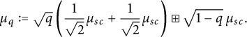
 $$ \begin{align} \mu_q:=\sqrt{q}\left(\frac{1}{\sqrt{2}}\mu_{sc}+\frac{1}{\sqrt{2}}\mu_{sc}\right)\boxplus\sqrt{1-q}\,\mu_{sc}, \end{align} $$
where
 $+$
denotes the classical convolution and
$+$
denotes the classical convolution and
 $\boxplus $
denotes the free convolution.
$\boxplus $
denotes the free convolution.
The difficulty in analyzing
 $S_n$
stems from the complicated dependence structure exhibited by tensors, combining classical independence (between the two legs of the tensor) and freeness (between the variables across tensors). In the centered case, similar computations were made for semi-circle random variables [Reference Dehornoy and Biane6, Reference Nica11]. It would be of interest to design a general notion of independence corresponding to the tensor case, analyze its properties, derive the corresponding limit theorems, and characterize the corresponding universal objects. One particular generalization is by replacing the tensor product with the product of
$S_n$
stems from the complicated dependence structure exhibited by tensors, combining classical independence (between the two legs of the tensor) and freeness (between the variables across tensors). In the centered case, similar computations were made for semi-circle random variables [Reference Dehornoy and Biane6, Reference Nica11]. It would be of interest to design a general notion of independence corresponding to the tensor case, analyze its properties, derive the corresponding limit theorems, and characterize the corresponding universal objects. One particular generalization is by replacing the tensor product with the product of
 $\varepsilon $
-independent random variables [Reference Młotkowski10, Reference Speicher and Weber14, Reference Speicher and Wysoczański15]. A direct consequence of Theorem 1.1 is that such a notion cannot, in general, reduce to freeness.
$\varepsilon $
-independent random variables [Reference Młotkowski10, Reference Speicher and Weber14, Reference Speicher and Wysoczański15]. A direct consequence of Theorem 1.1 is that such a notion cannot, in general, reduce to freeness.
Corollary 1.2 Let
 $a_1,\ldots ,a_n \in (\mathcal {A},\tau )$
be self-adjoint free identically distributed noncentered random variables. Then
$a_1,\ldots ,a_n \in (\mathcal {A},\tau )$
be self-adjoint free identically distributed noncentered random variables. Then
 $\{a_k\otimes a_k: k \in [n]\}$
are not free.
$\{a_k\otimes a_k: k \in [n]\}$
are not free.
The above corollary trivially follows from Theorem 1.1, since if the
 $a_k\otimes a_k$
’s were free, the limit of their normalized sum would be the semi-circle distribution contradicting the conclusion of Theorem 1.1 (when
$a_k\otimes a_k$
’s were free, the limit of their normalized sum would be the semi-circle distribution contradicting the conclusion of Theorem 1.1 (when
 $\lambda \neq 0$
). This fact was originally proved in [Reference Collins and Lamarre5] where, more generally, the freeness of tensors of free variables was characterized.
$\lambda \neq 0$
). This fact was originally proved in [Reference Collins and Lamarre5] where, more generally, the freeness of tensors of free variables was characterized.
We will provide two proofs of Theorem 1.1. The first proof relies on the computation of the limiting moments of
 $S_n$
and highlights the combinatorial structure of the set of partitions that have nonzero contributions. The second proof is shorter and explains the appearance of the three semi-circle random variables in the limiting law.
$S_n$
and highlights the combinatorial structure of the set of partitions that have nonzero contributions. The second proof is shorter and explains the appearance of the three semi-circle random variables in the limiting law.
This paper is organized as follows. In Section 2, we recall some definitions and notations. In Section 3, we provide some properties of the limiting measure appearing in Theorem 1.1. Section 4 establishes the existence of the limit, while Section 5 is dedicated to the proof of Theorem 1.1. Finally, in Section 6, we provide a short alternative proof of Theorem 1.1.
2 Preliminaries and notations
Given
 $p\in \mathbb {N}$
, a partition
$p\in \mathbb {N}$
, a partition
 $\pi =\{V_1, \ldots ,V_k\}$
of
$\pi =\{V_1, \ldots ,V_k\}$
of
 $[p]$
is a collection of nonempty disjoint sets
$[p]$
is a collection of nonempty disjoint sets
 $V_1,\ldots ,V_k$
called blocks such that
$V_1,\ldots ,V_k$
called blocks such that
 $$ \begin{align*} V_1 \cup \ldots \cup V_k=[p]. \end{align*} $$
We denote by
 $P(p)$
the set of partitions of
$P(p)$
the set of partitions of
 $[p]$
. We say that a partition
$[p]$
. We say that a partition
 $\pi \in P(p)$
is connected (also referred to as a linked diagram in [Reference Nijenhuis and Wilf13]) if no proper subinterval of
$\pi \in P(p)$
is connected (also referred to as a linked diagram in [Reference Nijenhuis and Wilf13]) if no proper subinterval of
 $[p]$
can be written as the union of blocks of
$[p]$
can be written as the union of blocks of
 $\pi $
. A partition
$\pi $
. A partition
 $\pi \in P(p)$
has a crossing
$\pi \in P(p)$
has a crossing
 $i<k<j<l$
if there exist two disjoint blocks
$i<k<j<l$
if there exist two disjoint blocks
 $V_1,V_2 \in \pi $
such that
$V_1,V_2 \in \pi $
such that
 $\{i,j\}\subset V_1$
and
$\{i,j\}\subset V_1$
and
 $\{k,l\} \subset V_2$
. In this case, we say that
$\{k,l\} \subset V_2$
. In this case, we say that
 $V_1$
crosses
$V_1$
crosses
 $V_2$
. A block
$V_2$
. A block
 $V\in \pi $
is crossing if there exists another
$V\in \pi $
is crossing if there exists another
 $V' \in \pi $
such that
$V' \in \pi $
such that
 $V'$
crosses V, and noncrossing if it does not cross any other block. We say that a partition
$V'$
crosses V, and noncrossing if it does not cross any other block. We say that a partition
 $\pi \in P(p)$
is a noncrossing partition if all its blocks are noncrossing. We denote by
$\pi \in P(p)$
is a noncrossing partition if all its blocks are noncrossing. We denote by
 $P^{\operatorname {con}}(p)$
(resp.
$P^{\operatorname {con}}(p)$
(resp.
 $NC(p)$
) the set of all connected (resp. noncrossing) partitions of
$NC(p)$
) the set of all connected (resp. noncrossing) partitions of
 $[p]$
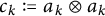
; see Figure 1. We note that the cardinal
$[p]$
; see Figure 1. We note that the cardinal
 $|NC(p)|$
is equal to
$|NC(p)|$
is equal to
 $C_p$
, the p-th Catalan number.
$C_p$
, the p-th Catalan number.

Figure 1: Examples of partitions.
Finally, for a partition
 $\pi \in P(p)$
, we denote by
$\pi \in P(p)$
, we denote by
 $G(\pi )$
its intersection graph. It is the graph over the blocks of
$G(\pi )$
its intersection graph. It is the graph over the blocks of
 $\pi $
such that two blocks are connected if they cross, under some arbitrary labeling. We say that a partition
$\pi $
such that two blocks are connected if they cross, under some arbitrary labeling. We say that a partition
 $\pi $
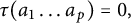
is a bipartite partition if its intersection graph is bipartite and denote it
$\pi $
is a bipartite partition if its intersection graph is bipartite and denote it
 $\pi \in P^{\operatorname {bi}}(p)$
; see Figure 2 for the partitions in Figure 1.
$\pi \in P^{\operatorname {bi}}(p)$
; see Figure 2 for the partitions in Figure 1.
Figure 2: Examples of intersection graphs.
Given
 $\pi \in P(p)$
, we denote
$\pi \in P(p)$
, we denote
 $|\pi |$
its number of blocks and
$|\pi |$
its number of blocks and
 $\mathbf {cr}(\pi )$
its number of crossing blocks. Therefore, the number of noncrossing blocks of
$\mathbf {cr}(\pi )$
its number of crossing blocks. Therefore, the number of noncrossing blocks of
 $\pi $
is
$\pi $
is
 $$ \begin{align*} \mathbf{ncr}(\pi):=|\pi|-\mathbf{cr}(\pi). \end{align*} $$
Given
 $\pi \in P(p)$
, we denote
$\pi \in P(p)$
, we denote
 $\mathbf {cc}(\pi )$
its number of connected components. We denote
$\mathbf {cc}(\pi )$
its number of connected components. We denote
 $P_2(p), P_2^{\operatorname {bi}}(p)$
,
$P_2(p), P_2^{\operatorname {bi}}(p)$
,
 $P_2^{\operatorname {con}}(p)$
,
$P_2^{\operatorname {con}}(p)$
,
 $P_2^{\operatorname {bicon}}(p)$
, and
$P_2^{\operatorname {bicon}}(p)$
, and
 $NC_2(p)$
the set of pair partitions, bipartite pair partitions, connected pair partitions, bipartite connected pair partitions, and noncrossing pair partitions, respectively, that is, those partitions such that all of their blocks have cardinality two.
$NC_2(p)$
the set of pair partitions, bipartite pair partitions, connected pair partitions, bipartite connected pair partitions, and noncrossing pair partitions, respectively, that is, those partitions such that all of their blocks have cardinality two.
A pair partition
 $\pi \in P_2(p)$
can be decomposed into its crossing connected components, namely, let
$\pi \in P_2(p)$
can be decomposed into its crossing connected components, namely, let
 $\hat {\pi } \in P(p)$
be the choice of connected components and, for each block
$\hat {\pi } \in P(p)$
be the choice of connected components and, for each block
 $T \in \hat {\pi }$
, draw a connected pair partition
$T \in \hat {\pi }$
, draw a connected pair partition
 $\pi _T \in P_2^{\operatorname {con}}(T)$
. By definition,
$\pi _T \in P_2^{\operatorname {con}}(T)$
. By definition,
 $\hat {\pi } \in NC(p)$
as otherwise two disjoint components would meet (
$\hat {\pi } \in NC(p)$
as otherwise two disjoint components would meet (
 $\hat {\pi }$
is called the noncrossing closure of
$\hat {\pi }$
is called the noncrossing closure of
 $\pi $
in [Reference Lehner9]). The mapping
$\pi $
in [Reference Lehner9]). The mapping
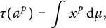
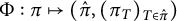 $$ \begin{align} \Phi:\pi \mapsto (\hat{\pi},(\pi_T)_{T \in \hat{\pi}}) \end{align} $$
is a bijection that will be used throughout the proof of Theorem 1.1; see Figure 3.
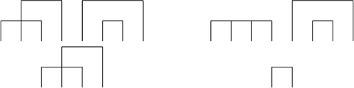
Figure 3: A partition
 $\pi $
and its image
$\pi $
and its image
 $\Phi (\pi )$
.
$\Phi (\pi )$
.
Note, for instance, that
 $|\hat {\pi }|=\mathbf {cc}(\pi )$
. We denote
$|\hat {\pi }|=\mathbf {cc}(\pi )$
. We denote
 $$ \begin{align*} \operatorname{Proj}(\hat{\pi}):=\{((\pi_T)_{T \in \hat{\pi}}): \pi_T \in P_2^{\operatorname{con}}(T), \ \forall T \in \hat{\pi}\}. \end{align*} $$
Given
 $a_1,\ldots ,a_n \in \mathcal {A}$
, we denote by
$a_1,\ldots ,a_n \in \mathcal {A}$
, we denote by
 $\kappa ^{\operatorname {free}}_n(a_1,\ldots ,a_n)$
their free cumulants, namely, for any
$\kappa ^{\operatorname {free}}_n(a_1,\ldots ,a_n)$
their free cumulants, namely, for any
 $i \in [n]^k$
, we have
$i \in [n]^k$
, we have
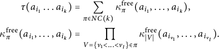 $$ \begin{align*} \tau(a_{i_1}\ldots a_{i_k}) & =\sum_{\pi \in NC(k)}\kappa^{\operatorname{free}}_\pi(a_{i_1},\ldots,a_{i_k}),\\ \kappa^{\operatorname{free}}_\pi(a_{i_1},\ldots,a_{i_k}) &=\prod_{V=\{v_1<\ldots<v_l\} \in \pi}\kappa^{\operatorname{free}}_{|V|}(a_{i_{v_1}},\ldots,a_{i_{v_l}}). \end{align*} $$
This is known as the moment–cumulant formula [Reference Nica and Speicher12, Notation 11.5]. Here and throughout the paper, we denote
 $V=\{v_1<\ldots <v_l\}$
a block
$V=\{v_1<\ldots <v_l\}$
a block
 $V=\{v_1,\ldots ,v_l\}$
such that
$V=\{v_1,\ldots ,v_l\}$
such that
 $v_1< \ldots <v_l$
; see [Reference Nica and Speicher12, Lecture 11]. Note also that if the variables
$v_1< \ldots <v_l$
; see [Reference Nica and Speicher12, Lecture 11]. Note also that if the variables
 $a_1,\ldots ,a_n$
are free, the free mixed cumulants vanish [Reference Nica and Speicher12, Proposition 11.15]. We denote
$a_1,\ldots ,a_n$
are free, the free mixed cumulants vanish [Reference Nica and Speicher12, Proposition 11.15]. We denote
 $\kappa ^{\operatorname {free}}_n(a)$
the free cumulants of a random variable a. The moment–cumulant formula implies the following, which is going to be used extensively in Subsection 5.3; see [Reference Nica and Speicher12, Lecture 5, Equation 5.6].
$\kappa ^{\operatorname {free}}_n(a)$
the free cumulants of a random variable a. The moment–cumulant formula implies the following, which is going to be used extensively in Subsection 5.3; see [Reference Nica and Speicher12, Lecture 5, Equation 5.6].
Lemma 2.1 Let
 $a,c_1,c_2$
be variables such that a is free from
$a,c_1,c_2$
be variables such that a is free from
 $\{c_1,c_2\}$
. Then
$\{c_1,c_2\}$
. Then
 $$ \begin{align*} \tau(ac_1ac_2)=\operatorname{var}(a)\tau(c_1)\tau(c_2)+\tau^2(a)\tau(c_1c_2). \end{align*} $$
We will equivalently denote
 $\kappa ^{\operatorname {free}}_n(\mu )$
the free cumulants of a random variable a with distribution
$\kappa ^{\operatorname {free}}_n(\mu )$
the free cumulants of a random variable a with distribution
 $\mu $
. Given two measures
$\mu $
. Given two measures
 $\mu _a$
and
$\mu _a$
and
 $\mu _b$
, the free convolution
$\mu _b$
, the free convolution
 $\mu _a \boxplus \mu _b$
denotes the distribution of
$\mu _a \boxplus \mu _b$
denotes the distribution of
 $a+b$
, where a and b are free random variables with distribution
$a+b$
, where a and b are free random variables with distribution
 $\mu _a$
and
$\mu _a$
and
 $\mu _b$
, respectively. The classical convolution
$\mu _b$
, respectively. The classical convolution
 $\mu _a+\mu _b$
denotes the distribution of
$\mu _a+\mu _b$
denotes the distribution of
 $a+b$
, where now a and b are classical independent random variables with distribution
$a+b$
, where now a and b are classical independent random variables with distribution
 $\mu _a$
and
$\mu _a$
and
 $\mu _b$
, respectively.
$\mu _b$
, respectively.
3 Properties of the limiting measure
In this section, we summarize some of the properties of the measure
 $\mu _q$
appearing in (3). We start by computing the free cumulants and the moments of
$\mu _q$
appearing in (3). We start by computing the free cumulants and the moments of
 $\mu _1$
.
$\mu _1$
.
Proposition 3.1 Let
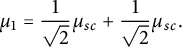 $$ \begin{align*} \mu_1=\frac{1}{\sqrt{2}}\mu_{sc}+\frac{1}{\sqrt{2}}\mu_{sc}. \end{align*} $$
Then the following hold.
-
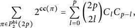
(1) Its odd moments vanish and, for every
 $p \in \mathbb {N}$
, its
$2p$
-th moment is given by where we recall that
$$ \begin{align*} \int x^{2p}\, \text{d}\mu_1&=2^{-p}\sum_{l=0}^p\binom{2p}{2l}C_lC_{p-l} =2^{-p}\sum_{\pi \in P_2^{\operatorname{bi}}(2p)}2^{\mathbf{cc}(\pi)}, \end{align*} $$
$C_l$
denotes the l-th Catalan number.
$p \in \mathbb {N}$
, its
$2p$
-th moment is given by where we recall that
$$ \begin{align*} \int x^{2p}\, \text{d}\mu_1&=2^{-p}\sum_{l=0}^p\binom{2p}{2l}C_lC_{p-l} =2^{-p}\sum_{\pi \in P_2^{\operatorname{bi}}(2p)}2^{\mathbf{cc}(\pi)}, \end{align*} $$
$C_l$
denotes the l-th Catalan number.
-
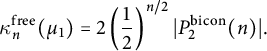
(2) Its odd free cumulants vanish,
$\kappa ^{\operatorname {free}}_2(\mu _1)=1$
and for any even integer
$n \ge 4$
, we have
$$ \begin{align*} \kappa^{\operatorname{free}}_n(\mu_1)=2\left(\frac{1}{2}\right)^{n/2}|P_2^{\operatorname{bicon}}(n)|. \end{align*} $$


Proof Let
 $x_1,x_2$
be two classical i.i.d semi-circle random variables. Then
$x_1,x_2$
be two classical i.i.d semi-circle random variables. Then
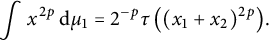 $$ \begin{align*} \int x^{2p}\, \text{d}\mu_1=2^{-p}\tau\left((x_1+x_2)^{2p}\right)\hspace{-1.5pt}. \end{align*} $$
Since the variables are classical independent, and in particular, they commute, we get
 $$ \begin{align*} \tau\left((x_1+x_2)^{2p}\right)=2^{-p}\sum_{l=0}^{2p}\binom{2p}{l}\tau(x_1^{l})\tau(x_2^{2p-l}). \end{align*} $$
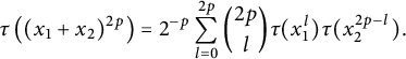
The odd moments of
 $x_1$
vanish and, for any
$x_1$
vanish and, for any
 $l \ge 1$
,
$l \ge 1$
,
 $\tau (x_1^{2l})=C_l$
, hence
$\tau (x_1^{2l})=C_l$
, hence
 $$ \begin{align*} \int x^{2p}\, \text{d}\mu_1=2^{-p}\sum_{l=0}^p\binom{2p}{2l}C_lC_{p-l}. \end{align*} $$
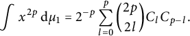
Now consider the sequence
 $m_p$
given by
$m_p$
given by
 $$ \begin{align*} m_p:=2^{-p}\sum_{\pi \in P_2^{\operatorname{bi}}(2p)}2^{\mathbf{cc}(\pi)}. \end{align*} $$
For every bipartite pair partition
 $\pi $
, we can decompose it into its bipartite sets. Namely, let
$\pi $
, we can decompose it into its bipartite sets. Namely, let
 $\mathcal {V}_1=\{V_1,\ldots , V_m\}$
and
$\mathcal {V}_1=\{V_1,\ldots , V_m\}$
and
 $\mathcal {V}_2=\{V_{m+1},\ldots , V_p\}$
be the bipartition of its blocks in two disjoint families of vertices. Then, the blocks
$\mathcal {V}_2=\{V_{m+1},\ldots , V_p\}$
be the bipartition of its blocks in two disjoint families of vertices. Then, the blocks
 $V_1,\ldots ,V_m$
are noncrossing from one another, and so are
$V_1,\ldots ,V_m$
are noncrossing from one another, and so are
 $V_{m+1},\ldots , V_p$
. Let
$V_{m+1},\ldots , V_p$
. Let
 $$ \begin{align*} I=\bigcup_{i=1}^m V_i \subseteq [2p]. \end{align*} $$
Then
 $$ \begin{align*} &\pi_1:=\{V_1,\ldots,V_m\} \in NC_2\left(I\right)\hspace{-1.5pt};\\ &\pi_2:=\{V_{m+1},\ldots,V_p\} \in NC_2\left(I^c\right)\hspace{-1.5pt}. \end{align*} $$
We denote
 $(\pi _1,\pi _2,I,I^c)$
a left-right noncrossing representation of
$(\pi _1,\pi _2,I,I^c)$
a left-right noncrossing representation of
 $\pi $
. We note that if
$\pi $
. We note that if
 $(\pi _1,\pi _2,I,I^c)$
is a left-right noncrossing representation of
$(\pi _1,\pi _2,I,I^c)$
is a left-right noncrossing representation of
 $\pi $
, so is
$\pi $
, so is
 $(\pi _2,\pi _1,I^c,I)$
. Let
$(\pi _2,\pi _1,I^c,I)$
. Let
 $R(\pi )$
be the set of all left-right noncrossing representations of
$R(\pi )$
be the set of all left-right noncrossing representations of
 $\pi $
. We note that
$\pi $
. We note that
 $|R(\pi )|$
corresponds to the number of ways the vertices of
$|R(\pi )|$
corresponds to the number of ways the vertices of
 $G(\pi )$
can be split into two independent families of vertices. Therefore, it is clear that
$G(\pi )$
can be split into two independent families of vertices. Therefore, it is clear that
 $$ \begin{align*} |R(\pi)|=2^{\mathbf{cc}(\pi)}. \end{align*} $$
Hence
 $$ \begin{align} \sum_{\pi \in P_2^{\operatorname{bi}}(2p)}2^{\mathbf{cc}(\pi)}=\sum_{\pi \in P_2^{\operatorname{bi}}(2p)}|R(\pi)|. \end{align} $$
Since
 $R(\pi )$
is the set of all left-right noncrossing representations of
$R(\pi )$
is the set of all left-right noncrossing representations of
 $\pi $
and we sum over all
$\pi $
and we sum over all
 $\pi \in P_2^{\operatorname {bi}}(2p)$
, we get
$\pi \in P_2^{\operatorname {bi}}(2p)$
, we get
 $$ \begin{align*} \sum_{\pi \in P_2^{\operatorname{bi}}(2p)}|R(\pi)|=|\{(\pi_1,\pi_2,I,I^c): I \subseteq[2p], \pi_1 \in NC_2(I),\pi_2 \in NC_2(I^c)\}|. \end{align*} $$
Note that for fixed
 $I \subseteq [2p]$
, each
$I \subseteq [2p]$
, each
 $(\pi _1,\pi _2) \in NC_2(I) \times NC_2(I^c)$
will correspond to a unique partition
$(\pi _1,\pi _2) \in NC_2(I) \times NC_2(I^c)$
will correspond to a unique partition
 $\pi \in P_2^{\operatorname {bi}}(2p)$
such that
$\pi \in P_2^{\operatorname {bi}}(2p)$
such that
 $(\pi _1,\pi _2,I,I^c)$
is a left-right noncrossing representation of
$(\pi _1,\pi _2,I,I^c)$
is a left-right noncrossing representation of
 $\pi $
. Hence we can first sum over
$\pi $
. Hence we can first sum over
 $I\subseteq [2p]$
so that
$I\subseteq [2p]$
so that
 $$ \begin{align*} \sum_{\pi \in P_2^{\operatorname{bi}}(2p)}|R(\pi)|=\sum_{I \subseteq [2p]}|\{(\pi_1,\pi_2): \pi_1 \in NC_2(I), \pi_2 \in NC_2(I^c)\}|. \end{align*} $$
Therefore, by (5), we have
 $$ \begin{align*} \sum_{\pi \in P_2^{\operatorname{bi}}(2p)}2^{\mathbf{cc}(\pi)}=\sum_{I \subseteq [2p]}|\{(\pi_1,\pi_2): \pi_1 \in NC_2(I), \pi_2 \in NC_2(I^c)\}|. \end{align*} $$
The latter cardinality can be written as a product over the cardinals and only depends on the length of I. More precisely, we have
 $$ \begin{align*} \sum_{\pi \in P_2^{\operatorname{bi}}(2p)}2^{\mathbf{cc}(\pi)}=\sum_{l=0}^p \binom{2p}{2l}C_lC_{p-l}, \end{align*} $$
where the cardinal
 $|NC_2(2l)|$
is equal to
$|NC_2(2l)|$
is equal to
 $C_l$
. Hence
$C_l$
. Hence
 $$ \begin{align*} \int x^{2p}\, \text{d}\mu_1=m_p, \end{align*} $$
and the first statement follows. For the second, we use the bijection
 $\Phi $
in (4) to write
$\Phi $
in (4) to write
 $\Phi (\pi )=\left (\hat {\pi },(\pi _T)_{T \in \hat {\pi }}\right )$
. We note that
$\Phi (\pi )=\left (\hat {\pi },(\pi _T)_{T \in \hat {\pi }}\right )$
. We note that
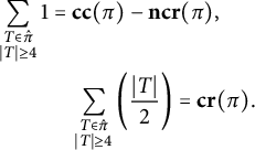 $$ \begin{align*} \sum_{\substack{T \in \hat{\pi}\\ |T| \ge 4}}1 &=\mathbf{cc}(\pi)-\mathbf{ncr}(\pi),\\ &\quad \sum_{\substack{T \in \hat{\pi}\\ |T| \ge 4}}\left(\frac{|T|}{2}\right) =\mathbf{cr}(\pi). \end{align*} $$
Hence
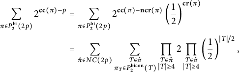 $$ \begin{align*} \sum_{\pi \in P_2^{\operatorname{bi}}(2p)}2^{\mathbf{cc}(\pi)-p}&=\sum_{\pi \in P_2^{\operatorname{bi}}(2p)}2^{\mathbf{cc}(\pi)-\mathbf{ ncr}(\pi)}\left(\frac{1}{2}\right)^{\mathbf{cr}(\pi)}\\ &=\sum_{\hat{\pi} \in NC(2p)}\sum_{\substack{T \in \hat{\pi}\\ \pi_T \in P_2^{\operatorname{bicon}}(T)}}\prod_{\substack{T \in \hat{\pi}\\ |T| \ge 4}}2 \prod_{\substack{T \in \hat{\pi}\\ |T| \ge 4}}\left(\frac{1}{2}\right)^{|T|/2}, \end{align*} $$
where we use that
 $\mathbf {ncr}(\pi )+\mathbf {cr}(\pi )=p$
in the first equality. We thus have
$\mathbf {ncr}(\pi )+\mathbf {cr}(\pi )=p$
in the first equality. We thus have
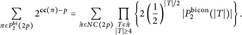 $$ \begin{align*} \sum_{\pi \in P_2^{\operatorname{bi}}(2p)}2^{\mathbf{cc}(\pi)-p}=\sum_{\hat{\pi} \in NC(2p)}\prod_{\substack{T \in \hat{\pi}\\ |T| \ge 4}}\left\{2\left(\frac{1}{2}\right)^{|T|/2}|P_2^{\operatorname{bicon}}(|T|)|\right\}. \end{align*} $$
Since the free cumulants
 $\kappa ^{\operatorname {free}}_n(\mu _1)$
are uniquely characterized by the moments, it follows that for any odd integer n, we have
$\kappa ^{\operatorname {free}}_n(\mu _1)$
are uniquely characterized by the moments, it follows that for any odd integer n, we have
 $\kappa ^{\operatorname {free}}_n(\mu _1)=0$
,
$\kappa ^{\operatorname {free}}_n(\mu _1)=0$
,
 $\kappa ^{\operatorname {free}}_2(\mu _1)=1$
and for any even integer
$\kappa ^{\operatorname {free}}_2(\mu _1)=1$
and for any even integer
 $n \ge 4$
, we have
$n \ge 4$
, we have
 $$ \begin{align*} \kappa^{\operatorname{free}}_n(\mu_1)=2\left(\frac{1}{2}\right)^{n/2}|P_2^{\operatorname{bicon}}(n)|. \end{align*} $$
Remark 3.2 For any
 $p \ge 1$
, it was shown in [Reference Gouyou-Beauchamps7] that
$p \ge 1$
, it was shown in [Reference Gouyou-Beauchamps7] that
 $$ \begin{align*} \sum_{l=0}^p \binom{2p}{2l}C_lC_{p-l}=C_pC_{p+1}. \end{align*} $$
Therefore, the
 $2p$
-th moment of
$2p$
-th moment of
 $\mu _1$
is also characterized by
$\mu _1$
is also characterized by
 $2^{-p}C_pC_{p+1}$
. The sequence
$2^{-p}C_pC_{p+1}$
. The sequence
 $(C_pC_{p+1})_{p \ge 1}$
is A005568 in Sloane’s encyclopedia (https://oeis.org/A005568), where several combinatorial objects counted by it are shown.
$(C_pC_{p+1})_{p \ge 1}$
is A005568 in Sloane’s encyclopedia (https://oeis.org/A005568), where several combinatorial objects counted by it are shown.
We are ready to compute the moments and free cumulants of
 $\mu _q$
.
$\mu _q$
.
Proposition 3.3 Given
 $q\in [0,1]$
, let
$q\in [0,1]$
, let
 $$ \begin{align*} \mu_q:=\sqrt{q}\left(\frac{1}{\sqrt{2}}\mu_{sc}+\frac{1}{\sqrt{2}}\mu_{sc}\right)\boxplus\sqrt{1-q}\, \mu_{sc}. \end{align*} $$
Then the following hold.
-
(1) The odd free cumulants of
$\mu _q$
vanish,
$\kappa ^{\operatorname {free}}_2(\mu _q)=1$
and for any even integer
$n \ge 4$
, we have
$$ \begin{align*} \kappa^{\operatorname{free}}_n(\mu_q)=2\Big(\frac{q}{2}\Big)^{n/2}|P_2^{\operatorname{bicon}}(n)|. \end{align*} $$
-
(2) The odd moments of
$\mu _q$
vanish and, for every
$p\in \mathbb {N}$
, its
$2p$
-th moment is given by
$$ \begin{align*} \sum_{\pi \in P_2^{\operatorname{bi}}(2p)}2^{\mathbf{cc}(\pi)-p}q^{\mathbf{cr}(\pi)}. \end{align*} $$


Proof We will use the notion of R-transform; see [Reference Nica and Speicher12, Lecture 16]. For a random variable
 $a \in \mathcal {A}$
with distribution
$a \in \mathcal {A}$
with distribution
 $\mu $
, let
$\mu $
, let
 $$ \begin{align*} R_a(z)=R_\mu(z)=\sum_{n \ge 1}\kappa^{\operatorname{free}}_n(a) z^n, \end{align*} $$
be its R-transform, defined as a formal series. The R-transform of a standard semi-circle law is given by
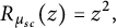 $$ \begin{align*} R_{\mu_{sc}}(z)=z^2, \end{align*} $$
whereas Proposition 3.1 shows that the R-transform of
 $\mu _1$
is given by
$\mu _1$
is given by
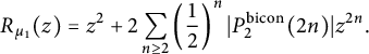 $$ \begin{align*} R_{\mu_1}(z)=z^2+2\sum_{n \ge 2}\left(\frac{1}{2}\right)^{n}|P_2^{\operatorname{bicon}}(2n)|z^{2n}. \end{align*} $$
Since the free cumulants linearize the free convolution, we deduce that
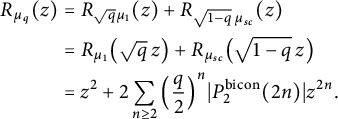 $$ \begin{align*} R_{\mu_q}(z)&= R_{\sqrt{q}\mu_1}(z)+ R_{\sqrt{1-q} \,\mu_{sc}}(z) \\ & = R_{\mu_1}\big(\sqrt{q}\,z\big) + R_{\mu_{sc}}\big(\sqrt{1-q} \,z\big)\\ &= z^2+ 2\sum_{n\ge 2} \Big(\frac{q}{2}\Big)^{n}|P_2^{\operatorname{bicon}}(2n)|z^{2n}. \end{align*} $$
This proves the first part of the proposition. To prove the second part, we use the moment–cumulant formula to deduce that the odd moments vanish, while the
 $2p$
-th moment can be expressed as
$2p$
-th moment can be expressed as
 $$ \begin{align*} \sum_{\hat{\pi}\in NC(2p)}\prod_{T \in \hat{\pi}} \kappa^{\operatorname{free}}_{|T|}(\mu_q) &=\sum_{\hat{\pi}\in NC(2p)}\prod_{\underset{|T|\geq 4}{T \in \hat{\pi}}}\left\{ 2\Big(\frac{q}{2}\Big)^{|T|/2}|P_2^{\operatorname{bicon}}(T)|\right\}\\ &=\sum_{\hat{\pi}\in NC(2p)}\sum_{(\pi_T)_{T \in \hat{\pi}}}\prod_{\underset{|T|\geq 4}{T \in \hat{\pi}}} \left\{2\Big(\frac{q}{2}\Big)^{|T|/2}\right\},\\ \end{align*} $$
where the second summation is over
 $(\pi _T)_{T \in \hat {\pi }} \in \operatorname {Proj}(\hat {\pi })$
such that
$(\pi _T)_{T \in \hat {\pi }} \in \operatorname {Proj}(\hat {\pi })$
such that
 $\pi _T \in P_2^{\operatorname {bicon}}(T)$
for
$\pi _T \in P_2^{\operatorname {bicon}}(T)$
for
 $T \in \hat {\pi }$
. Now noting that
$T \in \hat {\pi }$
. Now noting that
 $$ \begin{align*} &|\{T \in \hat{\pi}:|T| \ge 4\}|=\mathbf{cc}(\pi)-\mathbf{ncr}(\pi), \end{align*} $$
and
 $$ \begin{align*}\sum_{\substack{T \in \hat{\pi}\\ |T| \ge 4}}\frac{|T|}{2}=\mathbf{cr}(\pi), \end{align*} $$
we finish the proof after using the bijection
 $\Phi $
from (4) to rewrite the above expression.
$\Phi $
from (4) to rewrite the above expression.
4 Existence of the limit
The goal of this section is to show that the expression in (1) admits a limit that depends only on the first and second moments of the variables at hand. Let us first prove the following centering lemma.
Lemma 4.1 Let
 $(\mathcal {A},\tau )$
be a unital faithful tracial noncommutative probability space. Let
$(\mathcal {A},\tau )$
be a unital faithful tracial noncommutative probability space. Let
 $\{a_k: k \in [n]\},\{d_k: k \in [n]\} \subset \mathcal {A}$
be two collections of free random variables and let
$\{a_k: k \in [n]\},\{d_k: k \in [n]\} \subset \mathcal {A}$
be two collections of free random variables and let
 $$ \begin{align*} c_k:=a_k\otimes d_k-\tau\otimes \tau(a_k\otimes d_k), \end{align*} $$
for every
 $k\in [n]$
. Then for any
$k\in [n]$
. Then for any
 $m \ge 1$
and
$m \ge 1$
and
 $i_1,\ldots ,i_m \in [n]$
such that there exists an index
$i_1,\ldots ,i_m \in [n]$
such that there exists an index
 $l^* \in [m]$
satisfying
$l^* \in [m]$
satisfying
 $i_{l^*} \ne i_j$
for all
$i_{l^*} \ne i_j$
for all
 $j \ne l^*$
, we have
$j \ne l^*$
, we have
 $$ \begin{align*} \tau\otimes \tau(c_{i_1}\ldots c_{i_{m}})=0. \end{align*} $$
In particular, we have
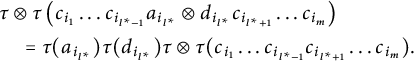 $$ \begin{align*} & \tau\otimes \tau\left(c_{i_1}\ldots c_{i_{l^*-1}}a_{i_{l^*}}\otimes d_{i_{l^*}} c_{i_{l^*+1}}\ldots c_{i_m} \right) \\ &\quad =\tau(a_{i_{l^*}})\tau(d_{i_{l^*}})\tau\otimes \tau(c_{i_1}\ldots c_{i_{l^*-1}} c_{i_{l^*+1}}\ldots c_{i_m}). \end{align*} $$
Proof By cyclicity of the trace, we can assume that
 $l^*=1$
. We write
$l^*=1$
. We write
 $$ \begin{align} \tau\otimes \tau(c_{i_1}\ldots c_{i_m})=\tau\otimes \tau(a_{i_1}\otimes d_{i_1}c_{i_2}\ldots c_{i_m})-\tau\otimes \tau(a_{i_1}\otimes d_{i_1})\tau\otimes \tau(c_{i_2}\ldots c_{i_m}). \end{align} $$
For the first term, we open the expressions for
 $c_{i_j}$
for
$c_{i_j}$
for
 $j \ge 2$
to get that
$j \ge 2$
to get that
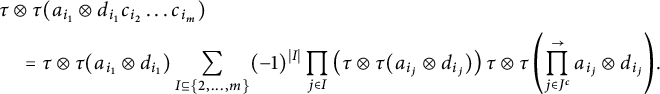
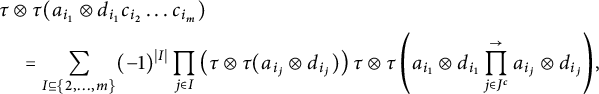 $$ \begin{align*} &\tau\otimes \tau(a_{i_1}\otimes d_{i_1}c_{i_2}\ldots c_{i_m}) \\ &\quad =\sum_{I\subseteq \{2,\ldots,m\}}(-1)^{|I|}\prod_{j \in I}\left(\tau\otimes \tau(a_{i_j}\otimes d_{i_j}) \right)\tau\otimes \tau\left(a_{i_1}\otimes d_{i_1}\prod_{j \in J^c}^{\to}a_{i_j}\otimes d_{i_j}\right)\hspace{-1.5pt}, \end{align*} $$
where
 $\overset {\to }{\prod }$
denotes the product respecting the ordering. Since
$\overset {\to }{\prod }$
denotes the product respecting the ordering. Since
 $a_{i_1},d_{i_1}$
are free from
$a_{i_1},d_{i_1}$
are free from
 $a_{i_j},d_{i_j}$
for all
$a_{i_j},d_{i_j}$
for all
 $j \ge 2$
, freeness implies that
$j \ge 2$
, freeness implies that
 $$ \begin{align*} &\tau\otimes \tau(a_{i_1}\otimes d_{i_1}c_{i_2}\ldots c_{i_m})\\ &\quad =\tau\otimes \tau(a_{i_1}\otimes d_{i_1})\sum_{I\subseteq \{2,\ldots,m\}}(-1)^{|I|}\prod_{j \in I}\left(\tau\otimes \tau(a_{i_j}\otimes d_{i_j})\right) \tau\otimes \tau\left(\prod_{j \in J^c}^{\to}a_{i_j}\otimes d_{i_j}\right)\hspace{-1.5pt}. \end{align*} $$
The summation can be easily written as
 $\tau \otimes \tau (c_{i_2}\ldots c_{i_m})$
, hence
$\tau \otimes \tau (c_{i_2}\ldots c_{i_m})$
, hence
 $$ \begin{align*} \tau\otimes \tau(a_{i_1}\otimes d_{i_1}c_{i_2}\ldots c_{i_m})=\tau\otimes \tau(a_{i_1}\otimes d_{i_1})\tau\otimes \tau(c_{i_2}\ldots c_{i_m}). \end{align*} $$
By (6), we then have
 $$ \begin{align*} \tau\otimes \tau(c_{i_1}\ldots c_{i_m})=0. \end{align*} $$
Finally, since
 $\tau \otimes \tau (a_{i_1}\otimes d_{i_1})=\tau (a_{i_1})\tau (d_{i_1})$
, we get that
$\tau \otimes \tau (a_{i_1}\otimes d_{i_1})=\tau (a_{i_1})\tau (d_{i_1})$
, we get that
 $$ \begin{align*} \tau\otimes \tau(a_{i_1}\otimes d_{i_1}c_{i_2}\ldots c_{i_m})&=\tau\otimes \tau(a_{i_1}\otimes d_{i_1})\tau\otimes \tau(c_{i_2}\ldots c_{i_m})\\ &=\tau(a_{i_1})\tau(d_{i_1})\tau\otimes \tau(c_{i_2}\ldots c_{i_m}). \end{align*} $$
We are now ready to prove the existence of the limit and that it only depends on the first and second moments of the
 $a_k$
’s. It also follows from a general scheme to prove a Central Limit Theorem type-result of Boejko and Speicher [Reference Bożejko and Speicher3, Theorem 0]. For
$a_k$
’s. It also follows from a general scheme to prove a Central Limit Theorem type-result of Boejko and Speicher [Reference Bożejko and Speicher3, Theorem 0]. For
 $i\in [n]^p$
, we denote
$i\in [n]^p$
, we denote
 $\ker i\in P(p)$
the partition such that
$\ker i\in P(p)$
the partition such that
 $k,l$
are in the same block of
$k,l$
are in the same block of
 $\ker i$
if and only if
$\ker i$
if and only if
 $i_j=i_k$
.
$i_j=i_k$
.
Proposition 4.2 (Existence)
Let
 $(a_n)_{n\in \mathbb {N}} \in (\mathcal {A},\tau )$
be free self-adjoint identically distributed random variables with mean
$(a_n)_{n\in \mathbb {N}} \in (\mathcal {A},\tau )$
be free self-adjoint identically distributed random variables with mean
 $\lambda $
, variance
$\lambda $
, variance
 $\sigma ^2$
, and denote
$\sigma ^2$
, and denote
 $\delta ^2:=\operatorname {var}(a_1\otimes a_1)= \sigma ^2(\sigma ^2+2\lambda ^2)$
. For every
$\delta ^2:=\operatorname {var}(a_1\otimes a_1)= \sigma ^2(\sigma ^2+2\lambda ^2)$
. For every
 $k\in \mathbb {N}$
, denote
$k\in \mathbb {N}$
, denote
 $$ \begin{align*} b_k:=\frac{1}{\delta}\big(a_k\otimes a_k-\tau\otimes \tau(a_k\otimes a_k)\big), \end{align*} $$
and for every
 $n\in \mathbb {N}$
, denote
$n\in \mathbb {N}$
, denote
 $$ \begin{align*} S_n:=\frac{1}{\sqrt{n}}\sum_{k \in [n]}b_k. \end{align*} $$
Then there exists a random variable
 $\mathbf {{S}} \in (\mathcal {A}',\tau ')$
such that
$\mathbf {{S}} \in (\mathcal {A}',\tau ')$
such that
 $S_n\Rightarrow \mathbf {{S}}$
. Moreover, the law of
$S_n\Rightarrow \mathbf {{S}}$
. Moreover, the law of
 $\mathbf {{S}}$
depends only on
$\mathbf {{S}}$
depends only on
 $\lambda $
and
$\lambda $
and
 $\sigma $
, its odd moments vanish and, for every
$\sigma $
, its odd moments vanish and, for every
 $p\in \mathbb {N}$
,
$p\in \mathbb {N}$
,
 $$ \begin{align*} \tau'(\mathbf{{S}}^{2p})=\sum_{\pi \in P_2(2p)}\tau\otimes \tau(b_{i_1}\ldots b_{i_{2p}}), \end{align*} $$
where
 $i \in [p]^{2p}$
is any sequence such that
$i \in [p]^{2p}$
is any sequence such that
 $\ker i=\pi $
.
$\ker i=\pi $
.
Proof We begin by writing
 $$ \begin{align*} \tau\otimes \tau(S_n^p)=\frac{1}{n^{p/2}}\sum_{i \in [n]^p}\tau\otimes \tau (b_{i_1}\ldots b_{i_p}). \end{align*} $$
Since
 $b_{1},\ldots ,b_n$
are identically distributed, the expression
$b_{1},\ldots ,b_n$
are identically distributed, the expression
 $$ \begin{align} \tau\otimes \tau (b_{i_1}\ldots b_{i_p}) \end{align} $$
depends only on the partition
 $\pi =\ker i \in P(p)$
. Denote the common value of (7) by
$\pi =\ker i \in P(p)$
. Denote the common value of (7) by
 $\tau \otimes \tau (\pi )$
. Then we have
$\tau \otimes \tau (\pi )$
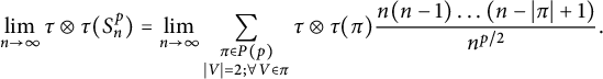
. Then we have
 $$ \begin{align*} \tau\otimes \tau(S_n^p)=\frac{1}{n^{p/2}}\sum_{\pi \in P(p)}\tau\otimes \tau(\pi)|\{i \in [n]^p: \pi(i)=\pi\}|. \end{align*} $$
To count the cardinality, we choose an index for each block. Therefore, we have
 $$ \begin{align*} |\{i \in [n]^p: \pi(i)=\pi\}|=n(n-1)\ldots (n-|\pi|+1) \sim n^{|\pi|}. \end{align*} $$
By Lemma 4.1, if
 $\pi $
has a block of size
$\pi $
has a block of size
 $1$
,
$1$
,
 $\tau \otimes \tau (\pi )=0$
. Thus, we have
$\tau \otimes \tau (\pi )=0$
. Thus, we have
 $$ \begin{align*} \tau\otimes \tau(S_n^p)=\sum_{\substack{\pi \in P(p)\\ |V| \ge 2; \forall V \in \pi}}\tau\otimes \tau(\pi)\frac{n(n-1)\ldots (n-|\pi|+1) }{n^{p/2}}. \end{align*} $$
Since
 $|V| \ge 2$
for all blocks
$|V| \ge 2$
for all blocks
 $V \in \pi $
, we have
$V \in \pi $
, we have
 $|\pi | \le p/2$
. If there exists a block
$|\pi | \le p/2$
. If there exists a block
 $V \in \pi $
such that
$V \in \pi $
such that
 $|V| \ge 3$
, we immediately have
$|V| \ge 3$
, we immediately have
 $|\pi |<p/2$
, and its contribution is negligible. In particular, this implies that the odd moments of
$|\pi |<p/2$
, and its contribution is negligible. In particular, this implies that the odd moments of
 $S_n$
are asymptotically vanishing. We deduce that
$S_n$
are asymptotically vanishing. We deduce that
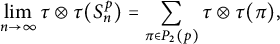
 $$ \begin{align*} \lim_{n \to \infty}\tau\otimes \tau(S_n^p)=\lim_{n\to \infty}\sum_{\substack{\pi \in P(p)\\ |V| = 2; \forall V \in \pi}}\tau\otimes \tau(\pi)\frac{n(n-1)\ldots (n-|\pi|+1) }{n^{p/2}}. \end{align*} $$
In this case,
 $\pi $
is a pair partition and
$\pi $
is a pair partition and
 $|\pi |=p/2$
, hence we deduce the formula
$|\pi |=p/2$
, hence we deduce the formula
 $$ \begin{align*} \lim_{n \to \infty}\tau\otimes \tau(S_n^p)=\sum_{\pi \in P_2(p)}\tau\otimes \tau(\pi), \end{align*} $$
which shows that
 $S_n$
converges. To prove that the limit depends only on
$S_n$
converges. To prove that the limit depends only on
 $\lambda $
and
$\lambda $
and
 $\sigma $
, we write
$\sigma $
, we write
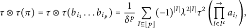 $$ \begin{align*} \tau\otimes \tau(\pi)=\tau\otimes \tau(b_{i_1}\ldots b_{i_p})=\frac{1}{\delta^p}\sum_{I \subseteq [p]}(-1)^{|I|}\lambda^{2|I|}\tau^2\left(\prod_{l \in I^c}^{\to}a_{i_l}\right)\hspace{-1.5pt}, \end{align*} $$
where
 $\pi (i)=\pi $
. By the moment–cumulant formula, we have
$\pi (i)=\pi $
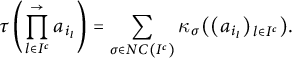
. By the moment–cumulant formula, we have
 $$ \begin{align*} \tau\left(\prod_{l \in I^c}^{\to}a_{i_l}\right)=\sum_{\sigma \in NC(I^c)} \kappa_\sigma((a_{i_l})_{l \in I^c}). \end{align*} $$
Since the mixed cumulants of free variables vanish, the only partitions
 $\sigma \in NC(I^c)$
that contribute are those such that every block
$\sigma \in NC(I^c)$
that contribute are those such that every block
 $V \in \sigma $
has cardinality at most two. We then have
$V \in \sigma $
has cardinality at most two. We then have
 $$ \begin{align*} \kappa_\sigma((a_{i_l})_{l \in I^c})&=\prod_{\substack{V \in \sigma\\ |V|=2}}\kappa_{|V|}(a,a)\prod_{\substack{V \in \sigma\\ |V|=1}}\kappa_{|V|}(a) =\sigma^{2\#\{V \in \sigma:|V|=2\}}\lambda^{\#\{V \in \sigma:|V|=1\}}. \end{align*} $$
This concludes the proof.
5 Proof of Theorem 1.1
After proving the existence of the limit in the previous section, the goal here is to identify this limit as stated in Theorem 1.1. In all this section,
 $(a_n)_{n\in \mathbb {N}}$
denote free copies of a random variable a with mean
$(a_n)_{n\in \mathbb {N}}$
denote free copies of a random variable a with mean
 $\lambda $
and variance
$\lambda $
and variance
 $\sigma ^2$
. Moreover, the common law of the normalized tensors will be denoted by
$\sigma ^2$
. Moreover, the common law of the normalized tensors will be denoted by
 $$ \begin{align} b=\frac{1}{\delta}\big(a\otimes a-\lambda^2\big), \end{align} $$
where
 $\delta ^2=\operatorname {var}(a\otimes a)=\sigma ^2(\sigma ^2+2\lambda ^2)$
.
$\delta ^2=\operatorname {var}(a\otimes a)=\sigma ^2(\sigma ^2+2\lambda ^2)$
.
Throughout the proof, we will assume p is an even integer. Following Proposition 4.2, we denote
 $\mathbf {{S}}$
the limit of
$\mathbf {{S}}$
the limit of
 $S_n$
and note that
$S_n$
and note that
 $$ \begin{align*} \tau'(\mathbf{{S}}^{p})=\sum_{\pi \in P_2(p)}\tau\otimes \tau(\pi), \end{align*} $$
where
 $\tau \otimes \tau (\pi )=\tau \otimes \tau (b_{i_1}\ldots b_{i_p})$
with
$\tau \otimes \tau (\pi )=\tau \otimes \tau (b_{i_1}\ldots b_{i_p})$
with
 $\pi (i)=\pi $
.
$\pi (i)=\pi $
.
5.1 Contribution of noncrossing blocks
We begin by removing interval blocks.
Lemma 5.1 Let
 $\pi \in P_2(p)$
and suppose that there exists
$\pi \in P_2(p)$
and suppose that there exists
 $l \in [p]$
such that
$l \in [p]$
such that
 $\{l,l+1\} \in \pi $
(with the convention that
$\{l,l+1\} \in \pi $
(with the convention that
 $p+1:=1$
). Then
$p+1:=1$
). Then
 $$ \begin{align*} \tau \otimes \tau (\pi)=\tau\otimes \tau(\pi\setminus \{l,l+1\}). \end{align*} $$
Proof By cyclicity, we can assume
 $l=p-1$
. We then have
$l=p-1$
. We then have
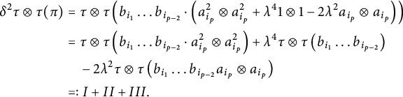 $$ \begin{align*} \delta^2 \tau\otimes \tau(\pi)&=\tau\otimes \tau\left(b_{i_1}\ldots b_{i_{p-2}}\cdot \left(a_{i_p}^2\otimes a_{i_p}^2+\lambda^41\otimes 1-2\lambda^2a_{i_p}\otimes a_{i_p}\right)\right)\\ &=\tau\otimes \tau\left(b_{i_1}\ldots b_{i_{p-2}}\cdot a_{i_p}^2\otimes a_{i_p}^2\right)+\lambda^4\tau\otimes \tau\left(b_{i_1}\ldots b_{i_{p-2}}\right)\\ &\quad -2\lambda^2\tau\otimes \tau\left(b_{i_1}\ldots b_{i_{p-2}}a_{i_p}\otimes a_{i_p}\right)\\ &=:I+II+III. \end{align*} $$
We immediately recognize
 $$ \begin{align*} II=\lambda^4\tau\otimes \tau(\pi\setminus \{p-1,p\}). \end{align*} $$
By Lemma 4.1, we have
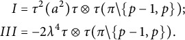 $$ \begin{align*} I & =\tau^2(a^2)\tau\otimes \tau(\pi\setminus \{p-1,p\});\\ III & =-2\lambda^4\tau\otimes \tau(\pi\setminus \{p-1,p\}). \end{align*} $$
Hence
 $$ \begin{align*} \delta^2\tau\otimes \tau(\pi)=\left(\tau^2(a^2)-\lambda^4\right)\tau\otimes \tau(\pi\setminus \{p-1,p\}). \end{align*} $$
To conclude, we note that
 $\tau ^2(a^2)-\lambda ^4=\delta ^2$
and finish the proof.
$\tau ^2(a^2)-\lambda ^4=\delta ^2$
and finish the proof.
Recall that a noncrossing pair partition
 $\pi \in NC_2(p)$
always has an interval block
$\pi \in NC_2(p)$
always has an interval block
 $V=\{l,l+1\} \in \pi $
such that
$V=\{l,l+1\} \in \pi $
such that
 $\pi \setminus V$
is a noncrossing pair partition. In particular, by induction, Lemma 5.1 implies the following.
$\pi \setminus V$
is a noncrossing pair partition. In particular, by induction, Lemma 5.1 implies the following.
Corollary 5.2 For any
 $\pi \in NC_2(p)$
, we have
$\pi \in NC_2(p)$
, we have
 $\tau \otimes \tau (\pi )=1$
.
$\tau \otimes \tau (\pi )=1$
.
5.2 Decomposition of pair partitions
In order to capture the contribution of crossing partitions, we need to decompose a partition
 $\pi \in P_2(p)\setminus NC_2(p)$
using smaller partitions. We denote
$\pi \in P_2(p)\setminus NC_2(p)$
using smaller partitions. We denote
 $\pi =\pi _1\oplus \ldots \oplus \pi _k$
if
$\pi =\pi _1\oplus \ldots \oplus \pi _k$
if
 $[p]$
can be decomposed into k intervals
$[p]$
can be decomposed into k intervals
 $I_1,\ldots ,I_k$
such that
$I_1,\ldots ,I_k$
such that
 $\pi _k \in P_2(I_k)$
and
$\pi _k \in P_2(I_k)$
and
 $V \in \pi $
if
$V \in \pi $
if
 $V \in \pi _l$
for some
$V \in \pi _l$
for some
 $1 \le l \le k$
. For
$1 \le l \le k$
. For
 $I \subseteq [p]$
, let
$I \subseteq [p]$
, let
 $$ \begin{align} a_I:=\prod_{l \in I}^{\to}a_{i_l}, \end{align} $$
and
 $a_{\varnothing }:=1$
.
$a_{\varnothing }:=1$
.
Lemma 5.3 Let
 $\pi \in P_2(p)$
. Then, the following hold.
$\pi \in P_2(p)$
. Then, the following hold.
-
(5.3.i) If
$\pi =\pi _1 \oplus \ldots \oplus \pi _l$
, then
$$ \begin{align*} \tau\otimes \tau(\pi)=\tau\otimes \tau(\pi_1)\ldots \tau\otimes \tau(\pi_l). \end{align*} $$
-
(5.3.ii) If
$\pi =\{1,p\}\cup \pi _1$
, where
$\pi _1 \in P_2(\{2,\ldots ,p-1\})$
, then
$$ \begin{align*} \tau\otimes \tau(\pi)=\tau\otimes \tau(\pi_1). \end{align*} $$
Moreover, if there exists an interval
$I \subseteq [p]$
such that
$\pi |_I$
is a pair partition, then
$$ \begin{align*} \tau\otimes \tau(\pi)=\tau\otimes \tau(\pi|_I)\tau\otimes \tau (\pi|_{I^c}). \end{align*} $$
-
(5.3.iii) If
$\pi $
has a block
$V=\{r,s\}$
such that for any block
$U=\{l,k\} \in \pi $
with
$r <l<s$
, we have
$r<k<s$
(i.e., every point inside V matches another one inside V), we have where
$$ \begin{align*} \tau\otimes \tau(\pi)=\tau\otimes \tau(\pi|_{V_-})\tau\otimes \tau(\pi|_{V_+}), \end{align*} $$
$\pi |_{V_-}$
is the restriction of
$\pi $
to inside of V and
$\pi |_{V_+}$
is the restriction of
$\pi $
to outside of V.


Proof
(5.3.i) By induction, it suffices to prove the case
 $\pi =\pi _1\oplus \pi _2$
. Let
$\pi =\pi _1\oplus \pi _2$
. Let
 $I_1,I_2$
be the disjoint decomposition of
$I_1,I_2$
be the disjoint decomposition of
 $[p]$
given by
$[p]$
given by
 $\pi _1$
and
$\pi _1$
and
 $\pi _2$
. Then, we can write
$\pi _2$
. Then, we can write
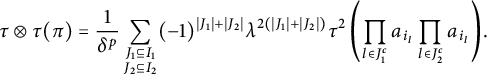 $$ \begin{align*} \tau\otimes \tau(\pi)=\frac{1}{\delta^p}\sum_{\substack{J_1 \subseteq I_1\\ J_2 \subseteq I_2}}(-1)^{|J_1|+|J_2|}\lambda^{2(|J_1|+|J_2|)}\tau^2\left(\prod_{l \in J_1^c}a_{i_l}\prod_{l \in J_2^c}a_{i_l}\right)\hspace{-1.5pt}. \end{align*} $$
Since
 $\pi $
is the direct sum of
$\pi $
is the direct sum of
 $\pi _1,\pi _2$
, the variables
$\pi _1,\pi _2$
, the variables
 $a_{J_1^c}, a_{J_2^c}$
are free and we can write
$a_{J_1^c}, a_{J_2^c}$
are free and we can write
 $$ \begin{align*} \tau\otimes \tau(\pi)=\frac{1}{\delta^p}\sum_{\substack{J_1 \subseteq I_1\\ J_2 \subseteq I_2}}(-1)^{|J_1|+|J_2|}\lambda^{2(|J_1|+|J_2|)}\tau^2\left(\prod_{l \in J_1^c}a_{i_l}\right)\tau^2\left(\prod_{l \in J_2^c}a_{i_l}\right)\hspace{-1.5pt}. \end{align*} $$
It is immediate to check that the right-hand-side is equal to
 $\tau \otimes \tau (\pi _1)\tau \otimes \tau (\pi _2)$
.
$\tau \otimes \tau (\pi _1)\tau \otimes \tau (\pi _2)$
.
(5.3.ii) By cyclicity, we have
 $$ \begin{align*} \tau\otimes \tau(\pi)&=\tau\otimes \tau(b_{i_2}\ldots b_{i_{p-1}}b_{i_{p}}b_{i_1}). \end{align*} $$
Since
 $\{1,p\} \in \pi $
, Lemma 5.1 implies that
$\{1,p\} \in \pi $
, Lemma 5.1 implies that
 $$ \begin{align*} \tau\otimes \tau(\pi)=\tau\otimes \tau(b_{i_2}\ldots b_{i_{p-1}})=\tau\otimes \tau(\pi_1). \end{align*} $$
The second part follows again by cyclicity as we can assume
 $I=\{1,\ldots ,k\}$
for some
$I=\{1,\ldots ,k\}$
for some
 $k \in [p]$
, and the variables are free.
$k \in [p]$
, and the variables are free.
(5.3.iii) By cyclicity, we can assume that
 $V=\{1,k\}$
for some
$V=\{1,k\}$
for some
 $k\in [p]$
. Note that V creates a direct sum
$k\in [p]$
. Note that V creates a direct sum
 $\pi =(V\cup \pi |_{V_-})\oplus \pi |_{V_+}$
. The result follows by (5.3.i) and (5.3.ii).
$\pi =(V\cup \pi |_{V_-})\oplus \pi |_{V_+}$
. The result follows by (5.3.i) and (5.3.ii).
Note that any block
 $V \in \pi $
that does not cross any other block of
$V \in \pi $
that does not cross any other block of
 $\pi $
is either an interval block or a block that satisfies (5.3.iii). In particular, its removal does not affect the value of
$\pi $
is either an interval block or a block that satisfies (5.3.iii). In particular, its removal does not affect the value of
 $\tau \otimes \tau (\pi )$
. It is clear then that
$\tau \otimes \tau (\pi )$
. It is clear then that
 $\tau \otimes \tau (\pi )$
is a multiplicative function [Reference Bożejko and Speicher4] over the connected components of
$\tau \otimes \tau (\pi )$
is a multiplicative function [Reference Bożejko and Speicher4] over the connected components of
 $\pi $
. Using the mapping
$\pi $
. Using the mapping
 $\Phi $
defined in (4), we can write
$\Phi $
defined in (4), we can write
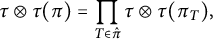 $$ \begin{align} \tau\otimes \tau(\pi)=\prod_{T \in \hat{\pi}}\tau\otimes \tau (\pi_T), \end{align} $$
where
 $(\hat {\pi },(\pi _T)_{T \in \hat {\pi }})=\Phi (\pi )$
. In view of this, we will now focus on the case where
$(\hat {\pi },(\pi _T)_{T \in \hat {\pi }})=\Phi (\pi )$
. In view of this, we will now focus on the case where
 $\pi \in P_2^{\operatorname {con}}(p)$
, for
$\pi \in P_2^{\operatorname {con}}(p)$
, for
 $p \ge 4$
, as the case
$p \ge 4$
, as the case
 $p=2$
corresponds to noncrossing blocks.
$p=2$
corresponds to noncrossing blocks.
5.3 Contribution of connected partitions
Given
 $\pi \in P_2^{\operatorname {con}}(p)$
, for an even integer
$\pi \in P_2^{\operatorname {con}}(p)$
, for an even integer
 $p \ge 4$
, we recall that
$p \ge 4$
, we recall that
 $\pi \in P_2^{\operatorname {bicon}}(p)$
if its intersection graph
$\pi \in P_2^{\operatorname {bicon}}(p)$
if its intersection graph
 $G(\pi )$
is a bipartite connected graph.
$G(\pi )$
is a bipartite connected graph.
The following is the main proposition of this subsection.
Proposition 5.4 Let
 $p \ge 4$
be an even integer and
$p \ge 4$
be an even integer and
 $\pi \in P_2^{\operatorname {con}}(p)$
. Then the following hold.
$\pi \in P_2^{\operatorname {con}}(p)$
. Then the following hold.
-
(1) If
$\pi \notin P_2^{\operatorname {bicon}}(p)$
, then
$\tau \otimes \tau (\pi )=0$
; -
(2) If
$\pi \in P_2^{\operatorname {bicon}}(p)$
, then where
$$ \begin{align*} \tau\otimes \tau(\pi)=2 \Big(\frac{q}{2}\Big)^{\frac{p}{2}}, \end{align*} $$
$q=\frac {2\lambda ^2}{\sigma ^2+2\lambda ^2}$
.


To prove Proposition 5.4, our goal is to remove the blocks
 $V \in \pi $
one at a time and track its influence on the rest of the partition
$V \in \pi $
one at a time and track its influence on the rest of the partition
 $\pi \setminus V$
. To this end, we will define two main quantities associated with V. First, we will define a coloring
$\pi \setminus V$
. To this end, we will define two main quantities associated with V. First, we will define a coloring
 $w_V \in \{0,1\}$
of V that encodes how the removal of V affects the other blocks. Secondly, we will define a binary vector
$w_V \in \{0,1\}$
of V that encodes how the removal of V affects the other blocks. Secondly, we will define a binary vector
 $\theta _V \in \{0,1\}^4$
satisfying
$\theta _V \in \{0,1\}^4$
satisfying
 $$ \begin{align*} \sum_{j\in[4]} \theta_j=1, \end{align*} $$
that is, only one coordinate of
 $\theta _V$
is equal to
$\theta _V$
is equal to
 $1$
. It encodes how we remove the block V from
$1$
. It encodes how we remove the block V from
 $\pi $
, that is, its weight to
$\pi $
, that is, its weight to
 $\tau \otimes \tau (\pi )$
. Let us begin this description now.
$\tau \otimes \tau (\pi )$
. Let us begin this description now.
Let
 $\pi \in P_2^{\operatorname {con}}(p)$
and
$\pi \in P_2^{\operatorname {con}}(p)$
and
 $i \in [p]^p$
such that
$i \in [p]^p$
such that
 $\pi (i)=\pi $
. Given an integer
$\pi (i)=\pi $
. Given an integer
 $t \ge 0$
, blocks
$t \ge 0$
, blocks
 $V_1,\ldots ,V_t,V_{t+1} \in \pi $
, and a coloring
$V_1,\ldots ,V_t,V_{t+1} \in \pi $
, and a coloring
 $w \in \{0,1\}^{t+1}$
, we denote
$w \in \{0,1\}^{t+1}$
, we denote
 $V_j^{(w_j)}$
the block
$V_j^{(w_j)}$
the block
 $V_j$
under the color
$V_j$
under the color
 $w_j$
. We then define the iterated joint law of
$w_j$
. We then define the iterated joint law of
 $b_{i_j}$
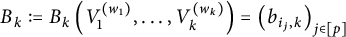 $$ \begin{align*} B_k:=B_k\left(V_1^{(w_1)},\ldots, V_k^{(w_k)}\right)=\left(b_{i_j,k}\right)_{j \in [p]} \end{align*} $$
for
 $k \le t+1$
as follows. Let
$k \le t+1$
as follows. Let
 $(\tilde {a}_j)_{j \in \mathbb {N}}$
be a family of free copies of a, free from
$(\tilde {a}_j)_{j \in \mathbb {N}}$
be a family of free copies of a, free from
 $(a_j)_{j \in \mathbb {N}}$
. For
$(a_j)_{j \in \mathbb {N}}$
. For
 $k=0$
, we define
$k=0$
, we define
 $B_0=(b_{i_j})_{j \in [p]}$
and for any
$B_0=(b_{i_j})_{j \in [p]}$
and for any
 $1 \le k \le t+1$
, we have
$1 \le k \le t+1$
, we have
 $$ \begin{align*} B_k=\frac{1}{\delta}\left(a_{i_j}^{(l)}\otimes a_{i_j}^{(r)}-\lambda^2\right)_{j \in [p]}, \end{align*} $$
where
 $$ \begin{align} a_{i_j}^{(l)},a_{i_j}^{(r)} \in \{a_{i_j},\tilde{a}_{i_j}\}, \end{align} $$
for any
 $j \in [p]$
. We then recursively define the choices in (11) as follows. Given
$j \in [p]$
. We then recursively define the choices in (11) as follows. Given
 $$ \begin{align*} B_k=\frac{1}{\delta}\left(a_{i_j}^{(l)}\otimes a_{i_j}^{(r)}-\lambda^2\right)_{j \in [p]}, \end{align*} $$
we consider the block
 $V_{k+1}=\{s_1<s_2\}$
and its color
$V_{k+1}=\{s_1<s_2\}$
and its color
 $w_{k+1}$
, for
$w_{k+1}$
, for
 $1 \le k \le t$
. If
$1 \le k \le t$
. If
 $w_{k+1}=0$
, for all blocks
$w_{k+1}=0$
, for all blocks
 $V=\{t_1,t_2\} \in \pi $
that cross
$V=\{t_1,t_2\} \in \pi $
that cross
 $V_{k+1}$
, we replace the left legs of
$V_{k+1}$
, we replace the left legs of
 $(b_{i_{t_1},k},b_{i_{t_2},k})$
by a pair of free variables. Concretely, we define
$(b_{i_{t_1},k},b_{i_{t_2},k})$
by a pair of free variables. Concretely, we define
 $$ \begin{align*} &b_{i_{t_1},k+1}=\frac{1}{\delta}\left(\tilde{a}_{i_{t_1}}\otimes a_{i_{t_1}}^{(r)}-\lambda^2\right)\hspace{-1.5pt};\\ &b_{i_{t_2},k+1}=\frac{1}{\delta}\left(a_{i_{t_1}}\otimes a_{i_{t_2}}^{(r)}-\lambda^2\right)\hspace{-1.5pt}. \end{align*} $$
Otherwise, if
 $w_{k+1}=1$
, we replace the right legs of
$w_{k+1}=1$
, we replace the right legs of
 $(b_{i_{t_1},k},b_{i_{t_2},k})$
by a pair of free variables instead,
$(b_{i_{t_1},k},b_{i_{t_2},k})$
by a pair of free variables instead,
 $$ \begin{align*} &b_{i_{t_1},k+1}=\frac{1}{\delta}\left(a_{i_{t_1}}^{(l)}\otimes \tilde{a}_{i_{t_1}}-\lambda^2\right)\hspace{-1.5pt};\\ &b_{i_{t_2},k+1}=\frac{1}{\delta}\left(a_{i_{t_2}}^{(l)}\otimes a_{i_{t_1}}-\lambda^2\right)\hspace{-1.5pt}. \end{align*} $$
All the other blocks remain unchanged. Recall that for a vector B and a set
 $I \subseteq [p]$
, we set as in (9)
$I \subseteq [p]$
, we set as in (9)
 $$ \begin{align*} B_{I}=\prod_{l \in I}^{\to} B_{i_l}, \end{align*} $$
and
 $B_{\varnothing }=1$
. We then define
$B_{\varnothing }=1$
. We then define
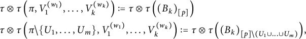 $$ \begin{align*} &\tau\otimes\tau\left(\pi,V_1^{(w_1)},\ldots,V_k^{(w_k)}\right):=\tau\otimes \tau\left(\left(B_{k}\right)_{[p]}\right)\\ &\tau\otimes\tau \left(\pi\setminus \{U_1,\ldots,U_{m}\},V_1^{(w_1)},\ldots,V_{k}^{(w_{k})}\right):=\tau\otimes \tau\left(\left(B_k\right)_{[p]\setminus \left(U_1\cup\ldots\cup U_{m}\right)}\right)\hspace{-1.5pt}, \end{align*} $$
where
 $U_1,\ldots ,U_{m},V_1,\ldots ,V_{k} \in \pi $
and
$U_1,\ldots ,U_{m},V_1,\ldots ,V_{k} \in \pi $
and
 $$ \begin{align*} B_{k}=B_k\left(V_1^{(w_1)},\dots,V_{k}^{(w_k)}\right)\hspace{-1.5pt}. \end{align*} $$
Note first that at each step k, the distribution of
 $(b_{i_{v_1},k},b_{i_{v_2},k})$
for a block
$(b_{i_{v_1},k},b_{i_{v_2},k})$
for a block
 $V=\{v_1<v_2\} \in \pi $
can be written as one of the following four cases.
$V=\{v_1<v_2\} \in \pi $
can be written as one of the following four cases.
-
(1) The blocks
$V_1,\ldots ,V_k$
do not cross V, and we have where we recall that
$$ \begin{align*} &b_{i_{v_1},k}=\frac{1}{\delta}\left(a_{i_{v_1}}\otimes a_{i_{v_1}}-\lambda^2\right)\hspace{-1.5pt};\\ &b_{i_{v_2},k}=\frac{1}{\delta}\left(a_{i_{v_1}}\otimes a_{i_{v_1}}-\lambda^2\right)\hspace{-1.5pt}, \end{align*} $$
$i_{v_1}=i_{v_2}$
.
-
(2) All blocks
$V_j$
that cross V have the same color
$w_j=0$
, and we have
$$ \begin{align*} &b_{i_{v_1},k}=\frac{1}{\delta}\left(\tilde{a}_{i_{v_1}}\otimes a_{i_{v_1}}-\lambda^2\right)\hspace{-1.5pt};\\ &b_{i_{v_2},k}=\frac{1}{\delta}\left(a_{i_{v_1}}\otimes a_{i_{v_1}}-\lambda^2\right)\hspace{-1.5pt}. \end{align*} $$
-
(3) All blocks
$V_j$
that cross V have the same color
$w_j=1$
, and we have
$$ \begin{align*} &b_{i_{v_1},k}=\frac{1}{\delta}\left(a_{i_{v_1}}\otimes \tilde{a}_{i_{v_1}}-\lambda^2\right)\hspace{-1.5pt};\\ &b_{i_{v_2},k}=\frac{1}{\delta}\left(a_{i_{v_1}}\otimes a_{i_{v_1}}-\lambda^2\right)\hspace{-1.5pt}. \end{align*} $$
-
(4) Otherwise, there exist two blocks
$V_{j_1},V_{j_2}$
that cross V such that
$w_{j_1}\ne w_{j_2}$
, that is, they have different colors, and then
$$ \begin{align*} &b_{i_{v_1},k}=\frac{1}{\delta}\left(\tilde{a}_{i_{v_1}}\otimes \tilde{a}_{i_{v_1}}-\lambda^2\right)\hspace{-1.5pt};\\ &b_{i_{v_2},k}=\frac{1}{\delta}\left(a_{i_{v_1}}\otimes a_{i_{v_1}}-\lambda^2\right)\hspace{-1.5pt}. \end{align*} $$


We remark that even if the choices of replacements do not always happen for
 $b_{i_{v_1}}$
, the joint distribution of
$b_{i_{v_1}}$
, the joint distribution of
 $(b_{i_{v_1},k},b_{i_{v_2},k})$
can always be written as one of those four cases since the variables are free identically distributed. For instance, we have
$(b_{i_{v_1},k},b_{i_{v_2},k})$
can always be written as one of those four cases since the variables are free identically distributed. For instance, we have
 $$ \begin{align*} (a\otimes a,a\otimes \tilde{a})\overset{d}{=}(a\otimes \tilde{a},a\otimes a)\overset{d}{=}(\tilde{a}\otimes a,\tilde{a}\otimes \tilde{a}), \end{align*} $$
and so on. Let
 $$ \begin{align*} &\theta \in \{0,1\}^4,\\ &\sum_{j \in [4]}\theta_j=1, \end{align*} $$
and denote
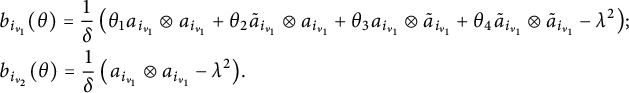 $$ \begin{align*} &b_{i_{v_1}}(\theta)=\frac{1}{\delta}\left(\theta_1 a_{i_{v_1}}\otimes a_{i_{v_1}}+\theta_2 \tilde{a}_{i_{v_1}}\otimes a_{i_{v_1}}+\theta_3 a_{i_{v_1}}\otimes \tilde{a}_{i_{v_1}}+\theta_4 \tilde{a}_{i_{v_1}}\otimes \tilde{a}_{i_{v_1}}-\lambda^2\right)\hspace{-1.5pt};\\ &b_{i_{v_2}}(\theta)=\frac{1}{\delta}\left(a_{i_{v_1}}\otimes a_{i_{v_1}}-\lambda^2\right)\hspace{-1.5pt}. \end{align*} $$
The choice of
 $\theta :=\theta \left (V, V_1^{(w_1)}\ldots , V_k^{(w_k)}\right )$
corresponds to the case in which we are, that is, we define
$\theta :=\theta \left (V, V_1^{(w_1)}\ldots , V_k^{(w_k)}\right )$
corresponds to the case in which we are, that is, we define
 $\theta $
as the binary vector such that
$\theta $
as the binary vector such that
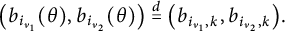 $$ \begin{align*} \left(b_{i_{v_1}}(\theta),b_{i_{v_2}}(\theta)\right)\overset{d}{=}\left(b_{i_{v_1},k},b_{i_{v_2},k}\right)\hspace{-1.5pt}. \end{align*} $$
Let
 $V=\{v_1<v_2\} \in \pi \setminus \{V_1,\ldots , V_k\}$
and
$V=\{v_1<v_2\} \in \pi \setminus \{V_1,\ldots , V_k\}$
and
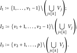 $$ \begin{align*} &I_1:=\{1,\ldots,v_1-1\}\setminus \left(\bigcup_{j \in [k]}V_j\right)\hspace{-1.5pt};\\ &I_2:=\{v_1+1,\ldots,v_2-1\}\setminus \left(\bigcup_{j \in [k]}V_j\right)\hspace{-1.5pt};\\ &I_3:=\{v_2+1,\ldots,p\}\setminus \left(\bigcup_{j \in [k]}V_j\right)\hspace{-1.5pt}. \end{align*} $$
Our first goal is to obtain the contribution and coloring of V to
 $$ \begin{align*} \tau\otimes\tau \left(\pi\setminus \{V_1,\ldots,V_{k}\},V_1^{(w_1)},\ldots,V_{k}^{(w_{k})}\right)=\tau\otimes \tau\left(\left(B_k\right)_{I_1}b_{i_{v_1},k}\left(B_k\right)_{I_2}b_{i_{v_2},k}\left(B_k\right)_{I_3}\right)\hspace{-1.5pt}, \end{align*} $$
according to the value of
 $\theta = \theta \left (V, V_1^{(w_1)}\ldots , V_k^{(w_k)}\right )\in \{0,1\}^4$
, where
$\theta = \theta \left (V, V_1^{(w_1)}\ldots , V_k^{(w_k)}\right )\in \{0,1\}^4$
, where
 $$ \begin{align*} B_k=B_k\left(V_1^{(w_1)},\ldots,V_k^{(w_k)}\right)\hspace{-1.5pt}. \end{align*} $$
We recall that
 $$ \begin{align*} \tau\otimes\tau\left(\left(B_k\right)_{I_1}\left(B_k\right)_{I_2}\left(B_k\right)_{I_3}\right)&=\tau\otimes \tau\left(\left(B_k\right)_{[p]\setminus \left(V_1\cup \ldots \cup V_k \cup V\right)}\right)\\ &=\tau\otimes \tau\left(\pi\setminus\{V_1,\ldots,V_k,V\},V_1^{(w_1)},\ldots,V_k^{(w_k)}\right) \end{align*} $$
To simplify the notation, we denote
 $$ \begin{align} h:=|I_1|+|I_2|+|I_3|=p-2(k+1). \end{align} $$
We divide the four cases into the next four lemmas.
Lemma 5.5 (Case
$\theta _1=1$
)

Let
 $p \ge 4$
be an even integer,
$p \ge 4$
be an even integer,
 $\pi \in P_2^{\operatorname {con}}(p)$
. Let
$\pi \in P_2^{\operatorname {con}}(p)$
. Let
 $V_1,\ldots ,V_k \in \pi $
be blocks,
$V_1,\ldots ,V_k \in \pi $
be blocks,
 $w \in \{0,1\}^k$
be a coloring of
$w \in \{0,1\}^k$
be a coloring of
 $V_1,\ldots ,V_k$
and
$V_1,\ldots ,V_k$
and
 $$ \begin{align*} B_k=B_k\left(V_1^{(w_1)},\ldots,V_k^{(w_k)}\right)=\left(b_{i_j,k}\right)_{j \in [p]}. \end{align*} $$
Let
 $V=\{v_1<v_2\} \in \pi \setminus \{V_1,\ldots ,V_{k}\}$
and the joint law
$V=\{v_1<v_2\} \in \pi \setminus \{V_1,\ldots ,V_{k}\}$
and the joint law
 $$ \begin{align*} \left(b_{i_{v_1},k},b_{i_{v_2},k}\right)\overset{d}{=}\left(b_{i_{v_1}}(\theta),b_{i_{v_2}}(\theta)\right)\hspace{-1.5pt}. \end{align*} $$
If
 $\theta _1=1$
, we have
$\theta _1=1$
, we have
 $$ \begin{align*} &\tau\otimes\tau \left(\pi\setminus \{V_1,\ldots,V_{k}\},V_1^{(w_1)},\ldots,V_{k}^{(w_{k})}\right)\\ &=\frac{q}{2}\sum_{w=0,1}\tau\otimes\tau \left(\pi\setminus \{V_1,\ldots,V_k,V\},V_1^{(w_1)},\ldots,V_{k}^{(w_{k})},V^{(w)}\right)\hspace{-1.5pt}. \end{align*} $$
Proof To simplify the notation, let
 $$ \begin{align*} T:=\tau\otimes\tau \left(\pi\setminus \{V_1,\ldots,V_{k}\},V_1^{(w_1)},\ldots,V_{k}^{(w_{k})}\right)\hspace{-1.5pt}. \end{align*} $$
Then, we must prove that
 $$ \begin{align*} T=\frac{q}{2}\sum_{w=0,1}\tau\otimes\tau \left(\pi\setminus \{V_1,\ldots,V_k,V\},V_1^{(w_1)},\ldots,V_{k}^{(w_{k})},V^{(w)}\right)\hspace{-1.5pt}. \end{align*} $$
As
 $\theta _1=1$
, we can write
$\theta _1=1$
, we can write
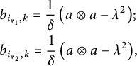 $$ \begin{align*} &b_{i_{v_1},k}=\frac{1}{\delta}\left(a\otimes a-\lambda^2\right)\hspace{-1.5pt};\\ &b_{i_{v_2},k}=\frac{1}{\delta}\left(a\otimes a-\lambda^2\right)\hspace{-1.5pt}, \end{align*} $$
where
 $a:=a_{i_{v_1}}$
. We get by Lemma 4.1 that
$a:=a_{i_{v_1}}$
. We get by Lemma 4.1 that
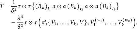 $$ \begin{align} T&=\frac{1}{\delta^2}\tau\otimes \tau\left\{\left(B_k\right)_{I_1}a\otimes a\left(B_k\right)_{I_2}a\otimes a\left(B_k\right)_{I_3}\right\}\nonumber\\ & \quad -\frac{\lambda^4}{\delta^2}\tau\otimes \tau\left(\pi\setminus\{V_1,\ldots,V_k,V\},V_1^{(w_1)},\ldots,V_k^{(w_k)}\right)\hspace{-1.5pt}. \end{align} $$
Let us write
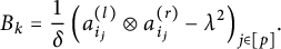 $$ \begin{align*} B_k=\frac{1}{\delta}\left(a_{i_j}^{(l)}\otimes a_{i_j}^{(r)}-\lambda^2\right)_{j \in [p]}\hspace{-1.5pt}. \end{align*} $$
Then
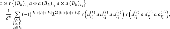 $$ \begin{align*} &\tau\otimes \tau\left\{\left(B_k\right)_{I_1}a\otimes a\left(B_k\right)_{I_2}a\otimes a\left(B_k\right)_{I_3}\right\}\\ &=\frac{1}{\delta^{h}}\sum_{\substack{J_1 \subseteq I_1\\ J_2 \subseteq I_2\\ J_3 \subseteq I_3}}(-1)^{|J_1|+|J_2|+|J_3|}\lambda^{2(|J_1|+|J_2|+|J_3|)}\tau\left(a_{J_1^c}^{(l)}\, a \, a_{J_2^c}^{(l)}\, a \, a_{J_3^c}^{(l)}\right)\tau\left(a_{J_1^c}^{(r)}\, a \, a_{J_2^c}^{(r)}\, a\, a_{J_3^c}^{(r)}\right)\hspace{-1.5pt}, \end{align*} $$
where h is defined as in (12). We use Lemma 2.1 and compute
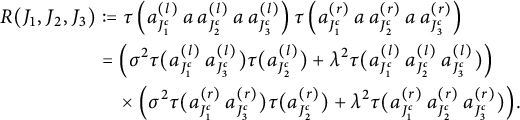 $$ \begin{align*} R(J_1,J_2,J_3) &:=\tau\left(a_{J_1^c}^{(l)}\, a \, a_{J_2^c}^{(l)}\, a \, a_{J_3^c}^{(l)}\right)\tau\left(a_{J_1^c}^{(r)}\, a \, a_{J_2^c}^{(r)}\, a\, a_{J_3^c}^{(r)}\right)\\ &=\left(\sigma^2\tau(a_{J_1^c}^{(l)}\, a_{J_3^c}^{(l)})\tau(a_{J_2^c}^{(l)})+\lambda^2\tau(a_{J_1^c}^{(l)}\, a_{J_2^c}^{(l)}\, a_{J_3^c}^{(l)})\right) \\ & \quad \times \left(\sigma^2\tau(a_{J_1^c}^{(r)}\, a_{J_3^c}^{(r)})\tau(a_{J_2^c}^{(r)})+\lambda^2\tau(a_{J_1^c}^{(r)}\, a_{J_2^c}^{(r)}\, a_{J_3^c}^{(r)})\right)\hspace{-1.5pt}. \end{align*} $$
After the expansion, we have
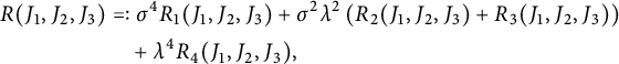 $$ \begin{align*} R(J_1,J_2,J_3) & =:\sigma^4R_1(J_1,J_2,J_3)+\sigma^2\lambda^2 \left(R_2(J_1,J_2,J_3)+R_3(J_1,J_2,J_3)\right) \\ &\quad +\lambda^4R_4(J_1,J_2,J_3), \end{align*} $$
where we choose
 $R_2$
to be the term with factor
$R_2$
to be the term with factor
 $\tau (a_{J_1^c}^{(l)}\, a_{J_2^c}^{(l)}\, a_{J_3^c}^{(l)})$
. For
$\tau (a_{J_1^c}^{(l)}\, a_{J_2^c}^{(l)}\, a_{J_3^c}^{(l)})$
. For
 $R_1$
, we have
$R_1$
, we have
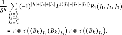 $$ \begin{align*} &\frac{1}{\delta^h}\sum_{\substack{J_1 \subseteq I_1\\ J_2 \subseteq I_2\\ J_3 \subseteq I_3}}(-1)^{|J_1|+|J_2|+|J_3|}\lambda^{2(|J_1|+|J_2|+|J_3|)}R_1(J_1,J_2,J_3)\\ &\quad =\tau\otimes \tau \left(\left(B_k\right)_{I_1}\left(B_k\right)_{I_3}\right)\tau\otimes \tau\left(\left(B_k\right)_{I_2}\right)\hspace{-1.5pt}. \end{align*} $$
Since
 $\pi $
is connected, V crosses at least one block
$\pi $
is connected, V crosses at least one block
 $U=\{j,j'\} \in \pi $
. Therefore, we assume
$U=\{j,j'\} \in \pi $
. Therefore, we assume
 $j \in I_2$
whose matching symbol
$j \in I_2$
whose matching symbol
 $j' \in I_1\cup I_3$
. By Lemma 4.1, we have
$j' \in I_1\cup I_3$
. By Lemma 4.1, we have
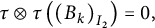 $$ \begin{align*} \tau\otimes \tau\left(\left(B_k\right)_{I_2}\right)=0, \end{align*} $$
and the contribution of
 $R_1$
is zero. For
$R_1$
is zero. For
 $R_4$
, we have
$R_4$
, we have
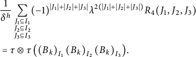 $$ \begin{align*} &\frac{1}{\delta^h}\sum_{\substack{J_1 \subseteq I_1\\ J_2 \subseteq I_2\\ J_3 \subseteq I_3}}(-1)^{|J_1|+|J_2|+|J_3|}\lambda^{2(|J_1|+|J_2|+|J_3|)}R_4(J_1,J_2,J_3)\\ &=\tau\otimes \tau \left(\left(B_k\right)_{I_1}\left(B_k\right)_{I_2}\left(B_k\right)_{I_3}\right)\hspace{-1.5pt}. \end{align*} $$
Since
 $$ \begin{align*} \tau\otimes \tau \left(\left(B_k\right)_{I_1}\left(B_k\right)_{I_2}\left(B_k\right)_{I_3}\right)=\tau\otimes\tau\left(\pi\setminus\{V_1,\ldots,V_k,V\},V_1^{(w_1)},\ldots,V_k^{(w_k)}\right)\hspace{-1.5pt}, \end{align*} $$
its contribution cancels out with
 $\frac {\lambda ^4}{\delta ^2}\tau \otimes \tau \left (\pi \setminus \{V_1,\ldots ,V_k,V\},V_1^{(w_1)},\ldots ,V_k^{(w_k)}\right )$
in (13). For
$\frac {\lambda ^4}{\delta ^2}\tau \otimes \tau \left (\pi \setminus \{V_1,\ldots ,V_k,V\},V_1^{(w_1)},\ldots ,V_k^{(w_k)}\right )$
in (13). For
 $R_2$
, let us first denote by
$R_2$
, let us first denote by
 $\left (\overline {a}_{i_j}^{(l)},\overline {a}_{i_j}^{(r)}\right )_{j\in [p]}$
the variables in
$\left (\overline {a}_{i_j}^{(l)},\overline {a}_{i_j}^{(r)}\right )_{j\in [p]}$
the variables in
 $B_{k+1}\left (V_1^{(w_1)},\ldots ,V_{k}^{(w_k)},V^{(1)}\right )$
, namely,
$B_{k+1}\left (V_1^{(w_1)},\ldots ,V_{k}^{(w_k)},V^{(1)}\right )$
, namely,
 $$ \begin{align*} B_{k+1}=B_{k+1}\left(V_1^{(w_1)},\ldots,V_{k}^{(w_k)},V^{(1)}\right)=\frac{1}{\delta}\left(\overline{a}_{i_j}^{(l)}\otimes \overline{a}_{i_j}^{(r)}-\lambda^2\right)_{j \in [p]}. \end{align*} $$
We then have
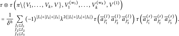 $$ \begin{align*} &\tau\otimes\tau\left(\pi\setminus\{V_1,\ldots,V_k,V\},V_1^{(w_1)},\ldots,V_{k}^{(w_k)},V^{(1)}\right)\\ &=\frac{1}{\delta^h}\sum_{\substack{J_1 \subseteq I_1\\ J_2 \subseteq I_2\\ J_3 \subseteq I_3}}(-1)^{|J_1|+|J_2|+|J_3|}\lambda^{2(|J_1|+|J_2|+|J_3|)}\tau\left(\overline{a}_{J_1^c}^{(l)}\, \overline{a}_{J_2^c}^{(l)}\, \overline{a}_{J_3^c}^{(l)}\right)\tau\left(\overline{a}_{J_1^c}^{(r)}\, \overline{a}_{J_2^c}^{(r)}\, \overline{a}_{J_3^c}^{(r)}\right)\hspace{-1.5pt}. \end{align*} $$
By definition, the color
 $w_{k+1}=1$
does not affect the left legs, hence
$w_{k+1}=1$
does not affect the left legs, hence
 $$ \begin{align*} \overline{a}_{i_j}^{(l)}=a_{i_j}^{(l)}. \end{align*} $$
For the right legs and a block
 $U=\{t_1<t_2\}$
, let us divide it into two cases.
$U=\{t_1<t_2\}$
, let us divide it into two cases.
-
(1) If U does not cross V, we have
$$ \begin{align*} &\overline{a}_{i_{t_1}}^{(r)}=a_{i_{t_1}}^{(r)};\\ &\overline{a}_{i_{t_2}}^{(r)}=a_{i_{t_2}}^{(r)}. \end{align*} $$
-
(2) Otherwise, either
$t_1 \in I_2$
and
$t_2 \in I_1\cup I_3$
or
$t_1 \in I_1 \cup I_3$
and
$t_2 \in I_2$
. By the definition of the color
$w_{k+1}=1$
, we have
$$ \begin{align*} &\overline{a}_{i_{t_1}}^{(r)}=\tilde{a}_{i_{t_1}};\\ &\overline{a}_{i_{t_2}}^{(r)}=a_{i_{t_1}}. \end{align*} $$


Since
 $(a_k)_{k \in \mathbb {N}}$
and
$(a_k)_{k \in \mathbb {N}}$
and
 $(\tilde {a}_k)_{k \in \mathbb {N}}$
are free copies of a, the following holds. First, let
$(\tilde {a}_k)_{k \in \mathbb {N}}$
are free copies of a, the following holds. First, let
 $t \in I_2$
. Consider
$t \in I_2$
. Consider
 $t'$
its matching symbol, that is,
$t'$
its matching symbol, that is,
 $\{t,t'\} \in \pi $
and
$\{t,t'\} \in \pi $
and
 $i_t=i_{t'} \ne i_j$
, for all
$i_t=i_{t'} \ne i_j$
, for all
 $j \notin \{t,t'\}$
. Recall that, by the definition in (11), we have
$j \notin \{t,t'\}$
. Recall that, by the definition in (11), we have
 $$ \begin{align*} \overline{a}_{i_t}^{(r)},\overline{a}_{i_{t'}}^{(r)} \in \{a_{i_t},\tilde{a}_{i_t}\}. \end{align*} $$
If
 $t' \in I_2$
, Case (1) implies that the law of
$t' \in I_2$
, Case (1) implies that the law of
 $(\overline {a}_{i_t}^{(r)},\overline {a}_{i_{t'}}^{(r)})$
is equal to the law of
$(\overline {a}_{i_t}^{(r)},\overline {a}_{i_{t'}}^{(r)})$
is equal to the law of
 $({a}_{i_t}^{(r)},{a}_{i_{t'}}^{(r)})$
. If
$({a}_{i_t}^{(r)},{a}_{i_{t'}}^{(r)})$
. If
 $t' \in I_1\cup I_3$
, as
$t' \in I_1\cup I_3$
, as
 $a_{i_t},\tilde {a}_{i_t}$
are free identically distributed and free from
$a_{i_t},\tilde {a}_{i_t}$
are free identically distributed and free from
 $(a_k)_{k \ne i_t},(\tilde {a}_k)_{k \ne i_t}$
, we have
$(a_k)_{k \ne i_t},(\tilde {a}_k)_{k \ne i_t}$
, we have
 $$ \begin{align} \left((\overline{a}_{i_j}^{(r)})_{j \in I_2\setminus\{t\}},\overline{a}_{i_t}^{(r)}\right)\overset{d}{=}\left((\overline{a}^{(r)}_{i_j})_{j \in I_2\setminus\{t\}},a_{i_t}\right)\overset{d}{=}\left((\overline{a}^{(r)}_{i_j})_{j \in I_2\setminus\{t\}},a_{i_t}^{(r)}\right)\hspace{-1.5pt}. \end{align} $$
Applying the above equalities in distribution for all
 $t \in I_2$
, namely, Case (1) for
$t \in I_2$
, namely, Case (1) for
 $t' \in I_2$
and (14) for
$t' \in I_2$
and (14) for
 $t' \notin I_2$
, we get
$t' \notin I_2$
, we get
 $$ \begin{align*} \left(\overline{a}_{i_j}^{(r)}\right)_{j \in I_2}\overset{d}{=}\left(a_{i_j}^{(r)}\right)_{j \in I_2}. \end{align*} $$
By symmetry, we also have
 $$ \begin{align*} \left(\overline{a}_{i_j}^{(r)}\right)_{j \in I_1\cup I_3}\overset{d}{=}\left(a_{i_j}^{(r)}\right)_{j \in I_1\cup I_3}. \end{align*} $$
Additionally,
 $\left (\overline {a}_{i_j}^{(r)}\right )_{j \in I_2}$
is now free from
$\left (\overline {a}_{i_j}^{(r)}\right )_{j \in I_2}$
is now free from
 $\left (\overline {a}_{i_j}^{(r)}\right )_{j \in I_1\cup I_3}$
. Indeed, let us show that each variable
$\left (\overline {a}_{i_j}^{(r)}\right )_{j \in I_1\cup I_3}$
. Indeed, let us show that each variable
 $\overline {a}_{i_t}^{(r)}$
is free from
$\overline {a}_{i_t}^{(r)}$
is free from
 $\left (\overline {a}_{i_j}^{(r)}\right )_{j \in I_1\cup I_3}$
, for all
$\left (\overline {a}_{i_j}^{(r)}\right )_{j \in I_1\cup I_3}$
, for all
 $t \in I_2$
. Consider
$t \in I_2$
. Consider
 $t'$
its matching symbol. First, if
$t'$
its matching symbol. First, if
 $t' \in I_2$
, the fact that
$t' \in I_2$
, the fact that
 $(a_k)_{k \in \mathbb {N}}$
and
$(a_k)_{k \in \mathbb {N}}$
and
 $(\tilde {a}_k)_{k \in \mathbb {N}}$
are free identically distributed collections implies that
$(\tilde {a}_k)_{k \in \mathbb {N}}$
are free identically distributed collections implies that
 $\overline {a}_{i_t}^{(r)}$
(and
$\overline {a}_{i_t}^{(r)}$
(and
 $\overline {a}_{i_{t'}}^{(r)}$
) is free from
$\overline {a}_{i_{t'}}^{(r)}$
) is free from
 $\left (\overline {a}_{i_j}^{(r)}\right )_{j \in I_1\cup I_3}$
. If
$\left (\overline {a}_{i_j}^{(r)}\right )_{j \in I_1\cup I_3}$
. If
 $t' \in I_1\cup I_3$
, Case (2) implies that
$t' \in I_1\cup I_3$
, Case (2) implies that
 $\overline {a}_{i_t}^{(r)}$
is free from
$\overline {a}_{i_t}^{(r)}$
is free from
 $\overline {a}_{i_{t'}}^{(r)}$
and then again
$\overline {a}_{i_{t'}}^{(r)}$
and then again
 $\overline {a}_{i_t}^{(r)}$
is free from
$\overline {a}_{i_t}^{(r)}$
is free from
 $\left (\overline {a}_{i_j}^{(r)}\right )_{j \in I_1\cup I_3}$
.
$\left (\overline {a}_{i_j}^{(r)}\right )_{j \in I_1\cup I_3}$
.
In summary, by freeness, we have
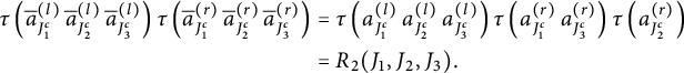 $$ \begin{align*} \tau\left(\overline{a}_{J_1^c}^{(l)}\, \overline{a}_{J_2^c}^{(l)}\, \overline{a}_{J_3^c}^{(l)}\right)\tau\left(\overline{a}_{J_1^c}^{(r)}\, \overline{a}_{J_2^c}^{(r)}\, \overline{a}_{J_3^c}^{(r)}\right)&=\tau\left(a_{J_1^c}^{(l)}\, a_{J_2^c}^{(l)}\, a_{J_3^c}^{(l)}\right)\tau\left(a_{J_1^c}^{(r)}\, a_{J_3^c}^{(r)}\right)\tau\left(a_{J_2^c}^{(r)}\right)\\ &=R_2(J_1,J_2,J_3). \end{align*} $$
Therefore
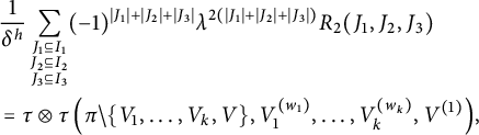 $$ \begin{align*} &\frac{1}{\delta^h}\sum_{\substack{J_1 \subseteq I_1\\ J_2 \subseteq I_2\\ J_3 \subseteq I_3}}(-1)^{|J_1|+|J_2|+|J_3|}\lambda^{2(|J_1|+|J_2|+|J_3|)}R_2(J_1,J_2,J_3)\\ &=\tau\otimes \tau\left(\pi\setminus\{V_1,\ldots,V_k,V\},V_1^{(w_1)},\ldots,V_k^{(w_k)},V^{(1)}\right)\hspace{-1.5pt}, \end{align*} $$
Following the same reasoning, it follows that
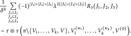 $$ \begin{align*} &\frac{1}{\delta^h}\sum_{\substack{J_1 \subseteq I_1\\ J_2 \subseteq I_2\\ J_3 \subseteq I_3}}(-1)^{|J_1|+|J_2|+|J_3|}\lambda^{2(|J_1|+|J_2|+|J_3|)}R_3(J_1,J_2,J_3)\\ &=\tau\otimes \tau\left(\pi\setminus\{V_1,\ldots,V_k,V\},V_1^{(w_1)},\ldots,V_k^{(w_k)},V^{(0)}\right)\hspace{-1.5pt}. \end{align*} $$
Combining the above relations in T, we get
 $$ \begin{align*} T=\frac{\sigma^2\lambda^2}{\delta^2}\sum_{w=0,1}\tau\otimes \tau\left(\pi\setminus\{V_1,\ldots,V_k,V\},V_1^{(w_1)},\ldots,V_k^{(w_k)},V^{(w)}\right)\hspace{-1.5pt}. \end{align*} $$
It remains to note that
 $$ \begin{align*} \frac{\sigma^2\lambda^2}{\delta^2}=\frac{q}{2}, \end{align*} $$
to finish the proof.
Lemma 5.6 (Case
$\theta _2=1$
)

Let
 $p \ge 4$
be an even integer,
$p \ge 4$
be an even integer,
 $\pi \in P_2^{\operatorname {con}}(p)$
. Let
$\pi \in P_2^{\operatorname {con}}(p)$
. Let
 $V_1,\ldots ,V_k \in \pi $
be blocks,
$V_1,\ldots ,V_k \in \pi $
be blocks,
 $w \in \{0,1\}^k$
be a coloring of
$w \in \{0,1\}^k$
be a coloring of
 $V_1,\ldots ,V_k$
and
$V_1,\ldots ,V_k$
and
 $$ \begin{align*} B_k=B_k\left(V_1^{(w_1)},\ldots,V_k^{(w_k)}\right)=\left(b_{i_j,k}\right)_{j \in [p]}. \end{align*} $$
Let
 $V=\{v_1<v_2\} \in \pi \setminus \{V_1,\ldots ,V_{k}\}$
and the joint law
$V=\{v_1<v_2\} \in \pi \setminus \{V_1,\ldots ,V_{k}\}$
and the joint law
 $$ \begin{align*} \left(b_{i_{v_1},k},b_{i_{v_2},k}\right)\overset{d}{=}\left(b_{i_{v_1}}(\theta),b_{i_{v_2}}(\theta)\right)\hspace{-1.5pt}. \end{align*} $$
If
 $\theta _2=1$
, we have
$\theta _2=1$
, we have
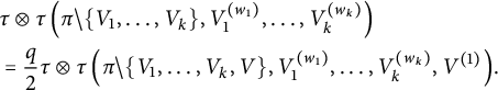 $$ \begin{align*} &\tau\otimes\tau \left(\pi\setminus \{V_1,\ldots,V_{k}\},V_1^{(w_1)},\ldots,V_{k}^{(w_{k})}\right)\\ &=\frac{q}{2}\tau\otimes\tau \left(\pi\setminus \{V_1,\ldots,V_{k},V\},V_1^{(w_1)},\ldots,V_{k}^{(w_{k})},V^{(1)}\right)\hspace{-1.5pt}. \end{align*} $$
Proof We must prove that
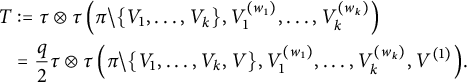 $$ \begin{align*} T&:=\tau\otimes\tau \left(\pi\setminus \{V_1,\ldots,V_{k}\},V_1^{(w_1)},\ldots,V_{k}^{(w_{k})}\right)\\ &=\frac{q}{2}\tau\otimes\tau \left(\pi\setminus \{V_1,\ldots,V_{k},V\},V_1^{(w_1)},\ldots,V_{k}^{(w_{k})},V^{(1)}\right)\hspace{-1.5pt}. \end{align*} $$
As
 $\theta _2=1$
, we can write
$\theta _2=1$
, we can write
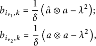 $$ \begin{align*} &b_{i_{v_1},k}=\frac{1}{\delta}\left(\tilde{a}\otimes a-\lambda^2\right)\hspace{-1.5pt};\\ &b_{i_{v_2},k}=\frac{1}{\delta}\left(a\otimes a-\lambda^2\right)\hspace{-1.5pt}, \end{align*} $$
where
 $a:=a_{i_{v_1}}$
. We have
$a:=a_{i_{v_1}}$
. We have
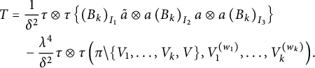 $$ \begin{align} T&=\frac{1}{\delta^2}\tau\otimes \tau\left\{\left(B_k\right)_{I_1}\tilde{a}\otimes a\left(B_k\right)_{I_2}a\otimes a\left(B_k\right)_{I_3}\right\}\nonumber \\ &\quad -\frac{\lambda^4}{\delta^2}\tau\otimes \tau\left(\pi\setminus\{V_1,\ldots,V_k,V\},V_1^{(w_1)},\ldots,V_k^{(w_k)}\right)\hspace{-1.5pt}. \end{align} $$
We write again
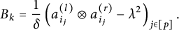 $$ \begin{align*} B_k=\frac{1}{\delta}\left(a_{i_j}^{(l)}\otimes a_{i_j}^{(r)}-\lambda^2\right)_{j \in [p]}. \end{align*} $$
Then
 $$ \begin{align*} &\tau\otimes \tau\left\{\left(B_k\right)_{I_1}\tilde{a}\otimes a\left(B_k\right)_{I_2}a\otimes a\left(B_k\right)_{I_3}\right\}\\ &=\frac{1}{\delta^h}\sum_{\substack{J_1 \subseteq I_1\\ J_2 \subseteq I_2\\ J_3 \subseteq I_3}}(-1)^{|J_1|+|J_2|+|J_3|}\lambda^{2(|J_1|+|J_2|+|J_3|)}\tau\left(a_{J_1^c}^{(l)}\, \tilde{a} \, a_{J_2^c}^{(l)}\, a \, a_{J_3^c}^{(l)}\right)\tau\left(a_{J_1^c}^{(r)}\, a \, a_{J_2^c}^{(r)}\, a\, a_{J_3^c}^{(r)}\right)\hspace{-1.5pt}, \end{align*} $$
where h is defined in (12). We use Lemmas 2.1 and 4.1 to compute
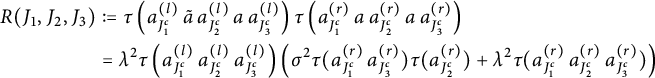 $$ \begin{align*} R(J_1,J_2,J_3)&:=\tau\left(a_{J_1^c}^{(l)}\, \tilde{a} \, a_{J_2^c}^{(l)}\, a \, a_{J_3^c}^{(l)}\right)\tau\left(a_{J_1^c}^{(r)}\, a \, a_{J_2^c}^{(r)}\, a\, a_{J_3^c}^{(r)}\right)\\ &=\lambda^2\tau\left(a_{J_1^c}^{(l)}\, a_{J_2^c}^{(l)}\, a_{J_3^c}^{(l)}\right)\left(\sigma^2\tau(a_{J_1^c}^{(r)}\, a_{J_3^c}^{(r)})\tau(a_{J_2^c}^{(r)})+\lambda^2\tau(a_{J_1^c}^{(r)}\, a_{J_2^c}^{(r)}\, a_{J_3^c}^{(r)})\right) \end{align*} $$
Hence
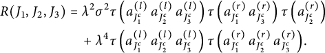 $$ \begin{align*} R(J_1,J_2,J_3)&=\lambda^2\sigma^2\tau\left(a_{J_1^c}^{(l)}\, a_{J_2^c}^{(l)}\, a_{J_3^c}^{(l)}\right)\tau\left(a_{J_1^c}^{(r)}\, a_{J_3^c}^{(r)}\right)\tau\left(a_{J_2^c}^{(r)}\right) \\ &\quad+\lambda^4\tau\left(a_{J_1^c}^{(l)}\, a_{J_2^c}^{(l)}\, a_{J_3^c}^{(l)}\right)\tau\left(a_{J_1^c}^{(r)}\, a_{J_2^c}^{(r)}\, a_{J_3^c}^{(r)}\right)\hspace{-1.5pt}. \end{align*} $$
Both terms already appeared in the proof of Lemma 5.5. The second term cancels out with
 $\frac {\lambda ^4}{\delta ^2}\tau \otimes \tau \left (\pi \setminus \{V_1,\ldots , V_k,V\}, V_1^{(w_1)},\ldots , V_k^{(w_k)}\right )$
in (15), and the contribution of the first is equal to
$\frac {\lambda ^4}{\delta ^2}\tau \otimes \tau \left (\pi \setminus \{V_1,\ldots , V_k,V\}, V_1^{(w_1)},\ldots , V_k^{(w_k)}\right )$
in (15), and the contribution of the first is equal to
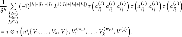 $$ \begin{align*} &\frac{1}{\delta^h}\sum_{\substack{J_1 \subseteq I_1\\ J_2 \subseteq I_2\\ J_3 \subseteq I_3}}(-1)^{|J_1|+|J_2|+|J_3|}\lambda^{2(|J_1|+|J_2|+|J_3|)}\tau\left(a_{J_1^c}^{(l)}\, a_{J_2^c}^{(l)}\, a_{J_3^c}^{(l)}\right)\tau\left(a_{J_1^c}^{(r)}\, a_{J_3^c}^{(r)}\right)\tau\left(a_{J_2^c}^{(r)}\right)\\ &=\tau\otimes \tau\left(\pi\setminus\{V_1,\ldots,V_k,V\},V_1^{(w_1)},\ldots,V_k^{(w_k)},V^{(1)}\right)\hspace{-1.5pt}. \end{align*} $$
We then have
 $$ \begin{align*} T=\frac{\sigma^2\lambda^2}{\delta^2}\tau\otimes \tau\left(\pi\setminus\{V_1,\ldots,V_k,V\},V_1^{(w_1)},\ldots,V_k^{(w_k)},V^{(1)}\right)\hspace{-1.5pt}, \end{align*} $$
and the result follows by the definition of q.
The case
 $\theta _3=1$
is symmetric to the case
$\theta _3=1$
is symmetric to the case
 $\theta _2=1$
in Lemma 5.6, and we omit the proof.
$\theta _2=1$
in Lemma 5.6, and we omit the proof.
Lemma 5.7 (Case
$\theta _3=1$
)

Let
 $p \ge 4$
be an even integer,
$p \ge 4$
be an even integer,
 $\pi \in P_2^{\operatorname {con}}(p)$
. Let
$\pi \in P_2^{\operatorname {con}}(p)$
. Let
 $V_1,\ldots ,V_k \in \pi $
be blocks,
$V_1,\ldots ,V_k \in \pi $
be blocks,
 $w \in \{0,1\}^k$
be a coloring of
$w \in \{0,1\}^k$
be a coloring of
 $V_1,\ldots ,V_k$
and
$V_1,\ldots ,V_k$
and
 $$ \begin{align*} B_k=B_k\left(V_1^{(w_1)},\ldots,V_k^{(w_k)}\right)=\left(b_{i_j,k}\right)_{j \in [p]}. \end{align*} $$
Let
 $V=\{v_1<v_2\} \in \pi \setminus \{V_1,\ldots ,V_{k}\}$
and the joint law
$V=\{v_1<v_2\} \in \pi \setminus \{V_1,\ldots ,V_{k}\}$
and the joint law
 $$ \begin{align*} \left(b_{i_{v_1},k},b_{i_{v_2},k}\right)\overset{d}{=}\left(b_{i_{v_1}}(\theta),b_{i_{v_2}}(\theta)\right)\hspace{-1.5pt}. \end{align*} $$
If
 $\theta _3=1$
, we have
$\theta _3=1$
, we have
 $$ \begin{align*} &\tau\otimes\tau \left(\pi\setminus \{V_1,\ldots,V_{k}\},V_1^{(w_1)},\ldots,V_{k}^{(w_{k})}\right)\\ &=\frac{q}{2}\tau\otimes\tau \left(\pi\setminus \{V_1,\ldots,V_{k},V\},V_1^{(w_1)},\ldots,V_{k}^{(w_{k})},V^{(0)}\right)\hspace{-1.5pt}. \end{align*} $$
Finally, the case
 $\theta _4=1$
has a null contribution.
$\theta _4=1$
has a null contribution.
Lemma 5.8 (Case
$\theta _4=1$
)

Let
 $p \ge 4$
be an even integer,
$p \ge 4$
be an even integer,
 $\pi \in P_2^{\operatorname {con}}(p)$
. Let
$\pi \in P_2^{\operatorname {con}}(p)$
. Let
 $V_1,\ldots ,V_k \in \pi $
be blocks,
$V_1,\ldots ,V_k \in \pi $
be blocks,
 $w \in \{0,1\}^k$
be a coloring of
$w \in \{0,1\}^k$
be a coloring of
 $V_1,\ldots ,V_k$
and
$V_1,\ldots ,V_k$
and
 $$ \begin{align*} B_k=B_k\left(V_1^{(w_1)},\ldots,V_k^{(w_k)}\right)=\left(b_{i_j,k}\right)_{j \in [p]}. \end{align*} $$
Let
 $V=\{v_1<v_2\} \in \pi \setminus \{V_1,\ldots ,V_{k}\}$
and the joint law
$V=\{v_1<v_2\} \in \pi \setminus \{V_1,\ldots ,V_{k}\}$
and the joint law
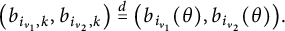 $$ \begin{align*} \left(b_{i_{v_1},k},b_{i_{v_2},k}\right)\overset{d}{=}\left(b_{i_{v_1}}(\theta),b_{i_{v_2}}(\theta)\right)\hspace{-1.5pt}. \end{align*} $$
If
 $\theta _4=1$
, we have
$\theta _4=1$
, we have
 $$ \begin{align*} &\tau\otimes\tau \left(\pi\setminus \{V_1,\ldots,V_{k}\},V_1^{(w_1)},\ldots,V_{k}^{(w_{k})}\right)=0. \end{align*} $$
Proof Similarly to the previous proofs, we must show that
 $$ \begin{align*} T:=\tau\otimes\tau \left(\pi\setminus \{V_1,\ldots,V_{k}\},V_1^{(w_1)},\ldots,V_{k}^{(w_{k})}\right) =0. \end{align*} $$
As
 $\theta _4=1$
, we can write
$\theta _4=1$
, we can write
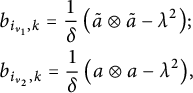 $$ \begin{align*} &b_{i_{v_1},k}=\frac{1}{\delta}\left(\tilde{a}\otimes \tilde{a}-\lambda^2\right)\hspace{-1.5pt};\\ &b_{i_{v_2},k}=\frac{1}{\delta}\left(a\otimes a-\lambda^2\right)\hspace{-1.5pt}, \end{align*} $$
where
 $a:=a_{i_{v_1}}$
. First note that
$a:=a_{i_{v_1}}$
. First note that
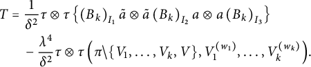 $$ \begin{align*} T&=\frac{1}{\delta^2}\tau\otimes \tau\left\{\left(B_k\right)_{I_1}\tilde{a}\otimes \tilde{a}\left(B_k\right)_{I_2}a\otimes a\left(B_k\right)_{I_3}\right\}\\ &\quad-\frac{\lambda^4}{\delta^2}\tau\otimes \tau\left(\pi\setminus\{V_1,\ldots,V_k,V\},V_1^{(w_1)},\ldots,V_k^{(w_k)}\right)\hspace{-1.5pt}. \end{align*} $$
Applying Lemma 4.1 to both tensors, we get that
 $$ \begin{align*} \tau\otimes \tau\left\{\left(B_k\right)_{I_1}\tilde{a}\otimes \tilde{a}\left(B_k\right)_{I_2}a\otimes a\left(B_k\right)_{I_3}\right\}=\lambda^4\tau\otimes \tau\left\{\left(B_k\right)_{I_1}\left(B_k\right)_{I_2}\left(B_k\right)_{I_3}\right\}. \end{align*} $$
The result follows by recalling that
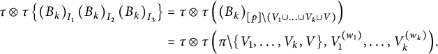 $$ \begin{align*} \tau\otimes \tau\left\{\left(B_k\right)_{I_1}\left(B_k\right)_{I_2}\left(B_k\right)_{I_3}\right\}&=\tau\otimes\tau \left(\left(B_k\right)_{[p]\setminus\left(V_1\cup \ldots \cup V_k \cup V\right)}\right)\\ &=\tau\otimes \tau\left(\pi\setminus\{V_1,\ldots,V_k,V\},V_1^{(w_1)},\ldots,V_k^{(w_k)}\right)\hspace{-1.5pt}. \end{align*} $$
Proof of Proposition 5.4
Let
 $\pi \notin P_2^{\operatorname {bicon}}(p)$
, and let
$\pi \notin P_2^{\operatorname {bicon}}(p)$
, and let
 $2l^*+1$
be the length of the smallest odd cycle in the intersection graph of
$2l^*+1$
be the length of the smallest odd cycle in the intersection graph of
 $\pi $
. We denote
$\pi $
. We denote
 $V_1,\ldots , V_{2l^*+1} \in \pi $
(any) ordered sequence of blocks in this smallest odd cycle, where
$V_1,\ldots , V_{2l^*+1} \in \pi $
(any) ordered sequence of blocks in this smallest odd cycle, where
 $V_{j}$
crosses
$V_{j}$
crosses
 $V_{j+1}$
for each
$V_{j+1}$
for each
 $j=1,\ldots ,2l^*+1$
and
$j=1,\ldots ,2l^*+1$
and
 $V_{2l^*+2}:=V_1$
. We first remove the first block
$V_{2l^*+2}:=V_1$
. We first remove the first block
 $V_1$
, and by Lemma 5.5 we get that
$V_1$
, and by Lemma 5.5 we get that
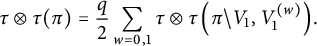 $$ \begin{align*} \tau\otimes\tau(\pi)=\frac{q}{2}\sum_{w=0,1}\tau\otimes\tau\left(\pi\setminus V_1,V_1^{(w)}\right)\hspace{-1.5pt}. \end{align*} $$
However, as it is the first block we remove, the distribution of
 $B_0=(b_{i_j})_{j \in [p]}$
is symmetric in both legs. In particular, we have
$B_0=(b_{i_j})_{j \in [p]}$
is symmetric in both legs. In particular, we have
 $$ \begin{align*} B_1(V_1^{(0)})\overset{d}{=}B_1(V_1^{(1)}), \end{align*} $$
and
 $$ \begin{align*} \tau\otimes\tau\left(\pi\setminus V_1,V_1^{(0)}\right)=\tau\otimes\tau\left(\pi\setminus V_1,V_1^{(1)}\right)\hspace{-1.5pt}. \end{align*} $$
Hence
 $$ \begin{align*} \tau\otimes\tau(\pi)=q\tau\otimes\tau\left(\pi\setminus V_1,V_1^{(0)}\right)\hspace{-1.5pt}. \end{align*} $$
We then fix the color of
 $V_1$
to be
$V_1$
to be
 $w_1=0$
. We aim to show by induction that the colors
$w_1=0$
. We aim to show by induction that the colors
 $w_1,w_2,\ldots ,w_{2l^*}$
of
$w_1,w_2,\ldots ,w_{2l^*}$
of
 $V_1,\ldots ,V_{2l^*}$
are deterministic and alternating,
$V_1,\ldots ,V_{2l^*}$
are deterministic and alternating,
 $$ \begin{align*} w=(w_1,\ldots,w_{2l^*})=(0,1,0,\ldots,1), \end{align*} $$
and so is
 $\theta ^{(k+1)}:=\theta \left (V_k,V_1^{(w_1)},\ldots ,V_{k}^{(w_{k})}\right )$
for
$\theta ^{(k+1)}:=\theta \left (V_k,V_1^{(w_1)},\ldots ,V_{k}^{(w_{k})}\right )$
for
 $1 \le k \le 2l^*$
in the sense that
$1 \le k \le 2l^*$
in the sense that
 $$ \begin{align*} \left(\theta^{(2)}_2,\theta^{(3)}_3,\theta^{(4)}_2,\ldots,\theta^{(2l^*)}_2\right)=(1,1,1,\ldots,1). \end{align*} $$
First, as
 $V_2$
crosses
$V_2$
crosses
 $V_1$
and
$V_1$
and
 $w_1=0$
, we have
$w_1=0$
, we have
 $\theta ^{(2)}_2=1$
. By Lemma 5.6, we have
$\theta ^{(2)}_2=1$
. By Lemma 5.6, we have
 $w_2=1$
. Suppose then that the result holds for some
$w_2=1$
. Suppose then that the result holds for some
 $1 < k < 2l^*$
. Let us prove that it also holds for
$1 < k < 2l^*$
. Let us prove that it also holds for
 $k+1$
. To simplify the reading, let us divide into two cases whether k is even or odd.
$k+1$
. To simplify the reading, let us divide into two cases whether k is even or odd.
Case k is even. The induction hypothesis implies that
 $$ \begin{align*} &(w_2,w_3,\ldots,w_k)=(1,0,\ldots,1);\\ &\left(\theta^{(2)}_2,\theta^{(3)}_3,\theta^{(4)}_2,\ldots,\theta^{(k)}_2\right)=(1,1,1,\ldots,1). \end{align*} $$
Since
 $V_{k+1}$
crosses
$V_{k+1}$
crosses
 $V_k$
, we automatically have that
$V_k$
, we automatically have that
 $\theta ^{(k+1)}_1=0$
. Moreover, as
$\theta ^{(k+1)}_1=0$
. Moreover, as
 $w_k=1$
, the definition of
$w_k=1$
, the definition of
 $\theta $
implies that
$\theta $
implies that
 $$ \begin{align*} \theta^{(k+1)}_2=0. \end{align*} $$
Hence either
 $\theta ^{(k+1)}_4=1$
or
$\theta ^{(k+1)}_4=1$
or
 $\theta ^{(k+1)}_3=1$
. Now consider all blocks
$\theta ^{(k+1)}_3=1$
. Now consider all blocks
 $V_{j_t}$
that might potentially cross
$V_{j_t}$
that might potentially cross
 $V_{k+1}$
, for
$V_{k+1}$
, for
 $j_t\le k$
. Since
$j_t\le k$
. Since
 $2l^*+1$
is the length of the smallest odd cycle, the cycles
$2l^*+1$
is the length of the smallest odd cycle, the cycles
 $(V_{j_t},\ldots , V_{k}, V_{k+1})$
are of even length. By a parity check,
$(V_{j_t},\ldots , V_{k}, V_{k+1})$
are of even length. By a parity check,
 $j_t$
must be even, and hence
$j_t$
must be even, and hence
 $$ \begin{align*} w_{j_t}=1. \end{align*} $$
This implies that all crossing blocks
 $V_{j_t}$
of
$V_{j_t}$
of
 $V_{k+1}$
for
$V_{k+1}$
for
 $j_t \le k$
have the same color
$j_t \le k$
have the same color
 $w_{j_t}=1$
. In particular, we have
$w_{j_t}=1$
. In particular, we have
 $$ \begin{align*} \theta^{(k+1)}_{3}=1. \end{align*} $$
We then apply Lemma 5.7 to get that
 $w_{k+1}=0$
.
$w_{k+1}=0$
.
Case k is odd. This follows similarly to the even case. We first have that
 $\theta ^{(k+1)}_1=0$
and as
$\theta ^{(k+1)}_1=0$
and as
 $w_{k}=0$
, we have
$w_{k}=0$
, we have
 $$ \begin{align*} \theta^{(k+1)}_3=0. \end{align*} $$
By the parity check on the even cycles
 $V_{k+1}$
might belong to, all crossing blocks
$V_{k+1}$
might belong to, all crossing blocks
 $V_{j_t}$
of
$V_{j_t}$
of
 $V_{k+1}$
for
$V_{k+1}$
for
 $j_t \le k$
have the same color
$j_t \le k$
have the same color
 $w_{j_t}=0$
. Hence
$w_{j_t}=0$
. Hence
 $$ \begin{align*} \theta^{(k+1)}_2=1, \end{align*} $$
and Lemma 5.6 implies that
 $w_{k+1}=1$
. This finishes the induction.
$w_{k+1}=1$
. This finishes the induction.
To conclude the proof, the block
 $V_{2l^*+1}$
crosses both
$V_{2l^*+1}$
crosses both
 $V_1$
of color
$V_1$
of color
 $w_1=0$
and
$w_1=0$
and
 $V_{2l^*}$
of color
$V_{2l^*}$
of color
 $w_{2l^*}=1$
. Hence
$w_{2l^*}=1$
. Hence
 $$ \begin{align*} \theta^{(2l^*+1)}_4=1. \end{align*} $$
Lemma 5.8 applied to
 $V=V_{2l^*+1}$
implies that
$V=V_{2l^*+1}$
implies that
 $$ \begin{align*} \tau\otimes\tau\left(\pi\setminus \{V_1,\ldots,V_{2l^*}\},V_1^{(0)},\ldots,V_{2l^*}^{(1)}\right)=0. \end{align*} $$
Applying Lemma 5.6 for blocks
 $V=V_k$
when k is even and Lemma 5.7 for
$V=V_k$
when k is even and Lemma 5.7 for
 $V=V_k$
when k is odd, we get that
$V=V_k$
when k is odd, we get that
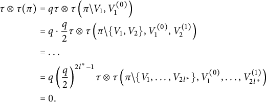 $$ \begin{align*} \tau\otimes \tau(\pi)&=q\tau\otimes \tau\left(\pi\setminus V_1,V_1^{(0)}\right)\\ &=q\cdot \frac{q}{2}\tau\otimes \tau\left(\pi\setminus\{V_1,V_2\},V_1^{(0)},V_2^{(1)}\right)\\ &=\ldots\\ &=q\left(\frac{q}{2}\right)^{2l^*-1}\tau\otimes \tau\left(\pi\setminus\{V_1,\ldots,V_{2l^*}\},V_1^{(0)},\ldots,V_{2l^*}^{(1)}\right)\\ &=0. \end{align*} $$
Therefore, for all
 $\pi \notin P_2^{\operatorname {bicon}}(p)$
, we have
$\pi \notin P_2^{\operatorname {bicon}}(p)$
, we have
 $\tau \otimes \tau (\pi )=0$
. This proves the first part of the proposition.
$\tau \otimes \tau (\pi )=0$
. This proves the first part of the proposition.
Assume now that
 $\pi \in P_2^{\operatorname {bicon}}(p)$
. Let
$\pi \in P_2^{\operatorname {bicon}}(p)$
. Let
 $V_1,\ldots ,V_{p/2}$
be an ordering of the blocks of
$V_1,\ldots ,V_{p/2}$
be an ordering of the blocks of
 $\pi $
such that
$\pi $
such that
 $V_k$
crosses at least one
$V_k$
crosses at least one
 $V_j$
for
$V_j$
for
 $j<k$
and all k. This can always be done as
$j<k$
and all k. This can always be done as
 $\pi $
is connected. Let
$\pi $
is connected. Let
 $\mathcal {V}_1,\mathcal {V}_2$
be the bipartite sets of vertices of the intersection graph of
$\mathcal {V}_1,\mathcal {V}_2$
be the bipartite sets of vertices of the intersection graph of
 $\pi $
,
$\pi $
,
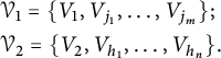 $$ \begin{align*} &\mathcal{V}_1=\{V_1,V_{j_1},\ldots,V_{j_m}\};\\ &\mathcal{V}_2=\{V_2,V_{h_1},\ldots,V_{h_n}\}. \end{align*} $$
Since
 $\pi $
is bipartite, if
$\pi $
is bipartite, if
 $V_k \in \mathcal {V}_1$
, all crossing blocks
$V_k \in \mathcal {V}_1$
, all crossing blocks
 $V_j$
of
$V_j$
of
 $V_k$
belong to
$V_k$
belong to
 $\mathcal {V}_2$
, and similarly if
$\mathcal {V}_2$
, and similarly if
 $V_k \in \mathcal {V}_2$
. We assume again that the color of
$V_k \in \mathcal {V}_2$
. We assume again that the color of
 $V_1$
is
$V_1$
is
 $w_1=0$
, since
$w_1=0$
, since
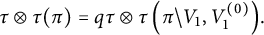 $$ \begin{align*} \tau\otimes \tau(\pi)=q \tau\otimes\tau \left(\pi\setminus V_1,V_1^{(0)}\right)\hspace{-1.5pt}. \end{align*} $$
We will prove that both the color
 $w_k$
and the binary vector
$w_k$
and the binary vector
 $\theta ^{(k)}$
of
$\theta ^{(k)}$
of
 $V_k$
depend only on which bipartite set
$V_k$
depend only on which bipartite set
 $V_k$
belongs to, namely, for all
$V_k$
belongs to, namely, for all
 $k \ge 2$
, the following hold.
$k \ge 2$
, the following hold.
-
(1) If
$V_k \in \mathcal {V}_1$
, then
$w_k=0$
and
$\theta ^{(k)}_{3}=1$
; -
(2) Otherwise,
$V_k \in \mathcal {V}_2$
,
$w_k=1$
and
$\theta ^{(k)}_2=1$
.


Indeed, note first that
 $V_2 \in \mathcal {V}_2$
,
$V_2 \in \mathcal {V}_2$
,
 $\theta ^{(2)}_2=1$
as it crosses
$\theta ^{(2)}_2=1$
as it crosses
 $V_1$
and
$V_1$
and
 $w_1=0$
. Then, Lemma 5.6 implies that
$w_1=0$
. Then, Lemma 5.6 implies that
 $w_2=1$
. Assume then that the result holds for some l and for all
$w_2=1$
. Assume then that the result holds for some l and for all
 $1 \le k \le l$
. Let us prove that it holds for
$1 \le k \le l$
. Let us prove that it holds for
 $V_{l+1}$
as well. Indeed, assume without loss of generality that
$V_{l+1}$
as well. Indeed, assume without loss of generality that
 $V_{l+1} \in \mathcal {V}_1$
. Then
$V_{l+1} \in \mathcal {V}_1$
. Then
 $V_{l+1}$
only crosses blocks
$V_{l+1}$
only crosses blocks
 $V_{j_t}$
such that
$V_{j_t}$
such that
 $V_{j_t} \in \mathcal {V}_2$
, for
$V_{j_t} \in \mathcal {V}_2$
, for
 $j_t \le l$
. Since all colors
$j_t \le l$
. Since all colors
 $w_{j_t}=1$
, we deduce that
$w_{j_t}=1$
, we deduce that
 $$ \begin{align*} \theta^{(l+1)}_3=1. \end{align*} $$
Then, Lemma 5.7 implies that
 $w_{l+1}=0$
and induction is proved. We then apply Lemma 5.5 for
$w_{l+1}=0$
and induction is proved. We then apply Lemma 5.5 for
 $V_1$
, Lemma 5.6 for all blocks
$V_1$
, Lemma 5.6 for all blocks
 $V_k \in \mathcal {V}_2$
and Lemma 5.7 for all blocks
$V_k \in \mathcal {V}_2$
and Lemma 5.7 for all blocks
 $V_k \in \mathcal {V}_1$
for
$V_k \in \mathcal {V}_1$
for
 $k \ge 2$
, so that
$k \ge 2$
, so that
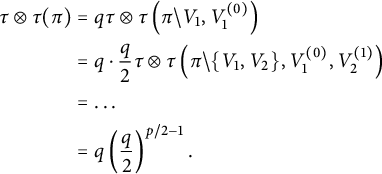 $$ \begin{align*} \tau\otimes \tau(\pi)&=q\tau\otimes \tau\left(\pi\setminus V_1,V_1^{(0)}\right)\\ &=q\cdot \frac{q}{2}\tau\otimes \tau\left(\pi\setminus\{V_1,V_2\},V_1^{(0)},V_2^{(1)}\right)\\ &=\ldots\\ &=q\left(\frac{q}{2}\right)^{p/2-1}. \end{align*} $$
It follows then that
 $$ \begin{align*} \tau\otimes \tau(\pi)=q\left(\frac{q}{2}\right)^{p/2-1}=2\left(\frac{q}{2}\right)^{p/2}, \end{align*} $$
and the result is proved.
5.4 Proof of Theorem 1.1
We are now ready to prove the main theorem. Recall that
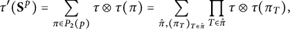 $$ \begin{align*} \tau'(\mathbf{{S}}^{p})=\sum_{\pi \in P_2(p)}\tau\otimes \tau(\pi)= \sum_{\hat{\pi},(\pi_T)_{T \in \hat{\pi}}}\prod_{T \in \hat{\pi}}\tau\otimes \tau(\pi_T), \end{align*} $$
where the second summation runs over
 $(\hat {\pi },(\pi _T)_{T \in \hat {\pi }})\in \Phi (P_2(p))$
, using the bijection
$(\hat {\pi },(\pi _T)_{T \in \hat {\pi }})\in \Phi (P_2(p))$
, using the bijection
 $\Phi $
defined in (4). Note that if
$\Phi $
defined in (4). Note that if
 $|T|=2$
, then by Corollary 5.2 we have
$|T|=2$
, then by Corollary 5.2 we have
 $\tau \otimes \tau (\pi _T)=1$
. Therefore, we deduce that
$\tau \otimes \tau (\pi _T)=1$
. Therefore, we deduce that
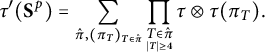 $$ \begin{align*} \tau'(\mathbf{{S}}^{p})= \sum_{\hat{\pi},(\pi_T)_{T \in \hat{\pi}}} \prod_{\underset{|T|\geq 4}{T \in \hat{\pi}}}\tau\otimes \tau(\pi_T). \end{align*} $$
Using Proposition 5.4, we get
 $$ \begin{align*} \tau'(\mathbf{{S}}^{p})= \sum_{\hat{\pi}\in NC(p)}\sum_{(\pi_T)_{T \in \hat{\pi}}}\prod_{\underset{|T|\geq 4}{T \in \hat{\pi}}}2 \Big(\frac{q}{2}\Big)^{\frac{|T|}{2}}, \end{align*} $$
where the second summation runs over bipartite connected pair partitions
 $\pi _T$
, for
$\pi _T$
, for
 $T \in \hat {\pi }$
. Finally, note that the number of size-two blocks is precisely
$T \in \hat {\pi }$
. Finally, note that the number of size-two blocks is precisely
 $\mathbf {ncr}(\pi )$
and thus
$\mathbf {ncr}(\pi )$
and thus
 $$ \begin{align*} &|\{T \in \hat{\pi}:|T| \ge 4\}|=\mathbf{cc}(\pi)-\mathbf{ncr}(\pi). \end{align*} $$
Since
 $$ \begin{align*}\sum_{\substack{T \in \hat{\pi}\\ |T| \ge 4}}\frac{|T|}{2}=\mathbf{cr}(\pi), \end{align*} $$
using again the bijection
 $\Phi $
, we deduce that
$\Phi $
, we deduce that
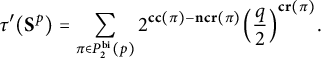 $$ \begin{align*} \tau'(\mathbf{{S}}^{p})= \sum_{\pi \in P_2^{\operatorname{bi}}(p)} 2^{\mathbf{cc}(\pi)-\mathbf{ncr}(\pi)} \Big(\frac{q}{2}\Big)^{\mathbf{cr}(\pi)}. \end{align*} $$
This finishes the proof in view of Proposition 3.3 and of the fact that
 $$ \begin{align*} \mathbf{ncr}(\pi)+\mathbf{cr}(\pi)=|\pi|=\frac{p}{2}. \end{align*} $$
6 Alternative proof
In this section, we provide a short alternative proof of Theorem 1.1. Let us denote
 $a_k^\circ =a_k-\lambda $
the centering of
$a_k^\circ =a_k-\lambda $
the centering of
 $a_k$
. Hence
$a_k$
. Hence
 $$ \begin{align*} a_k\otimes a_k=(a_k^\circ+\lambda)\otimes (a_k^\circ+\lambda). \end{align*} $$
In particular, we have
 $$ \begin{align} a_k\otimes a_k-\lambda^2=a_k^\circ\otimes a_k^\circ+\lambda a_k^\circ \otimes 1+\lambda 1\otimes a_k^\circ. \end{align} $$
Let
 $$ \begin{align} &S_n^{(1)}=\frac{1}{\sqrt{n}}\sum_{k\in [n]}a_k^{(1)}:=\frac{1}{\sqrt{n}}\sum_{k\in [n]}a_k^\circ \otimes a_k^\circ; \end{align} $$
 $$ \begin{align} &S_n^{(2)}=\frac{1}{\sqrt{n}}\sum_{k\in [n]}a_k^{(2)}:=1\otimes\left(\frac{1}{\sqrt{n}}\sum_{k\in [n]} a_k^\circ\right); \end{align} $$
 $$ \begin{align} &S_n^{(3)}=\frac{1}{\sqrt{n}}\sum_{k\in [n]}a_k^{(3)}:=\left(\frac{1}{\sqrt{n}}\sum_{k\in [n]} a_k^\circ\right)\otimes 1. \end{align} $$
Then, we deduce by (16) that
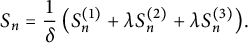 $$ \begin{align*} S_n=\frac{1}{\delta}\left(S_n^{(1)}+\lambda S_n^{(2)}+\lambda S_n^{(3)}\right)\hspace{-1.5pt}. \end{align*} $$
The following lemma computes the limiting law of
 $S_n^{(i)}$
.
$S_n^{(i)}$
.
Lemma 6.1 Let
 $a,a_1,\ldots ,a_n$
be free identically distributed random variables with mean
$a,a_1,\ldots ,a_n$
be free identically distributed random variables with mean
 $\lambda =\tau (a)$
and variance
$\lambda =\tau (a)$
and variance
 $\sigma ^2=\operatorname {var}(a)$
. Let
$\sigma ^2=\operatorname {var}(a)$
. Let
 $S_n^{(i)}$
as in (17) for
$S_n^{(i)}$
as in (17) for
 $i=1,2,3$
. Then, the following hold.
$i=1,2,3$
. Then, the following hold.
-
(1)
$S_n^{(1)}$
converges to a semi-circle random variable with variance
$\sigma ^4$
. -
(2)
$S_n^{(2)}$
converges to a semi-circle random variable with variance
$\sigma ^2$
. -
(3)
$S_n^{(3)}$
converges to a semi-circle random variable with variance
$\sigma ^2$
.


Proof Let
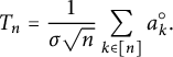 $$ \begin{align*} T_n=\frac{1}{\sigma\sqrt{n}}\sum_{k\in [n]}a_k^\circ. \end{align*} $$
We first note that for any
 $p \ge 1$
, we have
$p \ge 1$
, we have
 $$ \begin{align*} \tau \otimes \tau \left((S_n^{(2)})^p\right)=\tau \otimes \tau \left((S_n^{(3)})^p\right)=\sigma^p\tau(T_n^p). \end{align*} $$
Hence, Voiculescu’s Free Central Limit Theorem implies that
 $S_n^{(i)}/\sigma $
converges to a standard semi-circle random variable
$S_n^{(i)}/\sigma $
converges to a standard semi-circle random variable
 $s_i$
, for
$s_i$
, for
 $i=2,3$
. Secondly, note that
$i=2,3$
. Secondly, note that
 $(a_k^{(1)})_k$
are exchangeable and centered. It also follows immediately by the tensor structure that the centering condition
$(a_k^{(1)})_k$
are exchangeable and centered. It also follows immediately by the tensor structure that the centering condition
 $$ \begin{align*} \tau\otimes\tau(a_{i_1}^{(1)}\ldots a_{i_p}^{(1)})=0 \end{align*} $$
holds whenever there exists an index
 $i_k$
different from the others. We can then apply [Reference Bożejko and Speicher3, Theorem 0] to get that
$i_k$
different from the others. We can then apply [Reference Bożejko and Speicher3, Theorem 0] to get that
 $S_n^{(1)}$
converges and
$S_n^{(1)}$
converges and
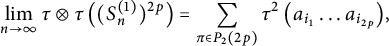 $$ \begin{align*} \lim_{n \to \infty}\tau \otimes \tau \left((S_n^{(1)})^{2p}\right)=\sum_{\pi \in P_2(2p)}\tau^2 \left(a_{i_1}\ldots a_{i_{2p}}\right)\hspace{-1.5pt}, \end{align*} $$
where
 $\ker i=\pi $
. Now, by Voiculescu’s Free Central Limit Theorem, we get that
$\ker i=\pi $
. Now, by Voiculescu’s Free Central Limit Theorem, we get that
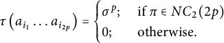 $$ \begin{align*} \tau\left(a_{i_1}\ldots a_{i_{2p}}\right)= \begin{cases} \sigma^p;& \text{ if } \pi \in NC_2(2p)\\ 0;& \text{ otherwise.} \end{cases} \end{align*} $$
We then get that
 $S_n^{(1)}/\sigma ^2$
converges to a standard semi-circle law
$S_n^{(1)}/\sigma ^2$
converges to a standard semi-circle law
 $s_1$
.
$s_1$
.
Now, we prove that the tuple
 $(S_n^{(1)},S_n^{(2)},S_n^{(3)})$
converges in distribution.
$(S_n^{(1)},S_n^{(2)},S_n^{(3)})$
converges in distribution.
Lemma 6.2 Let
 $a,a_1,\ldots ,a_n$
be free identically distributed random variables with mean
$a,a_1,\ldots ,a_n$
be free identically distributed random variables with mean
 $\lambda =\tau (a)$
and variance
$\lambda =\tau (a)$
and variance
 $\sigma ^2=\operatorname {var}(a)$
. Let
$\sigma ^2=\operatorname {var}(a)$
. Let
 $S_n^{(i)}$
as in (17) for
$S_n^{(i)}$
as in (17) for
 $i=1,2,3$
. Then the tuple
$i=1,2,3$
. Then the tuple
 $(S_n^{(1)},S_n^{(2)},S_n^{(3)})$
converges in distribution.
$(S_n^{(1)},S_n^{(2)},S_n^{(3)})$
converges in distribution.
Proof We must prove that for any
 $i \in \{1,2,3\}^p$
, the limit of
$i \in \{1,2,3\}^p$
, the limit of
 $\tau \otimes \tau \left (S_n^{(i_1)}\ldots S_n^{(i_p)}\right )$
exists when n goes to infinity. We write
$\tau \otimes \tau \left (S_n^{(i_1)}\ldots S_n^{(i_p)}\right )$
exists when n goes to infinity. We write
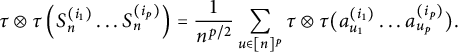 $$ \begin{align*} \tau\otimes \tau \left(S_n^{(i_1)}\ldots S_n^{(i_p)}\right)=\frac{1}{n^{p/2}}\sum_{u\in [n]^{p}}\tau\otimes\tau(a_{u_1}^{(i_1)}\ldots a_{u_p}^{(i_p)}). \end{align*} $$
We can as usual decompose the summation according to
 $\ker u \in P(p)$
, hence
$\ker u \in P(p)$
, hence
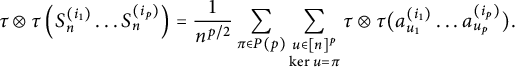 $$ \begin{align*} \tau\otimes \tau \left(S_n^{(i_1)}\ldots S_n^{(i_p)}\right)=\frac{1}{n^{p/2}}\sum_{\pi \in P(p)}\sum_{\substack{u \in [n]^p\\ \ker u=\pi}}\tau\otimes\tau(a_{u_1}^{(i_1)}\ldots a_{u_p}^{(i_p)}). \end{align*} $$
We note that
 $\tau \otimes \tau (a_{u_1}^{(i_1)}\ldots a_{u_p}^{(i_p)})$
only depends on
$\tau \otimes \tau (a_{u_1}^{(i_1)}\ldots a_{u_p}^{(i_p)})$
only depends on
 $\pi $
and i. Let us denote this value by
$\pi $
and i. Let us denote this value by
 $\tau \otimes \tau (\pi , i)$
. We then have
$\tau \otimes \tau (\pi , i)$
. We then have
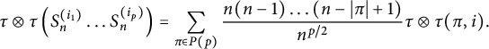 $$ \begin{align*} \tau\otimes \tau \left(S_n^{(i_1)}\ldots S_n^{(i_p)}\right)=\sum_{\pi \in P(p)}\frac{n(n-1)\ldots (n-|\pi|+1)}{n^{p/2}}\tau\otimes\tau(\pi,i). \end{align*} $$
It is immediate to check that if
 $V=\{v\}\in \pi $
has a block of size one, we have
$V=\{v\}\in \pi $
has a block of size one, we have
 $$ \begin{align*} \tau\otimes\tau(\pi,i)=0 \end{align*} $$
Moreover, if there exists
 $V\in \pi $
with
$V\in \pi $
with
 $|V| \ge 3$
, its contribution is going to zero. We deduce that
$|V| \ge 3$
, its contribution is going to zero. We deduce that
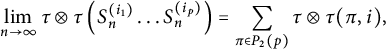 $$ \begin{align} \lim_{n\to \infty}\tau\otimes \tau \left(S_n^{(i_1)}\ldots S_n^{(i_p)}\right)=\sum_{\pi \in P_2(p)}\tau\otimes\tau(\pi,i), \end{align} $$
and the proof is finished.
Therefore, Lemmas 6.1 and 6.2 imply that the tuple
 $(S_n^{(1)},S_n^{(2)},S_n^{(3)})$
converges in distribution to
$(S_n^{(1)},S_n^{(2)},S_n^{(3)})$
converges in distribution to
 $(\sigma ^2s_1,\sigma s_2,\sigma s_3)$
. The following final lemma allows us to understand the joint law of
$(\sigma ^2s_1,\sigma s_2,\sigma s_3)$
. The following final lemma allows us to understand the joint law of
 $(s_1,s_2,s_3)$
.
$(s_1,s_2,s_3)$
.
Lemma 6.3 Let
 $a,a_1,\ldots ,a_n$
be free identically distributed random variables with mean
$a,a_1,\ldots ,a_n$
be free identically distributed random variables with mean
 $\lambda =\tau (a)$
and variance
$\lambda =\tau (a)$
and variance
 $\sigma ^2=\operatorname {var}(a)$
. Let
$\sigma ^2=\operatorname {var}(a)$
. Let
 $S_n^{(i)}$
as in (17) for
$S_n^{(i)}$
as in (17) for
 $i=1,2,3$
. Let
$i=1,2,3$
. Let
 $(\sigma ^2s_1,\sigma s_2,\sigma s_3)$
be their joint limiting law. Then, the following holds.
$(\sigma ^2s_1,\sigma s_2,\sigma s_3)$
be their joint limiting law. Then, the following holds.
-
(1) The variables
$s_2,s_3$
are classical independent. -
(2)
$s_1$
is free from both
$s_2$
and
$s_3$
.


Proof By definition, we note that
 $$ \begin{align*} S_n^{(2)}S_n^{(3)}=S_n^{(3)}S_n^{(2)}. \end{align*} $$
Hence,
 $S_n^{(2)}$
and
$S_n^{(2)}$
and
 $S_n^{(3)}$
are classical independent and commute as the trace factorizes, i.e.,
$S_n^{(3)}$
are classical independent and commute as the trace factorizes, i.e.,
 $$ \begin{align*} \tau\otimes \tau \left((S_n^{(2)})^p(S_n^{(3)})^q\right)=\tau\left((S_n^{(2)})^p\right)\tau\left((S_n^{(3)})^q\right)\hspace{-1.5pt}. \end{align*} $$
This implies that
 $s_2$
and
$s_2$
and
 $s_3$
are classical independent. Let us prove now that
$s_3$
are classical independent. Let us prove now that
 $s_1$
is free from
$s_1$
is free from
 $s_2$
. By definition, we need to show that for any
$s_2$
. By definition, we need to show that for any
 $i_1\ne i_2 \ne \ldots \ne i_p$
in
$i_1\ne i_2 \ne \ldots \ne i_p$
in
 $\{1,2\}$
, we get
$\{1,2\}$
, we get
 $$ \begin{align*} \lim_{n \to \infty}\tau\otimes \tau \left(S_n^{(i_1)}\ldots S_n^{(i_p)}\right)=\tau \left(s_{i_1}\ldots s_{i_p}\right)=0. \end{align*} $$
By (18), we get
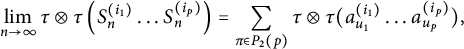 $$ \begin{align*} \lim_{n\to \infty}\tau\otimes \tau \left(S_n^{(i_1)}\ldots S_n^{(i_p)}\right)=\sum_{\pi \in P_2(p)}\tau\otimes\tau(a_{u_1}^{(i_1)}\ldots a_{u_{p}}^{(i_p)}), \end{align*} $$
where
 $\ker u=\pi $
. Therefore, it suffices to prove that for any pair partition
$\ker u=\pi $
. Therefore, it suffices to prove that for any pair partition
 $\pi \in P_2(p)$
, any alternating sequence
$\pi \in P_2(p)$
, any alternating sequence
 $i_1 \ne i_2 \ne \ldots \ne i_p$
in
$i_1 \ne i_2 \ne \ldots \ne i_p$
in
 $\{1,2\}$
and any
$\{1,2\}$
and any
 $u\in [n]^p$
such that
$u\in [n]^p$
such that
 $\ker u=\pi $
, we have
$\ker u=\pi $
, we have
 $$ \begin{align*} \tau\otimes\tau(a_{u_1}^{(i_1)}\ldots a_{u_p}^{(i_p)})=0. \end{align*} $$
To this end, we can assume by cyclicity that
 $i_1=i_3=\ldots =i_{p-1}=1$
and
$i_1=i_3=\ldots =i_{p-1}=1$
and
 $i_2=i_4=\ldots =i_p=2$
. Then
$i_2=i_4=\ldots =i_p=2$
. Then
 $$ \begin{align*} \tau\otimes\tau(a_{u_1}^{(i_1)}\ldots a_{u_p}^{(i_p)})=\tau(a_{u_1}a_{u_2}\ldots a_{u_p})\tau(a_{u_1}a_{u_3}\ldots a_{u_{p-1}}). \end{align*} $$
As
 $\pi \in P_2(p)$
and
$\pi \in P_2(p)$
and
 $\ker u=\pi $
, we have
$\ker u=\pi $
, we have
 $$ \begin{align*} \tau\left(a_{u_1}\ldots a_{u_{p}}\right)= \begin{cases} \sigma^{p/2};& \text{ if } \pi \in NC_2(p)\\ 0;& \text{ otherwise.} \end{cases} \end{align*} $$
However, suppose
 $\pi \in NC_2(p)$
. Then, there exists an interval block
$\pi \in NC_2(p)$
. Then, there exists an interval block
 $\{j,j+1\}\in \pi $
. Let us suppose without loss of generality that j is odd (otherwise, take
$\{j,j+1\}\in \pi $
. Let us suppose without loss of generality that j is odd (otherwise, take
 $j+1$
instead). We then have
$j+1$
instead). We then have
 $u_j=u_{j+1} \ne u_{l}$
for all
$u_j=u_{j+1} \ne u_{l}$
for all
 $l \notin \{j,j+1\}$
. But then
$l \notin \{j,j+1\}$
. But then
 $a_{u_j}$
is free independent from
$a_{u_j}$
is free independent from
 $$ \begin{align*} a_{u_1},a_{u_3},\ldots,a_{u_{j-2}},a_{u_{j+2}},\ldots,a_{u_{p-1}}. \end{align*} $$
Hence
 $$ \begin{align*} \tau(a_{u_1}a_{u_3}\ldots a_{u_{p-1}})=\tau(a_{u_j})\tau(a_{u_1}\ldots a_{u_{j-2}}a_{u_{j+2}}\ldots a_{u_{p-1}})=0. \end{align*} $$
Therefore, for all
 $\pi \in P_2(p)$
and
$\pi \in P_2(p)$
and
 $u\in [n]^p$
such that
$u\in [n]^p$
such that
 $\ker u=\pi $
, we have
$\ker u=\pi $
, we have
 $$ \begin{align*} \tau\otimes\tau(a_{u_1}^{(i_1)}\ldots a_{u_p}^{(i_p)})=0, \end{align*} $$
and it follows that
 $s_1$
is free from
$s_1$
is free from
 $s_2$
. By symmetry, it is also free from
$s_2$
. By symmetry, it is also free from
 $s_3$
and the result follows.
$s_3$
and the result follows.
We can now conclude the alternative proof of Theorem 1.1.
Proof of Theorem 1.1
 $$ \begin{align*} S_n=\frac{1}{\delta}\left(S_n^{(1)}+\lambda S_n^{(2)}+\lambda S_n^{(3)}\right)\hspace{-1.5pt}. \end{align*} $$
Moreover, Lemmas 6.1 and 6.2 imply that
 $(S_n^{(1)},S_n^{(2)},S_n^{(3)})$
converges in distribution to
$(S_n^{(1)},S_n^{(2)},S_n^{(3)})$
converges in distribution to
 $(\sigma ^2 s_1,\sigma s_2,\sigma s_3)$
, where each
$(\sigma ^2 s_1,\sigma s_2,\sigma s_3)$
, where each
 $s_i$
is a standard semi-circle random variable. Finally, Lemma 6.3 implies that
$s_i$
is a standard semi-circle random variable. Finally, Lemma 6.3 implies that
 $s_1$
is free from
$s_1$
is free from
 $(s_2,s_3)$
, and
$(s_2,s_3)$
, and
 $s_2$
is classical independent from
$s_2$
is classical independent from
 $s_3$
. Then,
$s_3$
. Then,
 $S_n$
converges in distribution
$S_n$
converges in distribution
 $$ \begin{align*} S_n \Rightarrow \frac{1}{\delta}\left(\sigma^2 s_1 +\lambda\sigma s_2+\lambda\sigma s_3\right)\hspace{-1.5pt}. \end{align*} $$
The definition of q and symmetry of
 $s_2,s_3$
imply that
$s_2,s_3$
imply that
 $$ \begin{align*} \frac{1}{\delta}\left(\sigma^2 s_1 +\lambda\sigma s_2+\lambda\sigma s_3\right)=\sqrt{1-q}s_1+\sqrt{\frac{q}{2}}s_2+\sqrt{\frac{q}{2}}s_3. \end{align*} $$
This finishes the proof.
Acknowledgments
The last named author would like to thank Guillaume Cébron and Roland Speicher for helpful discussions. The second named author also thanks Philippe Biane for useful discussions. We thank the anonymous reviewer for generously communicating the alternative proof.


