


Introduction
All planetary rovers are mobile scientific instrument platforms – scientific investigation is their raison d'etre. Robotics has much to contribute to the pursuit of planetary science, including astrobiology in the context of planetary exploration. However, robotic astrobiology is still nascent and underdeveloped despite its promise. This review of the current state-of-the-art and discussion of the prospects and future directions of robotic astrobiology is focused on Mars rover missions. It is neither comprehensive nor objective, but it is hoped that it will stimulate further developments. The primary objective of robotic astrobiology is to marshal techniques of robotics to serve the astrobiology quest by enhancing the scientific productivity of Mars rover missions. The long-term objective is to create a ‘robotic astrobiologist’ facility on board future planetary rovers that can match or exceed the capabilities of human astrobiologists on Earth. This will enormously increase the scientific productivity of rover missions by allowing the rover to make decisions on selecting high priority targets and the appropriate methods of interrogation of the target using a judiciously selected set of scientific instruments onboard. This constitutes the back-engine of this facility to implement decision-making based on scientific classifications equivalent to the combined expertise of human scientists. Of course, the human scientist at the Earth station will remain the overseer. The short-term objective is to focus on the front end of such a facility – signal processing of camera images in order to classify rocks. Our principal tool for these investigations is the 30 kg Kapvik microrover designed from an earlier concept for a Mars microrover as part of a low-cost Mars mission (Ellery et al. Reference Ellery, Ball, Cockell, Dickensheets, Edwards, Kolb, Lammer, Patel and Richter2004a, Reference Ellery, Wynn-Williams, Parnell, Edwards and Dickensheetsb, Reference Ellery, Richter, Parnell and Baker2006) (Fig. 1).
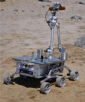
Fig. 1. Kapvik micro-rover at the Canadian Space Agency's Mars Yard.
Kapvik (Inuit word for wolverine, a rather ferocious small mammal native to the Canadian north) was developed for the CSA (Canadian Space Agency) by an industry–academia consortium, the mechanical design of which is described in Setterfield et al. (Reference Setterfield, Ellery and Frazier2014), while aspects of its electronics architecture is described in Cross et al. (Reference Cross, Nicol, Qadi and Ellery2013). There are several novel features in its design. It implements an instrumented rocker-bogie chassis permitting online traction analysis during traverse (Setterfield & Ellery Reference Setterfield and Ellery2013). Furthermore, it adopts an integrated manipulator-scoop/camera mast system (Liu et al. Reference Liu, Liu, Zhang, Gao, Yuan and Zheng2015a, Reference Liu, Lui, Zhang, Gao, Yuan and Zhengb). FPGAs are the primary computing platform to implement stereovision and LIDAR processing with cubature Kalman filter and FastSLAM algorithms for autonomous navigation (Hewitt et al. Reference Hewitt, Ellery and de Ruiter2017). It is a fully functional end-to-end demonstrator rover platform with a clear path to flight qualification and is still operating successfully. It was deployed to investigate multiple scientific instrument-based operations in Mars-like geological sites pertinent to serpentine rock (Qadi et al. Reference Qadi, Cloutis, Samson, Whyte, Ellery, Bell, Berard, Boivin, Haddad and Lavoie2015), which has potential astrobiological significance (Parnell et al. Reference Parnell, Boyce and Blamey2010). It has been deployed with a magnetometer to investigate rover-deployed magnetic measurements (Hay et al. Reference Hay, Samson and Ellery2017).
Martian geology is diverse and complex. For instance, jarosite detected by Spirit in the Gusev crater indicates past aqueous acidic weathering conditions (preventing the deposition of carbonate minerals) (Hurowitz et al. Reference Hurowitz, McLennan, Tosca, Arvidson, Michalski, Ming, Schroder and Squyres2006). Martian soils have high concentrations of S and Cl suggesting sulphate and chloride evaporite salts over widely space geographical locations. Such sites are attractive as astrobiological targets – a viable sample of a Bacillus bacterial strain was reportedly recovered and cultured from a brine inclusion within a 250 million year old halite crystal of Salado New Mexico (Vreeland et al. Reference Vreeland, Rosenzweig and Powers2000). However, 16 s rDNA sequencing revealed that the bacteria closely resemble modern Salibacillus marismortui and was thus a contaminant (Maugham et al. Reference Maugham, Birky, Nicholson, Rosenszeig and Vreeland2002; Nickle et al. Reference Nickle, Learn, Rain, Mullins and Mittler2002; Willersley & Hebsgaard Reference Willersley and Hebsgaard2005). Nevertheless, evaporite deposits remain attractive as a source of palaeobiotic signatures. The Gale crater indicates neutral pH conditions – the Curiosity rover has detected fluvial–lacustrine mudstones as evidence of ancient lakes in the Gale crater that could have supported chemolithoautrophic life especially iron and sulphur species (Grotzinger & The MSL Science Team Reference Grotzinger2014). This Mars geological complexity has persisted over geological timescales. It has been determined from evidence of shoreline patterns that an ocean may have covered the northern plains of Mars (constituting one-third of the Martian surface) at least 2 Gy ago (Perron et al. Reference Perron, Mitrovica, Manga, Matsuyama and Richards2007). These are all potential astrobiological targets of great variety. Hydrothermal regions on Mars with characteristic carbonate, sulphate, sulphide and metal hydroxide/oxide deposits elicit high astrobiological potential (Schultze-Makuch et al. Reference Schultze-Makuch, Dohm, Fan, Fairen, Rodriiguez, Baker and Fink2007) – Tharsis region, impact craters such as Gusev (visited by Spirit) and Gale (visited by Curiosity), and gullies such as at the Hale crater. At close quarters, the identification of phyllosilicates, jarosite and haematite can be detected as evidence of aqueous activity from rovers. The ‘follow the water’ strategy adopted by NASA favours a search for such potentially habitable environments. Implicit in this strategy is the complex geological history and geography of Mars, which makes such a strategy a challenge to Martian rover missions. Our goal is to employ an exploration strategy that maximizes the scientific return of these missions that attempts – eventually – to incorporate sophisticated geological and astrobiological knowledge.
We take Mars sample return as our baseline mission concept for the deployment of a robotic astrobiology capability (MEPAD 2008). However, any Mars rover mission such as ExoMars can exploit the methods presented here. Certain types of high-resolution scientific measurement are more readily performed in laboratories rather than in situ – radiometric dating, isotopic analysis and life detection experiments, all of which require high stability and multiple samples. This favours the return of samples from Mars for laboratory analysis to supplement in situ measurements undertaken by Mars lander and rover missions to date. The question of the size of returned sample is debated ranging from 50 to 200 g as the minimum useful quantity, but larger samples of 1 kg are considered to be optimal. We can thus assume a baseline of 5–20 × 50–200 g samples for return. This allows a trade of sample diversity against sample size. In either case, site selection for the recovery of these samples will be paramount. Furthermore, the quality of the samples is more important than quantity. Samples returned from known explored locations provide geological context unlike meteorite samples – grab-and-go missions diminish the scientific value of returned samples. This favours the employment of in situ measurements and analysis to select samples to be returned and their context over a 6–12-month surface sortie. Non-destructive testing can be performed on samples prior to their return to Earth – camera imaging, microscopic imaging and mineralogical analysis (infrared and Raman spectroscopy). Destructive analysis may be formed on contextual samples – high-resolution imaging (scanning electron microscopy), mineralogy (X-ray reflectance and/or diffraction spectrometry), chemical/elemental analysis (gas chromatography and/or laser plasma spectroscopy), isotopic analysis (mass spectrometry), DNA extraction (electrophoresis), DNA sequencing (polymerase chain reaction), etc. Each returned sample will involve an enormous investment of exploration effort. It is essential that the samples are selected judiciously and that time and energy are not wasted wantonly by the current strategy of sample everything and deploy the entire suite of scientific instruments on all recovered samples. Judicious sampling requires prioritization of potential astrobiological targets (e.g. aqueous deposited sedimentary rock as potential repositories of fossils) over pure geological targets (e.g. igneous rock), favouring the deployment of non-destructive astrobiological analysis, e.g. infrared Raman spectroscopy could potentially detect biomolecules in fossils. Instruments with discrete count rates and low signal-to-noise ratio, which suffer from peak spreading by smoothing algorithms may benefit from Kalman filtering, e.g. Mossbauer spectroscopy (Albrecht et al. Reference Albrecht, Schwantes, Kukkadapu, McDonald, Eiden and Sweet2015). A Gaussian smoothing function of the form  $g(x) = (1/\sqrt {{\rm \sigma \pi}} ){\rm e}^{ - {(x - m)}^2/{\rm \sigma}} $ was passed through the Kalman filter as a process model. Raman spectroscopy would be a suitable instrument for such signal processing to enhance its response. Furthermore, the covariance matrix of the Kalman filter with its O(n 3) computational complexity may be compressed using an orthonormal wavelet transform with only O(n) coefficients reducing both the processing and storage requirements for the Kalman filter (Chin & Mariano Reference Chin and Mariano1994). The Kalman filter is a predictor–corrector algorithm that estimates noise from measurements and models (in the form of covariance matrices) to optimize estimates of the system dynamics and how it evolves over time. It is widely used in both aerospace and robotic control systems. Dynamic equations of a system denote a process model and measurements given by:
 $$x_i = Ax_{i - 1} + B_i + w_i,$$
 $$y_i = Cx_i + v_i,$$
where A = dynamic matrix, C = measurement matrix, w i and v i are zero-mean Gaussian random noise vectors with covariances of Q i and R i, respectively. The Kalman filter iteratively computes a statistically optimal estimate of x i. It computes in two stages:
Prediction stage:
 $$\bar x_i = A\hat x_{i - 1} + B_i,$$
 $$\bar P_i = A(A\hat P_{i - 1})^T + Q_i.$$
Update stage:
 $$K_i = \bar P_iC_i^T (C_i\bar P_iC_i^T + R_i)^{ - 1},$$
 $$\hat x_i = \bar x_i + K_i(y_i - C_i\bar x_i),$$
 $$\hat P_i = \bar P_i - K_iC_i\bar P_i,$$
where P i = covariance matrix of error between the predicted and measured process states K i = Kalman filter gain.
The prediction is based on the process model and previous filter estimates; the prediction is corrected by the error between the predicted and the measured states modified by the Kalman gain. The Kalman gain is calculated from the predicted state covariance and the noise covariances – it minimizes the difference between predicted and measured states of the system. The covariance matrix P and Kalman gain K should converge in a few steps under certain assumptions. The power of the Kalman filter lies in its ability to estimate a state in the presence of noise in both process and measurements. The selected samples to be returned should be preferably maintained below −20°C though maintenance below +20°C, which is considered acceptable. Heat sterilization of returned samples would seriously damage the scientific value of the samples, negating the endowment invested in their recovery (Fairen & Schulze-Makuch Reference Fairen and Schulze-Makuch2013).
Science phases of rover missions
Current Mars rover operations are hampered by the 3–4-day command cycle imposed by limited communication windows between Earth and Mars. Rover operations are traditionally divided into alternating traverse phases in which the rover traverses the Martian terrain between sites of scientific interest and science phases in which the rover is static whilst deploying its scientific instruments at rocks beginning with the onboard panoramic camera. The implementation of autonomy during the science phase would enhance the scientific productivity of Mars rover missions. This would relieve the rover of fallow periods waiting for instructions from Earth (which typically occurs only twice per day). There is also a need for selection of data to be return to Earth from Mars imposed by communications bandwidth limits (especially for sequences of images generated during rover traverses). Much work has been undertaken in the topic of autonomous navigation during rover traverses involving vision processing and self-localization and mapping (SLAM). Little consideration has been given to implementing autonomy during the science phase of rover missions in comparison with autonomous navigation (Ellery Reference Ellery2016). For example, ESA's SPARTAN (SPAring Robotics Technologies for Autonomous Navigation) vision system for ESA's future Mars rovers is devoted only to visual navigation – three-dimensional (3D) stereovision, visual odometry, visual object detection and SLAM (Kostevelis et al. Reference Kostevelis, Boukas, Nalpanttidis and Gasteratos2011). There exist a number of open source software libraries for computer vision such as VLFeat, which comprises a package of algorithms including SIFT (scale invariant feature transform), MSER (maximally stable extremal regions) k-means clustering and randomized kd-trees for feature detection and clustering, which support navigation functions (Vedaldi & Fulkerson Reference Vedaldi and Fulkerson2010). Vision processing for scientific analysis is a different problem reflecting the difference between object localization (implemented by SLAM) and object recognition but both are necessary components of object detection (Vershae & Ruiz-del-Solar Reference Verschae and Ruiz-del-Solar2015). There have been a handful of approaches to autonomous science, primarily devoted to architectural considerations. Early algorithms include the horizon detector to separate ground from sky, the rock detector based on the Canny/Sobel edge detector to extract rock boundaries from the background, and the stratigraphic/mineral layer detector (restricted to horizontal layers) that acts as an interest parameter as layering reflects geological change (Gulick et al. Reference Gulick, Morris, Ruzon and Roush2001). These algorithms have evolved to include a cloud detector and dust devil detector in the form of OASIS (Onboard Autonomous Science Investigation System), a closed-loop autonomous science system. OASIS is an autonomous science software architecture for directing imaging sequences of rocks of interest within the constraints of rover resources (Castano et al. Reference Castano, Estlin, Gaines, Castano, Chouinard, Bornstein, Anderson, Chien, Fukunaga and Judd2006, Reference Castano, Estlin, Anderson, Gaines, Castano, Bormstein, Chouinard and Judd2007a, Reference Castano, Estlin, Gaines, Chouinard and Bornsteinb). For rock detection, OASIS adopted reflectance imaging and Gabor filters for textural analysis with an 85% rock detection rate (distinct from geological classification rate outlined later). Novelty detection was implemented through k-means clustering based on previous rock data. OASIS is integrated into the Continuous Activity Scheduling Planning and Replanning (CASPER) rover planning software to implement opportunistic science targeting during the nominal rover trajectory. This allows science opportunities to be integrated into rover planning with opportunistic reactivity to scientific events. It permits replanning to accommodate new science tasks within the limits of rover resources such as fixed communications sessions, power availability, computational demand, etc. An independent example of reactivity to scientific targets and trajectory replanning is described in Gallant et al. (Reference Gallant, Ellery and Marshall2013). A similar measure to the ExoMars SVS (science value system) was employed in this work. The cyborg astrobiologist was a wearable video/computer system capable of geomorphological image segmentation for field geology that was deployed at Rio Tinto in Spain (McGuire et al. Reference McGuire, Ormo, Martinez, Rodriguez, Elvira, Ritter, Oesker and Ontrup2004). The ASTIA autonomous science system is under development for the ExoMars rover but focuses on geomorphological segmentation rather than performing detailed visual rock or mineral classification (Woods et al. Reference Woods, Shaw, Barnes, Price, Long and Pullan2009). The central feature is the SVS, which cumulatively but arbitrarily quantifies the value of geological features, but it was not well developed. Geological features of interest include size/shape, colour/albedo, texture and configuration of rocks and geomorphology. It is to be supported by a knowledge-based fuzzy expert system of geological and biological attributes. The Bayesian network is a more explicit representation than any ad hoc scoring system. The Bayesian classification approach was first developed for the Nomad rover for deployment in Elephant Moraine, Antarctica to detect dark meteorites against the white surface of snow (Wagner et al. Reference Wagner, Apostolopoulos, Shillcutt, Shamah, Simmons and Whittaker2001). It successfully classified 42 samples from IR spectrometry with a 79% success rate. Image texture analysis (using the Maximum Response 8 filter bank with k-means clustering into texton classes) followed by hidden Markov model (HMM) representation of scientific value has been trialled on the Zoe rover in the Atacama desert Chile (Thompson et al. Reference Thompson, Smith and Wettergreen2008). The Viterbi algorithm generated a maximum-likelihood image sequence that maximizes the posterior probabilities of scientific value (quantified as an information metric). The most comprehensive experiments in autonomous science (in astrobiology) have been conducted in the Atacama Desert using the Zoe rover test platform (Smith et al. Reference Smith, Thompson, Wettergreen, Cabrol, Warren-Rhodes and Weinstein2007). It used spectral signatures (such as chlorophyll) detected during traverse classified by a Bayesian net to trigger the rover to stop to collect further sample data. It has an embryonic onboard science system to make simple decisions on the selection of instruments to be deployed but this facility is currently limited. Autonomous rover science is a highly underdeveloped research topic. Nevertheless, a bio-inspired approach to the problem by learning through nature's solutions to generic problems appears promising (Menon et al. Reference Menon, Ayre and Ellery2006).
Autonomous visual classification of rocks during science phases
It will be extremely challenging to determine visually at range the most promising astrobiology targets to select for examination. Biologically mediated mineralization offers a potential biomarker target for the analysis of Martian rocks on the basis of different crystallographic features from abiotic mineralization (Schwartz et al. Reference Schwartz, Mancinelli and Kaneshiro1992). However, this requires microscopic examination and cannot be determined visually at normal scales. The rover panoramic camera (PanCam) is the first instrument of the rover scientific payload deployed on scientific targets, e.g. ExoMars PanCam (Griffiths & The Camera Team Reference Griffiths2006). Automating such routine scientific data acquisition can be achieved by roboticizing rover camera imaging and interpretation. On Mars, astrobiologically-relevant aqueously-deposited sedimentary rocks are of higher scientific interest than igneous intrusions ceteris paribus. The primary problem with automated classification is to trade-off between false positives (such as the ALH84001 ‘bugs’) with false negatives (such as Martian ‘blueberries’ as background material). Rocks may be geologically classified on the basis of size, shape, albedo, colour and texture, which may be extracted visually. Edge-based imaging processing extracts rocks from the background based on the Canny edge detection algorithm (Thompson & Castano Reference Thompson and Castano2007). Rock shape may be extracted using ellipsoid fitting or B-splines (Fox et al. Reference Fox, Castano and Anderson2002). However, size and shape are not particularly revealing properties for the classification of rocks. Successful geological feature recognition and classification may be incorporated into autonomous decision-making regarding the selection of instrument deployment for further analysis. This reduces the requirement for command uplinks during the science acquisition phase of rover missions.
Our initial approach has been to concentrate on squeezing as much information as we can using visual texture without colour. To eliminate colour, the images are grey-scaled from RGB to grey Y = 0.2989R + 0.5870G + 0.1140R according to the standard colour cube convention. Rock varnish on Martian rocks due to dust distorts the spectral signature including colour from the underlying rock minerals making visible colour unreliable. However, an artificial neural network has been trained as a carbonate detector to identify carbonate minerals covered in dust from visible/NIR spectra (Bornstein et al. Reference Bornstein, Castano, Gilmore, Merrill and Greenwood2005). A generative model was created to provide the large number of training reflectance spectra required for implementing a backpropagation algorithm. Texture analysis represents a promising approach to geological classification of rocks. We are exploring texture as a source of scientific information as to the origins and evolution of rocks and a possible means to differentiate between igneous and sedimentary rocks. There are several algorithmic approaches to texture feature extraction (Randen & Husay Reference Randen and Husay1999): (i) co-occurrence statistics (Haralick parameters), (ii) Markov random fields (MRF), (iii) Gabor filters and (iv) wavelet transforms. MRF are based on the principle that pixel brightness is dependent on the brightness of its neighbouring pixels such as consistent layering rather than random noise (Cross & Jain Reference Cross and Jain1983). MRF as models of texture are not suited to regular features, so we discarded them from consideration (Materka & Strzelcki Reference Materka and Strzelcki1998). The Haralick co-occurrence method is based on 14 probabilistic features, including angular second moment, contrast, correlation and entropy being commonly used (g = number of grey levels):
 $$\eqalign{& {\rm ASM} = \sum\limits_{i = 0}^{g - 1} {\sum\limits_{\,j = 0}^{g - 1} {\,p_{ij}^2}} ;\quad {\rm Con} = \sum\limits_{n - 0}^{g - 1} {n^2} \sum\limits_{ \vert i - j \vert = n} {\,p_{ij}} ; \cr & \quad {\rm Cor} = {\textstyle{1 \over {{\rm \sigma} _x{\rm \sigma} _y}}}\sum\limits_{i = 0}^{g - 1} {\sum\limits_{\,j = 0}^{g - 1} {ijp_{ij} - \mu _x\mu _y}} ; \cr & \quad {\rm Ent} = \sum\limits_i^{g - 1} {\sum\limits_j^{g - 1} {\,p_{ij}\log p_{ij}}}.} $$
Using all 14 Haralick parameters and a Bayesian network representation, we have classified of a series of rocks of different types (Fig. 2) with 80% success rate using Bayesian networks under well-controlled laboratory conditions (Sharif et al. Reference Sharif, Samson and Ellery2015). It is important to note that these laboratory conditions included fixed illumination and camera–rock distance – it is expected that deviations would severely hamper these results. Haralick parameters are suitable for micro-features, but are poor at extracting macro-features.

Fig. 2. Subset of grey-scale image rock library.
We are currently exploring two additional more powerful techniques – Gabor and wavelet filtering in conjunction with Bayesian networks. We have demonstrated that Gabor filters can be employed to detect geomorphological features like strata – we have successfully tracked and extracted angles and displacements of both folds and faults in strata automatically (unpublished data) [Fig. 3(a) and (b)].

Fig. 3. (a) Layering and faulting detected and measured including offset; (b) fold angles of layers detected and measured.
These techniques can be applied to rocks and scaled with distance, offering greater flexibility and options than Haralick parameters, though at the cost of greater computational complexity. It should enable us to remove the artificiality of laboratory conditions. The Gabor filter is a biologically-inspired approach to visual analysis that is relatively insensitive to variation on lighting, contrast and noise. The simple receptive field of the cat striate cortex is well-modelled by 2D Gabor filters (Jones & Palmer Reference Jones and Palmer1987). Gabor filters are based on a Gaussian function of frequency modulated by a sinusoid that localizes its duration and are well suited to general purpose object detection and texture analysis (Casasent et al. Reference Casasent, Smokelin and Ye1992).
 $$G(x,y) = \exp \left( { - \left( {{\textstyle{{{({x}^{\prime} - x_m)}^2} \over {{\rm \sigma} _x^2}}} + {\textstyle{{{({y}^{\prime} - y_m)}^2} \over {{\rm \sigma} _y^2}}}} \right)} \right)\cos \left( {{\textstyle{{2{\rm \pi} ({x}^{\prime} - {{x}^{\prime}}_m)} \over {\rm \lambda}}} + {\rm \varphi}} \right),$$
where (x m, y m) = Gaussian envelope centre, x′ = xcosθ + ysinθ, y′ = −xsinθ + ycosθ, λ = sinusoid wavelength, f = 2π/λ = radial frequency, θ = orientation, φ = phase shift = 0 in mammalian receptive fields, σ = bandwidth of Gaussian envelope. The Gabor filter has four adjustable parameters – wavelength, bandwidth, orientation and phase. Each Gabor filter has a computational complexity of O(m 2n 2) where m = mask size, n = image size. The even-symmetric Gabor filter is a simpler Gaussian-shaped bandpass filter, which is often used as the basis of the Gabor wavelet:
 $$h(x,y) = \exp \left( { - {\textstyle{1 \over 2}}\left( {{\textstyle{{x^2} \over {{\rm \sigma} _x^2}}} + {\textstyle{{y^2} \over {{\rm \sigma} _y^2}}}} \right)\cos (2{\rm \pi} f_0x)} \right),$$
where f 0 = radial frequency at 0o, σx,y = Gaussian envelope dimensions. This may be cast as a Fourier transform as:
 $$H(u,v) = A\left( {\exp \left( { - {\textstyle{1 \over 2}}\left( {{\textstyle{{{(u - u_0)}^2} \over {{\rm \sigma} _u^2}}} + {\textstyle{{v^2} \over {{\rm \sigma} _v^2}}}} \right)} \right) + \exp \left( { - {\textstyle{1 \over 2}}\left( {{\textstyle{{{(u + u_0)}^2} \over {{\rm \sigma} _u^2}}} + {\textstyle{{v^2} \over {{\rm \sigma} _v^2}}}} \right)} \right)} \right),$$
where σu = 1/2πσx, σv = 1/2πσy and A = 1/2πσxσy. The resolution of the filter is determined by the discretization of frequency bandwidth and orientations. Half-peak radial bandwidth and orientation is given by:
 $$B = \log _2\left( {{\textstyle{{u_0 + \sqrt {2\ln 2} {\rm \sigma} _u} \over {u_0 - \sqrt {2\ln 2} {\rm \sigma} _u}}}} \right)\; \quad {\rm and}\quad {\rm \theta} = 2\tan ^{ - 1}\left( {{\textstyle{{\sqrt {2\ln 2} {\rm \sigma} _v} \over {u_0}}}} \right).$$
The number of Gabor filters in the filter set determines the sensitivity to textures and is determined by the bandwidth and orientation resolutions. Given that features appear at multiple scales and orientations, a filter bank is required to extract features at a cost in computational processing. The Gabor filter bank models the early stages of human visual processing by decomposing an image into a number of filtered intensities, each bounded by a narrow range of frequencies and orientations. The Gabor filter bank is similar to the Laplacian (difference-of-Gaussian) pyramid used in multiscale edge detection. It offers optimal resolution in both spatial and frequency domains when convolved with the image. Gabor filters have been used extensively in face recognition such as (Khatan & Bhuiyan Reference Khatan and Bhuiyan2011). For Mars geological textures, Gabor filter parameters that emulate human perceptual capabilities are not optimal (Castano et al. Reference Castano, Mann and Mjolsness1999). We found a reasonable compromise for a set of rocks was to use a bank of 12 filters with a 30° orientation resolution at two scales (unpublished data). However, we have currently achieved a maximum 70% classification accuracy using Bayesian networks. This suggests that even increasing resolutions yields no further gains in the Gabor filter performance – it is unclear at present if this is a real effect or the source of error, but we are veering towards the former. This is the rationale for exploring the use of wavelet transforms.
The multiresolution facility of the Gabor bank relates it to wavelets. Wavelet theory is the unifying framework for multiresolution signal processing with subband coding applicable to non-stationary signals (Rioul & Vetterli Reference Rioul and Vetterli1991; Vitterli & Herley Reference Vetterli and Herley1992). The Fourier transform converts a time-domain signal into its frequency components forming the frequency amplitude spectrum because most useful information resides in the frequency content. The Fourier transform generates the frequency components of a signal, but not the time localization of those spectral components. The sines and cosines of the Fourier transform are non-local stretching to infinite limits. It is therefore unsuitable for signals whose frequencies vary in time, i.e. non-stationary signals such as sharp spikes. A short-time Fourier transform imposes time localization through a window of finite length to overcome this deficiency. The short-time Fourier transform is given by:
 $${\rm STFT}({\rm \tau}, f) = \int {x(t)w{^\ast}(t - {\rm \tau} ){\rm e}^{ - 2j{\rm \pi} ft}{\rm d}t}. $$
Short-time Fourier transform implements a bandpass filter with the Fourier transform of the window function defining the bandwidth of the filter:
 $$\Delta f^2 = {\textstyle{{\int {\,f^2 \vert W(\,f) \vert ^2{\rm d}f}} \over {\int { \vert W(\,f) \vert ^2{\rm d}f}}}}. $$
The equivalent time window is given by:
 $$\Delta t^2 = {\textstyle{{\int {t^2 \vert w(t) \vert ^2{\rm d}t}} \over {\int { \vert w(t) \vert ^2{\rm d}t}}}}. $$
A commonly adopted window is the Gaussian function of the form:
 $$w(t) = {\rm e}^{ - (At^2/2)},$$
where A = window length, t = time.
However, there is a trade imposed by the Heisenberg uncertainty principle in the time resolution of the window and the frequency resolution: ΔtΔf ≥ 1/4π. It excludes the possibility of simultaneous high resolution in both time and frequency. Gaussian windows approach the bound of equality. Unlike Fourier transforms, wavelets are localized in both frequency and time. The wavelet transform provides a time–frequency representation by specifying what frequency exists at what time. Wavelets are a type of filter bank with similarities to window Fourier transforms. Unlike the window Fourier transform which has a fixed window size, the wavelet transform function varies with frequency. Different resolutions characterize different time-frequency signals – the impulse response of the filter bank ψ(t − τ/s) varies with scale s (dilated or compressed). Wavelets implement short windows at high frequencies and long windows at low frequencies. Low frequency (large scales) corresponds to global information, while high frequencies (small scale) correspond to detailed information. The varying scale size allows wideness for low frequencies and narrowness for high frequencies acting as a bandpass filter. In the same way as sine and cosine functions in the Fourier transform, wavelets are used as the basis for representing other functions. The basis function is the mother wavelet, which is contracted, dilated and shifted to produce the wavelet transform. The wavelet functions are generated from the mother wavelet by translations (in time) and dilations (in frequency):
 $${\rm \psi} ({\rm \tau}, s) = {\textstyle{1 \over {\sqrt { \vert s \vert}}}} \int {x(t){\rm \psi} {^\ast}\left( {{\textstyle{{t - {\rm \tau}} \over s}}} \right){\rm d}t}, $$
where s = 2−j and τ = k.2−j commonly.
Scale is the inverse of frequency and it dilates (large scale with s > 1) or compresses (small scale with s < 1) the signal. Multiresolution analysis analyses the signal at different frequencies with different resolutions. Low frequencies have high resolution in frequency but poor resolution in time; high frequencies have high resolution in time but poor resolution in frequency. There are many different candidate basis wavelets ψ(t), which can be any bandpass function. Although the Haar wavelet is the simplest [ψ(x) = 1 for 0 < x < 0.5, ψ(x) = −1 for 0.5 ≤ x < 1 and ψ(x) = 0, otherwise], it is not continuous and does not form an orthogonal basis set, which limits its applicability. A commonly adopted mother wavelet is the Mexican hat wavelet (second derivative of the Gaussian function):
 $$w(t) = {\textstyle{1 \over {\sqrt {2{\rm \pi}} {\rm \sigma}}}} {\rm e}^{ - t^2/2{\rm \sigma} ^2}.$$
 Hence,  ${\rm \psi} (t) = 1/\sqrt {2{\rm \pi}} {\rm \sigma} ^3({\rm e}^{ - t^2/2{\rm \sigma} ^2}(t^2/{\rm \sigma} ^2 - 1)).$
The Daubechies mother wavelet ψ(x) = 2−s/2ψ(2−sx − τ) is self-similar at different scales (fractal). Natural textures may be modelled with random Brownian fractal noise in which local variations have a Gaussian probability distribution. This random process is self-similar at any scale and any resolution. This property of natural textures may be exploited for data compression. Fractal image coding is such a compression technique by approximating an original image through a finite number of iterations of fractal transforms (Jacquin Reference Jacquin1993). Discrete wavelet transform is the basis of the multiresolution pyramid in which we iteratively double scale by low-pass filtering with half-band filters (subsampling by dropping every other sample) according to Nyquist's rule. Each resolution 2j is computed by filtering with the difference of two low-pass filters and by subsampling the resultant image by 2j (Mallat Reference Mallat1989). This approximates the Laplacian of the Gaussian operator. Successively, this allows coarse-to-fine approximation to the Laplacian pyramid. The Gabor wavelet family consists of a set of scaled and rotated but self-similar versions of the mother wavelet, i.e. a multiresolution capability for texture discrimination closely related to the Gabor filter (Lee Reference Lee1996). Their computational complexity however is significantly reduced compared with the Gabor filter bank. A bank of even-symmetric Gabor filters implements a Gabor function as the wavelet transform (Jain & Farrokinia Reference Jain and Farrokinia1991). The wavelet transform is computed by continuously shifting the scalable window over the signal and determining the correlation between the two. The wavelet transform is implemented as a filtering operation followed by compression (such as thresholding). The signal is split into different frequency bands and passed through a low/high-pass filters. The scaling function and its limited bandwidth acts a bandpass filter. The fast wavelet has a computational complexity of only O(n) compared with the fast Fourier transform's computational complexity of O(nlog2n). JPEG 2000 replaced the discrete cosine transform of JPEG with the superior wavelet transform for compression giving compression ratios of 20:1 (Usevitch Reference Usevitch2001). A wavelet Karhunen–Loeve transform has been proposed as a robust method with which to remove noise by decorrelating data in the spatial domain using the wavelet transform followed by the Karhunen–Loeve transform in the frequency domain (Starc & Querre Reference Starc and Querre2001). Wavelets offer much promise for image processing, for example (Sahoolizadeh et al. Reference Sahoolizadeh, Sarikhanimoghadam and Dehghani2008; Sengar Reference Sengar2009). It is our intention to explore the use of wavelet transforms to ascertain their performance in rock texture analysis. We shall be comparing the relative merits of Gabor filter banks and wavelets, and in particular, to determine whether the wavelet overcomes the apparent limitations of Gabor filter banks.
Once textural analysis has been achieved, we shall add colour to our texture analysis and then add near infrared channels useful for mineralogy. The traditional use of red–green–blue colour filters for rover navigation can be converted into the more useful HSI (hue-saturation-intensity):
 $$\eqalign{& I = {\textstyle{1 \over 3}}(R + G + B),\quad S = 1 - {\textstyle{1 \over I}}(R,G,B)_{\max} \; \cr & \quad {\rm and}\quad H = \tan ^{ - 1}\left( {{\textstyle{{\sqrt 3 (G - B)} \over {2R - G - B}}}} \right).} $$
The six geology filter pairs of the ExoMars PanCam were selected to optimize detection of such geological signatures of astrobiological significance – (i) sulphates, (ii) phyllosilicates, (iii) mafic silicates, (iv) ferric oxides, (v) all iron minerals and (vi) all hydrated minerals (Cousins et al. Reference Cousins, Gunn, Prosser, Barnes, Crawford, Griffiths, Davis and Coates2012). This should provide a means to autonomously classify rocks based on visual analysis in order to prioritize different rock targets and select the most appropriate scientific instruments to be deployed for further more detailed analysis. The use of multiple scientific instruments in conjunction with imaging may permit autonomous processing using a Kalman filter to allow the merging of disparate sources of scientific data in a principled manner.
Once texture analysis has been conducted, the texture data must be classified using clustering algorithms or Bayesian networks. The Bayesian network models the causal structure of the world as directed graphs of production rules (hypotheses) with conditional probabilities (Glymour Reference Glymour2003). Modelling causal relations is enabled by determining, which variables depend on other variables. Probabilistic fusion of multisensory data to perform geological classification may be implemented through training a Bayesian belief network (Thompson et al. Reference Thompson, Niekum, Smith and Wettergreen2005). The Bayesian network reflects probabilistic dependencies between variables and can be constructed automatically from data sets based on assumptions about prior probabilistic knowledge (Cooper & Herskovits Reference Cooper and Herskovits1992). The Bayesian network computes posterior probabilities p(C|D) based on prior information p(C) and multisensory data D i:
 $$p(C \vert D) = p(C)p(D_1 \vert C)p(D_2C) \cdots p(D_n \vert C),$$
where p(C) = prior probability of class C.
We had used a Bayesian classifier network to classify rocks on the basis of co-occurrence Haralick processing of texture and shall continue to use Bayesian classifiers. The use of FPGA hardware for texture analysis promises rapid computation (Thompson et al. Reference Thompson, Abbey, Allwood, Bekker, Bornstein, Cabrol, Castalio, Estlin, Fuchs and Wagstaff2012). The Kapvik microrover implements two FPGA processors to implement high performance computation.
These visual analysis methods may potentially be exploited in analysing drilled subsurface samples from close-up images of high astrobiological value samples. The delivery of organic material to the surface of Mars by asteroid, cometary and interplanetary cosmic particle influx should have accumulated to 0.8–1.3% of surface regolith by weight (Kolb et al. Reference Kolb, Abart, Wappis, Penz, Lammer and Jessberger2004). The lack of organic detection has been attributed to high reactivity of oxidants (average H2O2 concentration of ~104–105 ppbv) in the surface soils and that organics may survive deeper in the regolith below 3 m (Zent Reference Zent1998; Kolb et al. Reference Kolb, Lammer, Ellery, Edwards, Cockell and Patel2002). More recent instrument analysis however suggests the incidence of the oxidant perchlorates (ClO4−) in Martian soil (Hecht et al. Reference Hecht, Kouvanes, Quinn, West, Young, Ming and Catling2009). A number of indigenous organics have been detected in drilled mudstones in the form of chlorinated hydrocarbons – (di)chloromethane (CH3Cl/CH2Cl2), dichloroalkanes and chlorobenzene (Glavin et al. Reference Glavin2014). These are a side reaction of pyrolytic heating perchlorates with organics, which yield primarily CO2 and H2O, i.e. oven heating required for organics analysis destroys any indigenous organic material (Navarro-Gonzalez et al. Reference Navarro-Gonzalez, Vargas, de la Rosa, Raga and McKay2010). It is estimated that the Viking results thus indicated <0.1% perchlorate with 1.5–6.5 ppm organic carbon at VL1 and <0.1% perchlorate with 0.7–2.6 ppm organic carbon at VL2. Nevertheless, drilling can recover subsurface samples protected from UV radiation at the surface (Stoker & Bullock Reference Stoker and Bullock1997) – the drill tools are mounted onto the rover via a three degree-of-freedom drill box. For example, the DeeDri drill tool incorporates a central coring chamber with a central piston and shutters originally developed for the Rosetta mission (Magnani et al. Reference Magnani, Re, Senese, Cherubini and Olivieri2003). The ExoMars variant is based on multiple drill extension rods mounted within a drill box onto a carousel, which rotates to assemble the drill string incrementally as it drills to 2 m depth (still too shallow to penetrate below estimated oxidant contamination). Enhancement possibilities include the incorporation of high-frequency percussive vibration. There exists a biomimetic alternative percussive drill design based on the woodwasp ovipositor that eliminates the requirement for drill assembly (Gao et al. Reference Gao, Ellery, Vincent, Eckersley and Jaddou2007, Reference Gao, Frame and Pitcher2015). Alternatively, a microwave drill is a coaxial waveguide-monopole antenna that concentrates microwave energy into rock or soil to generate local hotspots sufficient to melt certain minerals (Jerby et al. Reference Jerby, Dikhtayer, Aktushev and Grosglick2002). Such heating would destroy any astrobiological value of the recovered samples, however. Nevertheless, there are several options for accessing the Martian subsurface to recover high-value samples for return which can be analysed visually.
Autonomous visual search for science targets during traverse phases
To maximize scientific return, we wish to introduce scientific productivity to the rover traverse phase which traditionally has been restricted to the science phases. Currently, during rover traverse, the mast cameras are used periodically to generate image frames for navigation but also occasionally to support visual odometry to measure wheel slip. To improve the accuracy of SLAM, optic flow may be employed between mappings using wide-field imaging if imaging camera movements are known. This allows the cameras to be deployed in search of scientific targets whilst permitting wide-field optic flow measurements. Optic flow emulates insect vision allowing extraction of visual motion features for autonomous reactive navigation (Srinivasan et al. Reference Srinivasan, Chahl, Weber, Ventakesh, Nagle and Zhang1999). It permits a centring response to be implemented by balancing lateral image velocities on each eye. Forward object expansion and divergence of optic flow permits time-to-contact with obstacles to be estimated. We have demonstrated that slip can be measured using very low overhead downward pointing cameras, freeing up the mast cameras for scientific applications (unpublished data). We are exploring active vision to pan the camera during the rover traverse to search for novel and opportunistic scientific targets. We have thus far demonstrated two aspects of the active vision approach. We have developed rover path planning algorithms that can adjust to new opportunistic targets on the basis of primitive novelty parameters during rover traverse (Gallant et al. Reference Gallant, Ellery and Marshall2013). As new visual features emerge as the opportunistic target is approached, we can continuously update the ‘interest’ parameter scaled with distance to the target. The second aspect we have demonstrated is the camera and mast control problem.
Active vision emulates how the human eye functions in searching the visual field in its early processing stages (Henderson Reference Henderson2003). Human eyes are constantly moving around the visual field in search of information by shifting our gaze to targets of interest. Eye movements involve several interacting neural subsystems – saccades, smooth pursuit, VOR (vestibular-ocular response), optokinetic response (OKR), and binocular vergence. Saccades are fast ballistic movements to direct gaze to different locations. Cognitive attention is a key feature in visual search in which eye movements are goal-directed. Attention involves the integration of pre-attentive sensory (bottom-up filtering) data based on basic visual features and attentional (top-down) expectations to control visual search (feature integration theory) (Muller & Krummenacher Reference Muller and Krummenacher2006). In the brain, the bottom-up processes are implemented in the V1 and MT region of the extrastriate cortex to form a saliency map of visual features based on luminance, colour, motion and basic form and their topology. Top-down processes are mediated by working memory to select the most important types of features to be attended for full recognition processing. The feature cue generates the ‘pop-out’ characteristic of selected targets in the saliency map. The saliency map may be used to implement a form of visual attention in planetary rovers (Itti et al. Reference Itti, Koch and Niebur1996). Multiscale feature maps are computed using Laplacian pyramids over coarse-to-fine scales to prioritorize features on the basis of their conspicuity or novelty (Gabor filter banks would also be suitable). Novelty can be modelled simply as (1-similarity) where similarity is quantified as a correlation between successive images. It is a computationally complex approach that is more appropriate to complex analysis rather than a more reactive approach appropriate to constrained computational capacity onboard rovers.
Using only the narrow field-of-view of the fovea, our eyes scan the visual field using a superposition of high contrast gradients (edges) superposed with random saccades that prevent fixation on local minima. However, we wish to employ measures of interest that go beyond mere edges in the image. Maximization of Shannon's mutual information measure may be used to incrementally incorporate a priori probabilities estimated as the a posteriori probability in the previous iteration (Denzler & Brown Reference Denzler and Brown2002). Mutual information has the form:
 $$\eqalign{& I(x_t,o_t \vert a_t) = H(x_t) - H(x_t \vert o_t,a_t) \cr & = \int_{x_t} {\int_{o_t} {\,p(x_t)p(o_t \vert x_t,a_t)\log \left( {{\textstyle{{\,p(o_t \vert x_t,a_t)} \over {\,p(o_t \vert a_t)}}}} \right){\rm d}o_t{\rm d}x_t}},} $$
where p(o t|x t, a t) = likelihood function. Mutual information characterizes the utility of a particular viewpoint for classification of the observation. A Bayesian approach of using global statistical features of the scene may be combined with salient features to predict eye movements (Torralba et al. Reference Torralba, Oliva, Castelhano and Henderson2006). Contextual global (holistic) features do not require parsing of the scene and may be computed in parallel with local features prior to object recognition. Posterior probability of detecting a target object o at the visual location x given local features l and global features g:
 $$p(o,x \vert l,g) = {\textstyle{{\,p(l \vert o,x,g)p(x \vert o,g)p(o \vert g)} \over {\,p(l \vert g)}}},$$
where 1/p(l|g) = bottom-up data-driven saliency, p(l|o, x, g) =top-down knowledge of object features, p(x|o, g) = contextual prior based on previous experience; p(o|g) = object probability. On the basis of a number of assumptions, a location predictor map is reduced to salience integrated with task-based priors:
 $$S(x) = {\textstyle{{\,p(x \vert o,g)} \over {\,p(l \vert g)}}}.$$
The highest expected value of the cost of not attending to the feature is selected, i.e. reward maximization/loss minimization (Sprague & Ballard Reference Sprague and Ballard2003). We are currently exploring the possibility of using the Gabor filter bank or wavelet transform to extract local texture features with the co-occurrence Haralick feature approach for computing global features of the scene in a Bayesian framework. The Haralick parameters include entropy and information theoretic metrics that may correlate well to ‘interestingness’. The detection of novelty over normality is an important facet to searching for opportunistic targets rather than expected ones. One approach is the use of incremental principal components analysis (Neto & Nehmzow Reference Neto and Nehmzow2005). Alternatively, an unsupervised neural network may be used to model habituation of the form (Nehmzow & Neto Reference Nehmzow and Neto2004):
 $${\rm \tau} {\textstyle{{{\rm d}h_i(t)} \over {{\rm d}t}}} = {\rm \lambda} (h_0 - h_i(t)) - s(t),$$
where τ = habituation time constant, λ = recovery time constant, h 0 = initial habituation value, h i(t) = habituation function as measure of novelty, s(t) = external stimulus > 0 (no dishabituation). The network may be trained in a winner-take-all approach using the learning rule: Δw i = η(x − w i) where η = learning rate, w i = weight, x = input vector. This latter approach is an interesting one but by its online learning nature, its behaviour cannot be predicted in advance, rendering it an unlikely choice for planetary rover implementation.
The camera is mounted onto a mast with a pan-tilt assembly commonly (such as the ExoMars PanCam). The addition of further degrees of freedom may be envisaged such as the camera mast on the Kapvik microrover, which constitutes a five degree-of-freedom manipulator (Liu et al. Reference Liu, Liu, Zhang, Gao, Yuan and Zheng2015a, Reference Liu, Lui, Zhang, Gao, Yuan and Zhengb). In such cases, the additional degrees of freedom such as the elbow (which on the Mars Exploration Rovers was fixed in place after deployment) can be used for peering. This visual servo control involves closed-loop control of such manipulator-mounted cameras (eye-in-hand) to control the manipulator state by tracking image features in sequential images (Hutchinson et al. Reference Hutchinson, Hager and Corke1996). This requires definition and calibration of coordinate transformations between the camera and the world. The image Jacobian J relates 2D image feature velocity  $\dot x$ to 6D camera velocity v (Chaumette & Hutchinson Reference Chaumette and Hutchinson2006, Reference Chaumette and Hutchinson2007):
 $$\dot x = Jv.$$
This in turn can be related to manipulator joint rates through the manipulator Jacobian. Camera slewing in determining sequential gaze movements should reduce uncertainty in task-relevant environmental cues. We have demonstrated slewing a manipulator mast-mounted camera at moving targets without employing attitude measuring gyroscopes for feedback (Ross & Ellery Reference Ross and Ellery2017). This was accomplished by augmenting the low-fidelity feedback loop from the manipulator joints with a feedforward model of the manipulator dynamics implemented as a neural network representation similar to that employed in the human cerebellum [Fig. 4(a) and (b)]. This allowed the mast-mounted camera to implement a form of smooth pursuit similar to that human eyes use to track moving targets.

Fig. 4. Deviation of camera from a desired pointing trajectory during smooth pursuit using (a) feedback control only (b) both feedforward and feedback controls.
This forward modelling to control a rover-mounted camera mast to perform camera peering allows the rover to acquire opportunistic science during its traverse phases.
Search for water ice during traverse phases
Our final example of robotic astrobiology is based on neural network-based models of Bekker–Wong terramechanics to measure soil cohesion and soil friction angle (the two main physical soil parameters) through wheel–soil interaction as the rover traverses the soil (Cross et al. Reference Cross, Nicol, Qadi and Ellery2013) (Fig. 5). This would enable a continuous stream of physical measurements of the soil to be implemented during rover traverses, and in particular, water ice particles in the soil and vacated voids and ‘fluffy’ regolith left by evaporated or sublimed water ice. During field trials of the Kapvik microrover at Petrie Island Ottawa, we used wheel motor torque measurements and load sensor data above each wheel station to ‘feel’ the soil as inputs to the model to output soil cohesion and friction angle.

Fig. 5. Kapvik wheel 3 soil terramechanics parameters during traverse at Petrie Island Ottawa (a) soil cohesion; (b) soil friction angle.
Applied to the measurement of surface and near-surface water ice or vacated voids impregnating soil, such a facility could augment other water ice detection instruments to determine prime sites for drilling. We are developing this facility further. In order to make this technique suitable to the ExoMars and other future rovers such as the Mars Sample Return Rover, we are investigating elimination of the wheel load sensors implemented on Kapvik by using an averaging approach. This facility may be tied into the Gabor filtering/wavelet technique by correlating visual texture analysis of soils with the terramechanics measurements. This could be implemented as a delayed Kalman filter with the visual analysis to provide the predictive model aspect and the terramechanics providing the measurement step. This could be used by planetary rovers to both reactively veer towards promising water ice locations whilst avoiding soil hazards (such as loose drift soil).
Cognitive back engine for robotic astrobiology
We have described front-end aspects of the robotic astrobiologist. The back engine would comprise an expert system to interpret scientific instrument data to determine further instrument deployments in an optimal fashion rather than the current blind approach of deploying all instruments at all targets. This will become particularly important as scientific instruments become further miniaturized to enable more comprehensive instrument suites to be deployed. Furthermore, the data from one instrument may constitute a factor in the deployment of the next. Some scientific instruments will require considerable expertise for interpretation such as Raman spectroscopy (Ellery & Wynn-Williams Reference Ellery and Wynn-Williams2003; Ellery et al. Reference Ellery, Ball, Cockell, Dickensheets, Edwards, Kolb, Lammer, Patel and Richter2004a, Reference Ellery, Wynn-Williams, Parnell, Edwards and Dickensheetsb). For the ExoMars rover, time-line validation and control allocates planned resources according to science requests in a similar ways as temporal logic reasoning within time windows in Remote Agent and its successors. Such logics however are cumbersome. For deep space operations, agile science predicts future imaging targets and plans spacecraft trajectories accordingly to accommodate the short encounter times for narrow field instruments during flybys, e.g. plumes (Chien et al. Reference Chien, Bue, Castillo-Rogez, Gharibian, Knight, Schauffer, Thompson and Wagstaff2014). Agility implies adaptability and the Bayesian network is a robust and adaptable means to incorporate expert knowledge whilst implementing uncertainty. We have the rudiments of such an expert system in the format of a Bayesian network used for the Haralick parameter and Gabor filter bank. In a Bayesian network, the conditional probability represents the degree of belief in a proposition in the form p(H|E^B). Assuming background knowledge B is implicit, Bayesian inference uses Bayes theorem to compute the posterior probability of expert system rule H (hypothesis) given empirical data D (evidence) (Eddy Reference Eddy2004):
 $$p(H \vert D) = {\textstyle{{\,p(D \vert H)p(H)} \over {\,p(D)}}},$$
where p(H) = (prior) probability of hypothesis H, p(D|H) = probability of evidence D if hypothesis H is true (likelihood that trades between model complexity and data fitting), p(D) = probability of evidence D. By incorporating appropriate prior knowledge, the Bayesian network acts as an accurate predictor of posterior knowledge in updating with new data (Heckerman et al. Reference Heckerman, Geiger and Chickering1995). As the number of rules n increases, dynamic Bayesian network complexity grows as O(n!2n!/(2!(n−2!)), which is not computationally tractable. Hence, this is not an efficient representation scheme but must be compressed for implementation on computationally-resource bound planetary rovers. NETTalk – a linguistic neural network – effectively compressed 2 × 106 bits of symbolic information into 8 × 104 bits within the connection weights of the neural network, a 100-fold compression rate (Sejnowski & Rosenberg Reference Sejnowski and Rosenberg1987). Bayesian networks may be inserted and extracted from neural networks for reduced storage footprint – such techniques are reviewed in Ellery (Reference Ellery and Ngo2015). The extraction of formal if-then rules of the Bayesian network from neural networks offers an approach to verification and validation of neural network methods associated with formal symbolic programs (Taylor & Darrah Reference Taylor and Darrah2005). This should go far in permitting the use of neural networks in planetary rover applications with confidence. The Bayesian network can be mapped into neural networks readily – a neural network outputs a maximum a posteriori (MAP) output from training data p(w|D) through maximum-likelihood estimation of the Gaussian p(D|w) by minimizing least-square error (Penny & Roberts Reference Penny and Roberts1999):
 $${\rm e} = {\textstyle{1 \over 2}}\sum\limits_{i = 1}^n {w_i^2}. $$
Hence,
 $$p(w \vert D) = {\textstyle{{\,p(D \vert w)p(w)} \over {\,p(D)}}},$$
where p(w) = Gaussian prior, p(D|w) = exp (−G(D|w)) = Gaussian likelihood, G(D|w) = cross-entropy error function. This provides a mechanism for algorithmic analysis of the neural network. The neural network representation may be developed further. Deep learning involves supplementing supervised learning in feedforward or recurrent neural networks (nominally back propagation) with preceding unsupervised learning (Schmidhuber Reference Schmidhuber2015). The unsupervised learning pre-processor compresses sequential data prior to the supervised learning stages. A Gabor filter would be a suitable general purpose feature detector for the unsupervised stages. Neural networks have also been used for visual classification in which the Gabor filter features feed into the input layer, for example (Kwolek Reference Kwolek2015). In the supervised learning stages, a Kalman filter-based learning parameter can incorporate noise models exploited for automatic adjustment in the backpropagation algorithm (Ellery Reference Ellery2010):
 $${\rm \eta} = [H(t)P(t)H(t)^T + R(t)]^{ - 1}P(t),$$
where P(t) = state covariance, H(t) = measurement function Jacobian, R(t) = measurement noise covariance. Recurrent deep learning neural nets are a variation based on reinforcement learning and deep learning. The hybrid use of different neural learning methods in deep learning resembles the basal ganglia implementing reinforcement learning with the cerebellum implementing supervised learning (Doya Reference Doya2010). Deep learning in neural networks requires massive datasets enabled by graphics processors but, for planetary environments, such datasets are not available – yet. Current datasets can of course be supplemented with terrestrial sources that are available. Deep learning neural networks offer much promise for the implementation of high degrees of scientific intelligence onboard future generations of planetary rovers.
Conclusions
These techniques will enhance both the quantity and quality of scientific productivity of future rover missions and the astrobiology quest in particular. Furthermore, they could potentially be uploaded as software parches for the secondary mission of the ExoMars rover vision system with no hardware requirements. Most research effort in planetary rovers to date has been expended on automating the traverse phases of rover missions. This work seeks to impart a degree of autonomy to the science acquisition phase of rover missions. Initially, this must be through the camera system, which performs the first scientific survey before any other instruments are brought to bear. This is the perception side of the robotic astrobiologist. The selection of further analytical instruments will be undertaken by the cognitive side of the robotic geologist/astrobiologist implemented as a neural network. Together, they constitute an intelligent, perceptive, decision-making facility to enhance the task of the astrobiologists on Earth – indeed, with deep learning training, the robotic astrobiologist could exceed the capabilities of human astrobiologists (much as the AI Watson has been demonstrating superior diagnostic capabilities to human physicians). Further, we seek to incorporate opportunistic science acquisition during the traverse phases of rover missions. This will further exploit active vision to scan the environment as the rover traverses. Planetary rover missions are expensive and any capability that enhances their scientific productivity will be highly valuable. There are broader implications – this work will demonstrate an end-to-end intelligent capability from raw imaging to deep learning expert system. This may be broadened to similar application areas such as geological prospecting using remote sensing data in conjunction with in situ sensors. This will be the advent of planetary ‘big data’ science. The prospects for robotic astrobiology are thus rich.
Acknowledgements
This work was partially supported by the National Science & Engineering Research Council of Canada and the Canadian Space Agency.


