NOMENCLATURE
- a i, b j, c k
aerodynamic model coefficients (i = 1 to 3, j = 1 to 4, and k = 1 to 2)
- a i, b i
reference thrust-specific fuel consumption based on altitude (i = 1 to 2)
- A i, E i
aircraft engine type group (i = 1 to 6)
- AETG
aircraft and engine type group
- AIDS
aircraft integrated data system
- ALT_STDC
standard corrected altitude
- ARPP
aircraft range performance parameter
- ATM
air traffic management
- BADA
base of aircraft data
- c
thrust-specific fuel consumption model constant
- C D
drag coefficient
- C D0
zero-lift drag coefficient
- C fi
reference thrust-specific fuel consumption model (i = 1 to 2)
- C fcr
reference thrust-specific fuel consumption for cruise
- C L
lift coefficient
- D
drag force
- DESTINATION
destination aerodrome
- EASA
European Aviation Safety Agency
- FDAU
flight data acquisition unit
- FDR
flight data recorder
- FBURN
total amount of fuel burned
- FBURN1
amount of fuel burned in engine-1
- FBURN2
amount of fuel burned in engine-2
- FF-i
fuel flow rate (i = 1 to 3)
- FF1C
fuel flow of engine-1
- FF2C
fuel flow of engine-2
- FLT_PATH
flight-path angle
- FF-QAR
real fuel flow rate
- GWC
mass of the aircraft
- h
altitude
- IATA
International Air Transport Association
- ICAO
International Civil Aviation Organization
- K, K i
induced drag coefficients (i = 1 to 2)
- L
lift force
- M
Mach number
- MRef
reference Mach number
- MAPE
mean absolute percentage error
- MDO
multidisciplinary design optimisation
- n
drag polar lift coefficient exponent
- ORIGIN
origin aerodrome
- PITCH
pitch angle
- QAR
quick access recorder
- R
range
- R BB
basic Breguet range equation
- R BH
basic Hale range equation
- R E
enhanced Breguet range equation
- R QAR
real cruise range
- S
wing area
- T
thrust
- TAIL_1
country tail code
- TAIL_2
company tail code
- TAS
true airspeed
- TIME
flight time
- TOC
top of climb
- TOD
top of descent
- TSFC
thrust-specific fuel consumption
- TSFC-i
thrust-specific fuel consumption model (i = 1 to 3)
- TSFCH
reference thrust-specific fuel consumption in Howe’s model
- TSFC*
reference thrust-specific fuel consumption in Martinez-Val’s model
- VTAS
true airspeed
- W, W i
weight of aircraft (i = 0 to 1)
Greek Symbols
- λ
bypass ratio
- Θ
relative temperature
- Θ*
reference relative temperature
- β
thrust-specific fuel consumption Mach number exponent
- Є 0
compressor pressure ratio
- ρ
atmospheric density
1.0 INTRODUCTION
According to the annual report of the International Civil Aviation Organization (ICAO), the total number of passengers carried by airlines reached 4.3billion in 2018(1), representing a 6.4% increase compared with the previous year. By 2040, it is expected that this number will rise to 10billion. There is a considerable increase in city-pair routes to meet this growth in passenger demand. In 2018, the International Air Transport Association (IATA) announced that airlines connected 22,000 city pairs by direct flights across the globe, representing a rise of 1,300 city-pair routes compared with 2017(2). The European Aviation Safety Agency (EASA) also stressed that the number of flights rose by 8% between 2014 and 2017 and is expected to grow by 42% from 2017 to 2040(3). Although this growth in the air transportation industry provides many benefits, it also has negative effects on Air Traffic Management (ATM), the environment and fuel consumption. First, the rapid growth in air traffic demand puts additional pressure on the capacities of airports and airspaces and leads to serious delays and congestion which make ATM more difficult(4). Second, exhaust emissions and noise pollution due to flight operations are predicted to increase significantly. By 2040, CO2 and NO emissions are estimated to rise by at least 21% and 16%, respectively(3). People who live near airports or under flight routes are negatively influenced by aircraft noise. It is also expected that the number of people severely exposed to aircraft noise will continue to increase in the future(5). Finally, fuel costs constitute the biggest portion of airline operating expenses, thus extra fuel consumption adversely affects commercial air transportation(Reference Stolzer6,Reference Megan and Kim7) . Above all the other effects, fuel consumption is the most deterministic performance indicator regarding both economic and environmental impacts(Reference Turgut, Cavcar, Usanmaz, Canarslanlar, Dogeroglu, Armutlu and Yay8).
Aircraft Range Performance Parameters (ARPPs) are important not only to decrease the above-mentioned negative effects but also to maintain environmental and economic sustainability. Because of these reasons, aircraft range performance has been investigated by many authors(Reference Cavcar and Cavcar9–Reference Torenbeek11). The consideration of aircraft range performance, covering aircraft aerodynamic performance and engine performance, is an essential operational necessity for commercial airlines(Reference Torenbeek12,Reference Roskam13) . Therefore, poor predictions of aircraft range performance lead not only to congestion and delays but also to economic damage, more fuel consumption and more environmental pollution(Reference Raymer14). In other words, accurate calculations of aircraft range performance are crucial for airlines in terms of providing flight economy and protecting the environment.
Aerodynamic performance calculations can be carried out by generating accurate drag polar models. Many parameters should be considered while creating these, such as airspeed regimes (high subsonic speeds, low subsonic speeds etc.) and wing profile shape (symmetrical, cambered wing profile etc.). Many studies have provided basic information on the effects of the Mach number and compressibility, but these effects are usually disregarded to simplify the analysis and obtain solutions suitable for low-speed aircraft. Hence, drag can be calculated using a simple parabolic drag model(Reference Hale15,Reference Anderson16) . However, modern commercial aircraft have cambered wings and can fly at high subsonic speeds. Because of these characteristics, it is not suitable to utilize a simple parabolic drag polar and neglect compressibility effects when determining the cruise range(Reference Torenbeek and Wittenberg17). Disregarding the effect of the Mach number on the drag coefficient at high subsonic speeds can cause serious mistakes in range and fuel weight calculations for an aircraft(Reference Cavcar and Cavcar18). Gur et al.(Reference Gur, Mason and Schetz19) introduced a drag model suitable for transonic aircraft by using Multidisciplinary Design Optimization (MDO). Bridges(Reference Bridges20) described models for the drag and thrust that include the Mach number and altitude effects and examined them based on the cruise speed and range. Finally, he analysed aircraft performance by using energy methods.
Aircraft engine performance directly affects operation costs and the environmental impact of flights(Reference El-Sayed21). The amount of fuel burned by an aircraft varies according to the type of engine. For commercial jet aircraft, the Thrust-Specific Fuel Consumption (TSFC) is the most important criterion for fuel consumption, because it indicates the amount of fuel spent per unit time per unit thrust. Although the TSFC can be assumed to be constant in preliminary aircraft cruise performance and trajectory estimations, this approach does not provide accurate results for flights by modern commercial turbofan-engined aircraft at high subsonic speeds. Therefore, numerous studies have focused on modelling the TSFC using various flight and engine characteristics. Mattingly et al.(Reference Mattingly, William and David22) stated that the TSFC depends on the engine cycle, altitude and Mach number. How et al.(Reference Howe23) presented another TSFC model which varies depending on the bypass ratio, Mach number and temperature ratio. Roux(Reference Roux24) composed a TSFC model including the bypass ratio, compressor pressure ratio, altitude and Mach number. Torenbeek(Reference Torenbeek25) presented a TSFC model which was ultimately not useful because it requires many different parameters, such as the turbine inlet total temperature and the isentropic efficiency of the expansion process in the nozzle. Martinez-Val et al.(Reference Martinez-Val and Perez26) proposed a TSFC model depending on temperature and Mach number ratios relative to reference values provided by the engine manufacturer.
Because the Breguet range equation is easy to implement, it is widely used in aircraft range performance estimations. Randle et al.(Reference Randle, Hall and Vera-Morales27) improved the Breguet range equation by including the wind effect based on actual flight data. However, the effects of compressibility and wing camber were not considered in the drag equation. Poll(Reference Poll28) used the Breguet range equation to reduce fuel consumption depending on the technological developments, air traffic management and basic commercial aircraft design. Moreover, the environmental effects caused by aviation were emphasised and suggestions made to reduce them. There are many other range equations apart from the Breguet equation, but only one of them, the Hale range Equation (29), is compliant with the en-route flight requirements of ATM, namely constant-altitude and constant-airspeed cruise. Although the Hale range equation represents the cruise flight realistically from the operational point of view, it is difficult to use in range calculations due to its mathematical complexity. Further improvement of the Breguet equation based on real flight data, on the other hand, can provide a simple yet realistic cruise model, especially for trajectory predictions in ATM.
Flight Data Recorders (FDR) are used to collect and record data from various aircraft sensors on commercial aircraft. In different situations, Aircraft Integrated Data Systems (AIDS) may require the establishment of a second Flight Data Acquisition Unit (FDAU). This second FDAU sends additional signals to the Quick Access Recorder (QAR). QARs are also used in commercial aircraft to collect and record data from various aircraft sensors. Recording of such data is required by aviation authorities, or by companies in different situations, so these data are sent to the QAR. All aircraft parameters, pilot operating parameters and environmental impacts throughout the flight are recorded by the QAR(Reference Wang, Ren and Wu30). Because the QAR data include variables related to the aerodynamic and engine performance characteristics of the aircraft in terms of kinematics and dynamic variables, they can be used not only in aerodynamic modelling and engine performance calculations but also in parameter estimation(Reference Wang, Wu, Zhang, Kong and Qian31,Reference Geng and Jie32) . The QAR data used in this study were obtained from subsonic narrow-body commercial aircraft with turbofan engines. The data include 58 different parameters obtained during 6,574 short-distance domestic flights on direct routes between 31 city pairs in Turkey.
Based on the information given above, this study aims to develop an accurate cruise range equation using an improved drag polar model and a suitable TSFC model selected for the cruise phase. The contributions of this study to the literature can be listed as follows:
(1) An enhanced cruise range model is proposed based on the Breguet range equation using an improved drag polar equation that takes the cambered wing profile, compressibility effect and critical Mach number into account using real flight data.
(2) This study compares different TSFC models and selects the most suitable one for use in cruise range estimations for a given aircraft and engine type group based on the flight data.
(3) The enhanced cruise range model provides more accurate range estimations than range models that have a simple parabolic polar and a constant or varying TSFC which changes depending on a variable. It can thus contribute to more accurate trajectory planning and predictions in ATM, the estimation of fuel consumption and environmental impacts, as well as preliminary aircraft design processes.
The rest of this paper is structured as follows: Section 2 presents the problem description; Section 3 presents data properties; Sections 4, 5 and 6 outline the methodology, the results and the conclusion and discussion, respectively.
2.0 PROBLEM DESCRIPTION
A typical commercial flight operation consists of five basic phases: take-off, climb, cruise, descent and landing (Fig. 1). The cruise phase starts when the aircraft reaches the Top of its Climb (TOC) and ends at the Top of its Descent (TOD)(Reference Saarlas33). The cruise performance is critical to evaluate and understand the environmental and economic impacts of all aircraft(Reference Corda34). The cruise phase is not only the phase where commercial aircraft consume the most fuel but also the phase where 80% of the CO2 emissions are produced(35). This study focuses on the estimation of cruise range, which is the primary indicator of the cruise performance of a commercial flight operation.

Figure 1. Typical flight profile.
The distance travelled during the cruise flight is called the cruise range. The general range equation can be expressed as follows(Reference Hale29):
 \begin{equation}R= \int_0^1 - \frac{{{V_{TAS}}}}{{{\rm{TSFC}}}}\frac{L}{D}\frac{{dW}}{W}. \end{equation}
In Equation (1), ‘0’ indicates the initial conditions for the cruise flight while ‘1’ indicates the final conditions. The term V TAS is the true airspeed, L/D is the lift-to-drag ratio and W is the weight of the aircraft. Considering a cruise at a constant airspeed and constant lift coefficient, the integration of Equation (1) yields
 \begin{equation}R = \frac{{{V_{TAS}}}}{{{\rm{TSFC}}}}\frac{{{C_L}}}{{{C_D}}}\ln \frac{{{W_0}}}{{{W_1}}} \end{equation}
Equation (2) is the most commonly used cruise range formula, referred to as the Breguet range equation. It provides a quicker and more practical estimate for the cruise range compared with other range equations such as the Hale range Equation (29) (constant altitude and constant airspeed) and is thus generally used in range estimations during preliminary aircraft design, especially for cruise fuel weight predictions.
The Hale(Reference Hale29) range equation (constant altitude and constant airspeed) can be derived from the following formula for a simple parabolic drag model:
 \begin{equation}R=2\frac{{{V_{TAS}}}}{{{\rm{TSFC}}}}\frac{1}{{2\sqrt {{C_{D0}}K} }}{\tan ^{ - 1}}\left[ {\frac{{{C_{D0}}}}{K}\frac{{\rho {V_{TAS}}^2S}}{{2{W_0}}}\frac{{1 - \frac{{{W_1}}}{{{W_0}}}}}{{\frac{{{C_{D0}}}}{K}{{\left( {\frac{{\rho {V_{TAS}}^2S}}{{2{W_0}}}} \right)}^2} + \frac{{{W_1}}}{{{W_0}}}}}} \right]\!. \end{equation}
In Equation (3), the terms C D0, K, S and ρ are the parasitic drag coefficient, induced drag coefficient wing planform area and air density, respectively. This equation is complex, but when the argument of tan−1 is a rather small angle, one can use the approximations
 \begin{equation}\theta \cong \tan \theta , \end{equation}
 \begin{equation}\theta \cong {\tan ^{ - 1}}\theta . \end{equation}
based on which Equation (3) can be expressed as
 \begin{equation}R \cong 2\frac{{{V_{TAS}}}}{{{\rm{TSFC}}}}\frac{1}{{2\sqrt {{C_{D0}}K} }}\left[ {\frac{{{C_{D0}}}}{K}\frac{{\rho {V_{TAS}}^2S}}{{2{W_0}}}\frac{{1 - \frac{{{W_1}}}{{{W_0}}}}}{{\frac{{{C_{D0}}}}{K}{{\left( {\frac{{\rho {V_{TAS}}^2S}}{{2{W_0}}}} \right)}^2} + \frac{{{W_1}}}{{{W_0}}}}}} \right]. \end{equation}
The most important feature of the Breguet range equation is that it combines three main terms that capture the performance of an aircraft: TSFC, VL/D and ln(W 0/W 1), referring to the aircraft’s engine, aerodynamic and structural performance, respectively. Accurately calculating the range performance of an aircraft is critical to ensure flight economy and protect the environment; consequently, two of these main performance groups, namely the engine and aerodynamic performance in the range equation, are examined in this study.
The engine performance of an aircraft is typically described in terms of the total engine thrust (T) and fuel flow rate (FF). Both of these vary significantly according to the type and design configuration of the engines used in the aircraft. The TSFC can be considered to be the most critical performance metric because it combines both of these engine performance indicators. The TSFC is the amount of fuel spent per unit time per unit reaction force, being formulated as follows:
 \begin{equation}{\rm TSFC}=\frac{1}{T}\cdot {\rm FF} \end{equation}
Different TFSC models are used for each flight phase. It is possible to calculate TSFC values for the cruise flight phase by correctly selecting the thrust-specific fuel consumption models. The TSFC model proposed by How et al.(Reference Howe23) is one of the important models used for determining the thrust-specific fuel consumption in the cruise phase. In this model, the TSFC is formulated as a function of the engine bypass ratio (λ), Mach number and temperature ratio (ɵ) as follows:
 \begin{equation}{\rm TSFC}={{\rm TSFC}}^H\left(1-0.015{\lambda }^{0.65}\right)[\left(1+0.28\left(1+0.063{\lambda }^2\right){\rm M}\right)\theta^{0.08}, \end{equation}
In Equation (8), TSFCH is a factor which can be determined by reference to the real TSFC of a given engine at a datum condition. The values of TSFCH are 0.95N/N/h for supersonic engines, 0.85N/N/h for low-bypass engines and 0.70N/N/h for high-bypass turbofan engines.
Martinez-Val et al.(Reference Martinez-Val and Perez26) proposed a TSFC model depending on the ratios of the temperature and Mach number to reference values provided by the engine manufacturer.
 \begin{equation}{\rm{TSFC}} = {\rm{TSF}}{{\rm{C}}^*}\frac{{{{\rm{M}}^{\;\beta }}}}{{{{\rm{M}}^*}^{\;\beta }}}\sqrt {\frac{\theta }{{{\theta ^*}}}.} \end{equation}
The terms marked with an asterisk are the specific fuel consumption during the flight, the Mach number and the relative temperature given by the engine manufacturer. The value of β ranges from 0.2 to 0.4 for low-bypass turbofan engines, and from 0.4 to 0.7 for high-bypass turbofan engines.
Roux(Reference Roux24) proposed a TSFC model including the altitude (h), Mach number (M), temperature ratio (ɵ), bypass ratio (λ) and compressor pressure ratio ( ${ \in _c}$):
 \begin{equation}{\rm TSFC}=\left[\left(a_1(h)\lambda +a_2(h)\right){\rm M}+\left(b_1(h)\lambda {\rm +}\ \ b_2(h)\right)\right]\sqrt{\uptheta}+c\left({\in }_c-30\right) \end{equation}
In Equation (10), the values of the coefficients a 1, a 2, b 1 and b 2 vary depending on the altitude, while c is a constant. The above-mentioned TSFC models represent immensely accurate and simple solutions for cruise range calculations. Apart from these models, Eurocontrol’s Base of Aircraft Data (BADA)(36) also includes a TSFC model. The BADA modelling system relies on historical data and statistical analysis to calculate the performance parameters for the climb, cruise and descent phases, including a coefficient, C fcr, to calculate TSFC values in the cruise phase. The following expression is the TSFC model proposed by BADA, illustrating that it depends only on true airspeed(36):
 \begin{equation}{\rm{TSFC}} = {C_{fcr\;}}{C_{f1}}\left( {1 + \frac{{{V_{TAS}}}}{{{C_{f2}}}}} \right). \end{equation}
Regardless of which TSFC model is used, accurate range prediction also requires correct values of L/D to be determined, which depends on an accurate representation of the drag polar equation. The wing profile of the aircraft should be carefully examined while creating this drag polar. It is possible to divide the wing profiles used on aircraft into two types: symmetrical (uncambered) and cambered. In fact, the wing profiles of aircraft used in commercial transportation are cambered. The difference between the symmetrical and cambered wing profile is shown in Fig. 2.

Figure 2. Lift and drag coefficient curves for symmetrical and cambered wing profiles(Reference Brandt, Bertin, Stiles and Whitford37).
In cruise configurations at low subsonic speeds, the drag coefficient (C D) is expressed as a function of the aerodynamic lift coefficient (C L). When these effects are included in the model, the simple parabolic drag model of the aircraft can be written as
 \begin{equation}{C_D}\left( {{C_L}} \right) = {C_{D0}} + K{\left( {{C_L}} \right)^2}. \end{equation}
This equation can be considered to be valid for Mach numbers below 0.6. Consequently, the drag polar is almost exactly linear. In other words, Mach numbers of 0.6 and below can be ignored in the drag polar expression. The drag polar model used by BADA is a simple parabolic drag model(36). Most modern aircraft, however, fly faster than Mach 0.6. Therefore, it is not correct to ignore the effect of the Mach number on the drag polar. Drag polars for Mach numbers above 0.6 are represented by the following equation(Reference Young38):
 \begin{equation}{C_D}\left( {{C_L},{\rm{M}}} \right) = {C_{{D_0}}}\left( {\rm{M}} \right) + {K_1}\left( {\rm{M}} \right){C_L}^2 + {K_2}\left( {\rm{M}} \right){C_L}^n. \end{equation}
where C D0, K 1 and K 2 vary with the Mach number. The exponent n in this equation can be found by curve fitting to experimental data. To illustrate this, the value of the exponent n is 4 for fighter aircraft. Curve fitting the drag data for a commercial aircraft results in a good solution when using the exponent n = 6(Reference Young38). As mentioned above, the effects of the Mach number (M) and cambered wing should be taken into account when constructing the drag polar equations for commercial aircraft. In this study, aircraft equipped with narrow-body, turbofan engines that are used for short-distance domestic subsonic flights and commercial transportation services were examined. The results confirm that such planes fly at speeds of Mach 0.6 and above during the cruise phase. In conclusion, modern commercial aircraft have cambered wings and turbofan engines with a high bypass ratio. Due to these characteristics, the use of a constant TSFC and a simple parabolic drag polar is not appropriate to calculate the cruise range and cruise flight conditions.
3.0 DATA PROPERTIES
The QAR data were obtained from various types of turbofan-engined narrow-body aircraft performing short-distance domestic subsonic flights. The data include six different aircraft and engine type groups referred as to A 1E 1, A 2E 2, A 3E 3, A 4E 4, A 5E 5 and A 6E 6 in this work. These groups belong to two different manufacturers, designated as group 1 and group 2 in Fig. 3. A total of 6,574 flights between 31 city pairs were considered in this analysis. The frequency of the aircraft and engine type groups and city pairs in the QAR data are shown Figs 3 and 4, respectively.

Figure 3. Frequency of aircraft and engine type groups and in the QAR data.

Figure 4. City pairs and frequency in the QAR data.
The QAR data include a total of 58 parameters regarding a single flight, but only 18 of them are used in the cruise range calculations. These parameters are classified as time, mass, engine (fuel flow rates and amount of fuel burned), kinematical and dynamic parameters (altitude, pitch and flight path angles), atmospheric (Mach number, true airspeed, static and total temperature) and other parameters (country and company tail codes, origin and destination aerodromes). The types, physical meanings, symbols, units and sampling rates of these parameters are presented in Table 1.
Table 1 The parameters in the QAR data and their descriptions

Descriptive statistics for the cruise range values obtained using the QAR data are presented for each aircraft and engine type group in Table 2. Depending on the stage length of the flight, the cruise range varies between 59 and 624nm. Cruise flights lasting less than 10min (600s) are usually very short level-offs before climbing to the final cruise altitude or before commencing a descent. Therefore, such flights were excluded from our study to perform an accurate analysis.
Table 2 Cruise range values in the QAR data

All cruise flights identified within the QAR data took place between altitudes of 20,026 and 41,040ft, depending on the flight stage length, aircraft performance, direction of the flight (i.e. eastbound or westbound) and air traffic density (Table 3). For all aircraft and engine type groups, the mean and median cruise altitude values were very close to standard flight levels (FL320 and FL330). The standard deviations also indicate that the majority of the cruise flights (about 70%) took place at three or four flight levels (3,000–4,000ft) above or below the mean cruise levels. Table 4 presents the distribution of the cruise Mach number of the flights in each aircraft and engine type group. Except for a few outliers, all flights took place within the compressible speed regime. The mean cruise Mach numbers were around 0.72, while the maximum Mach numbers reached up to 0.805, very close to the maximum operational Mach number (MMO) of the given aircraft types. The mean, standard deviation, minimum, median and maximum values of the final-to-initial weight ratio (W 1/W 0) are presented in Table 5 for all the aircraft types. As can be seen from these data, the weight ratio values are relatively high, with means ranging between 0.977 and 0.987. In other words, the cruise fuel ratios (W fuel_spent/W 0) are low for the QAR dataset considered. This is mainly because the data include short-range flights, thus the effect of W 1/W 0 is very low.
Table 3 Altitude distribution in the QAR data

Table 4 Cruise Mach number distribution in the QAR data

Table 5 Final to initial weight ratio (W 1/W 0) distribution in QAR data

Although angle-of-attack is not directly provided in the QAR dataset, it can be calculated as the difference between the flight path angle and pitch angle during flight. In the analysis of the cruise phase of the flights, no significant variation was observed in the angles of attack or L/D ratios. This is mainly because the cruise ranges considered in this study were relatively short, i.e. between 50 and 600nm. Therefore, variations in the L/D ratio were not considered in the analysis.
4.0 METHODOLOGY
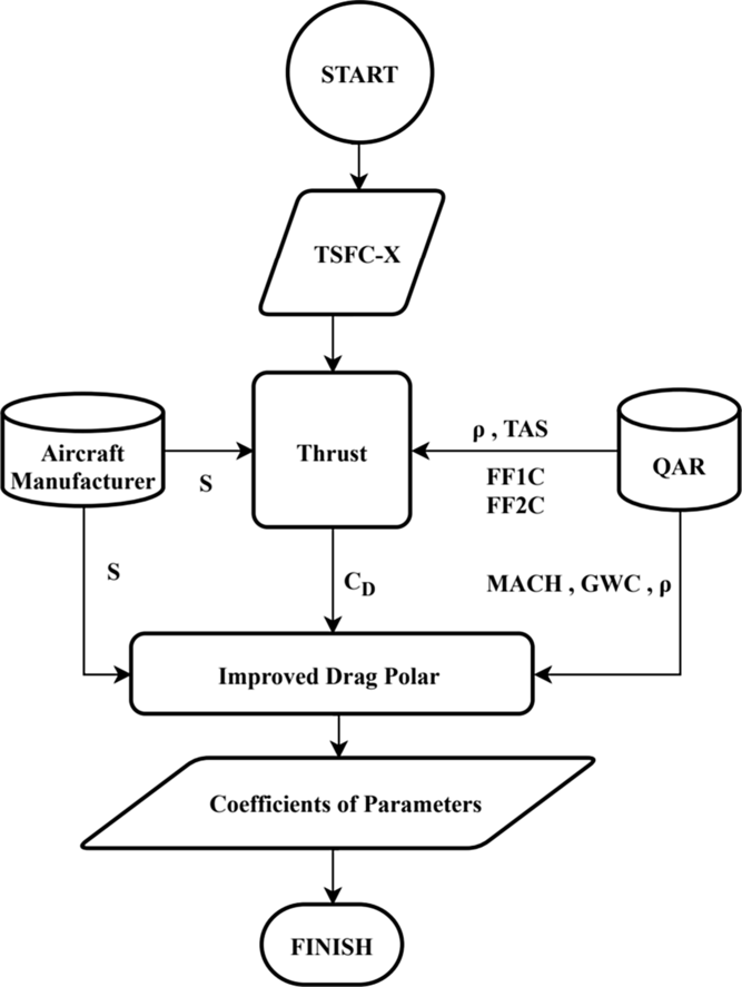
All the flight data were examined and processed in three stages. First, the data were imported from the Excel files. Second, the data were processed, and mathematical models were generated for the drag polar using a code written in MATLAB. Corrupt or missing data were detected and filtered using this code. In the final stage, the processed data were exported to output files in Excel format to perform statistical analysis in MINITAB 19 software and generate tables and figures. The steps of the code used for the estimation of the cruise performance parameters are as follows:

Figure 5. Block diagram for selection between TSFC models (Steps 1–3.1).
Step 1 Determine the cruise flight phase of each flight in the QAR data
Step 2 Identify and classify the aircraft and engine types
Step 3 Generate and calculate the cruise performance model:
Step 3.1 Calculate the thrust-specific fuel consumption values
Step 3.1.1 Calculate the thrust for simple drag polar and an uncambered wing
Step 3.1.2 Calculate the fuel flow rate (FF) for each thrust-specific fuel consumption model
Step 3.1.3 Select the thrust-specific fuel consumption model
Step 3.2 Generate the drag polar model:
Step 3.2.1 Calculate the thrust values using the selected thrust-specific fuel consumption model
Step 3.2.2 Calculate the drag polar values considering the effects of camber and compressibility
Step 3.2.3 Generate the drag model for the lift coefficient and Mach number as independent variables
Step 4 Verify the aerodynamic performance model of the different aircraft and engine type groups
Step 5 Calculate R E (the Breguet cruise range based on the estimated drag and selected TSFC model using the QAR data), R BB (the basic Breguet cruise range based on simple drag polar and the TSFC model from BADA) and R BH (the basic Hale cruise range based on simple drag polar and the TSFC model from BADA).
4.1. Selection of the TSFC model
A flowchart describing Steps 1–3.1 is presented in Fig. 5. The code first checks the flight path angle, altitude, and flight time (FLT_PTH, ALT_STDC and TIME) parameters of each flight to determine the top of climb and top of descent times of the cruise. The code only assigns level flights (with zero flight path angle) at or above 20,000ft as the cruise phase.
Table 6 Performance characteristics of engines


Figure 6. Block diagram for the drag polar model (Step 3.2).
After determining the cruise phases, it is necessary to identify the aircraft and engine types in order to estimate the TSFC values accurately. These data are not available in the QAR data and were thus obtained indirectly using tail codes (TAIL_1) and company tail codes (TAIL_2) from Airfleets(39). Based on this aircraft and engine type groups information, type-specific parameters such as the reference TSFC and Mach numbers (TSFC* and M*), and the bypass ratio (λ) were obtained from manufacturers’ published data. Table 6 presents the reference engine characteristics provided by manufacturers(Reference Roux40). To calculate the thrust-specific fuel consumption values of the cruise flight phase, it is necessary to select thrust-specific fuel consumption models suitable for this flight phase. In Step 3, the code first selects the TSFC that most closely fits the QAR fuel flow rate (FF) data through Steps 3.1.1 to 3.1.3. For each cruise flight phase, three TSFC values are estimated in Step 3.1.1 using the models of Martinez-Val et al.(Reference Martinez-Val and Perez26) (TSFC-1), How et al.(Reference Howe23) (TSFC-2) and Roux(Reference Roux24) (TSFC-3) described in Equations (8)–(10), respectively.
Once the TSFC values have been obtained, thrust values are estimated using level-flight conditions at the given cruise altitude and true airspeed:
 \begin{equation}T = D = \frac{1}{2}\rho {V_{TAS}}^2S{C_D}.\end{equation}
In Equation (14), the air density (ρ) is calculated for the given pressure altitude from the QAR data and the aircraft wing planform area obtained from the aircraft manufacturer. In this step, a simple parabolic drag polar model in Equation (12) is assumed to estimate the thrust (T). After estimating the thrust values, in Step 3.1.2 the fuel flow rate values FF1, FF2 and FF3 are calculated using Equation (7) for TSFC1, TSFC2 and TSFC3, respectively. In Step 3.1.3, the MAPE is estimated for each fuel flow rate with reference to the real fuel flow rate (FFQAR) from the QAR data:
 \begin{equation}MAP{E_i} = \frac{{100}}{N}\mathop \sum \limits_{j=1}^N \left| {\frac{{F{F_{QAR}} - F{F_{ij}}}}{{F{F_{QAR}}}}} \right|\left( {i=1,2,3} \right).\end{equation}
The TSFC resulting in the lowest MAPE in Equation (15)(Reference De Myttenaere, Golden, Le Grand and Rossi41) is selected as the TSFC to be used in the generation of the drag polar model from the QAR data.
4.2 Estimation of the drag polar model
After choosing the appropriate TSFC model (TSFC-X), the next step is the generation of the aerodynamic performance model in Step 3.2. Using Equation (7), the thrust values are calculated for the TSF-X and the real fuel flow rate values for the QAR data. To perform the aerodynamic modelling for the aircraft, the drag polar equation must be formed, taking the effects of the Mach number and cambered wing into account for commercial aircraft. In Step 3.2.1, the drag coefficients (C D) are estimated using the TSFC-X and QAR data, including the fuel flow rate, altitude and true airspeed for each cruise phase. As suggested in Young(Reference Young38), the most appropriate form for the drag polar is a sixth-order polynomial when considering commercial aircraft flying at or above Mach 0.6. Therefore, the drag polar model is formulated as follows:
 \begin{equation}{C_D}\left( {{C_L},M} \right) = {C_{{D_0}}}(M) + \left( {{K_1}(M)} \right){C_L}^2 + \left( {{K_2}(M)} \right){C_L}^6,\end{equation}
In Equation (16), C D0, K 1 and K 2 are expressed as functions of the Mach number based on regression analysis of the QAR data:
 \begin{equation}{C_{D0}}(M) = {a_1} + {a_2}{\left( {M - {M_{Ref}}} \right)^2} + {a_3}{\left( {M - {M_{Ref}}} \right)^3},\end{equation}
 \begin{equation}{K_1}(M) = {b_1} + {b_2}{\left( {M - {M_{Ref}}} \right)^2}\; + {b_3}{\left( {M - {M_{Ref}}} \right)^3} + {b_4}{\left( {M - {M_{Ref}}} \right)^4}, \end{equation}
 \begin{equation}{K_2}(M) = {c_1}\left( {M - {M_{Ref}}} \right) + {c_2}{\left( {M - {M_{Ref}}} \right)^2}.\end{equation}
In Equation (17)–(19), the reference Mach number (MRef) is chosen as 0.6. The coefficients a 1, a 2, a 3, b 1, b 2, b 3, b 4, c 1 and c 2 in the drag polar expression are found by using the nonlinear least-squares method, which is an optimisation model. To check the goodness of fit of the resulting regression model, R 2 values were also calculated. R 2 takes values between 0 and 1. An R 2 value of 1 indicates that the regression model accounts for nearly all of the variability, where R 2 = 0 denotes that the regression model cannot explain the variability(Reference Hagquist and Stenbeck42). Finally, the improved drag polar model is generated using regression analysis between C D, as the dependent variable, and M and C L, as the independent variables. After obtaining the parameters for the drag coefficients, the drag polar model is verified on the different aircraft and engine type groups.
4.3 Evaluation of cruise ranges
In the final step of this study, a range model is proposed to estimate more accurate range values. After the examination of different TSFC models, the TSFC with the minimum MAPE is implemented in the Breguet equation. Moreover, a new high-order polynomial drag polar model is generated and included in the range equation to include the effects of camber and compressibility using real flight data. This enhanced range model is expressed as R E;
 \begin{equation}{R_E} = \frac{{{V_{TAS}}}}{{{\rm{TSFC}}\left( {M,h} \right)}}\frac{{{C_L}}}{{{C_D}\left( {{C_L},\;M} \right)}}\ln \frac{{{W_0}}}{{{W_1}}}.\end{equation}
To evaluate the accuracy of the new range model, two existing range equations are also estimated based on aerodynamic and propulsive data provided by Eurocontrol’s BADA, which is a database used to determine aircraft performance, including more than 300 different types of aircraft. Data in this model are derived from various aircraft documents provided by aircraft manufacturers or operators. It is necessary to point out, however, that the BADA aerodynamic model does not consider the effects of compressibility on the aerodynamic behaviour of the aircraft. Hence, BADA uses a simple parabolic drag model. In BADA, TAS is the only variable affecting the TSFC model(36). The first range equation is referred to as the basic Breguet range equation and is formulated using Equation (21), along with simple drag polar coefficients and the TSFC model from BADA:
 \begin{equation}{R_{BB}} = \frac{{{V_{TAS}}}}{{{\rm{TSFC}}\left( {{V_{TAS}}} \right)}}\frac{{{C_L}}}{{{C_D}\left( {{C_L}} \right)}}\ln \frac{{{W_0}}}{{{W_1}}}.\end{equation}
The second range equation is referred to as the basic Hale range equation, based on linearised constant-altitude and constant-airspeed cruise, in Equation (6):
 \begin{equation}{R_{BH}} \cong 2\frac{{{V_{TAS}}}}{{{\rm{TSFC}}\left( {{V_{TAS}}} \right)}}\frac{1}{{2\sqrt {{C_{D0}}K} }}\left[ {\frac{{{C_{D0}}}}{K}\frac{{\rho {V_{TAS}}^2S}}{{2{W_0}}}\frac{{1 - \frac{{{W_1}}}{{{W_0}}}}}{{\frac{{{C_{D0}}}}{K}{{\left( {\frac{{\rho {V_{TAS}}^2S}}{{2{W_0}}}} \right)}^2} + \frac{{{W_1}}}{{{W_0}}}}}} \right].\end{equation}
In Equation (22), the values of the coefficients C D0 and K of the simple drag model and the TSFC model are also taken from BADA for the considered aircraft and engine type groups.
5.0 RESULTS
The numerical results of the TSFC models, drag polar and range calculations are presented in the following sections.
5.1 TSFC models
The values of the TSFC models are presented in Fig. 7 for all the aircraft and engine type groups in the QAR data. Except for A 2E 2, TSFC-3 based on Roux(Reference Roux24) provides the highest values for all aircraft and engine type groups. The medians of TSFC-1 (Martinez-Val et al.(Reference Martinez-Val and Perez26)) and TSFC-2 (How et al.(Reference Howe23)) are very close to each other for the A 3E 3 and A 6E 6 groups, while those of TSFC-3 are significantly higher. These differences strongly depend on the values of the reference parameters provided by the engine manufacturers (Table 7). For the group A 1E 1, the medians of the TSFC models are relatively closer, while they are almost the same for A 2E 2. The interquartile range of TSFC-2 is narrower than those of TSFC-1 and TSFC-3 for all the groups. Table 7 presents the descriptive statistics for the thrust values estimated using a simple parabolic drag polar equation for each aircraft and engine type group. A comparison of the estimated (FF-1, FF-2 and FF-3) and real fuel flow rates (FFQAR) is shown in Fig. 8. It can be seen that the median of FF-1 is the closest to FFQAR for all the aircraft and engine type groups.
Table 7 Thrust value distribution


Figure 7. Values for the TSFC models for all aircraft and engine type groups.
Table 8 Comparison of the TSFC models


Figure 8. Comparison of the estimated and real fuel flow rates.
Table 8 presents the MAPE results for the FF-1, FF-2 and FF-3 values with respect to FFQAR. The FF-1 values show the lowest MAPE for A 3E 3, A 5E 5 and A 6E 6, while the FF-2 values are slightly better than those of FF-1 for A 1E 1 and A 2E 2. For A 5E 5, they have the same MAPE of 5.6. Rather than choosing different TSFC models for each aircraft and engine type group, we chose TSFC-1, which is the TSFC model with the lowest average MAPE of 8.2 for the fuel flow rate for all the groups.
5.2 Drag polar model
The values of the coefficients of the sixth-order polynomial drag are presented along with the adjusted R 2 values for all the aircraft and engine type groups in Table 9. The adjusted R 2 values range between 0.85 and 0.88. The variation of the drag polar values (C D) obtained according to the C L and Mach number is shown in Figs 9, 10, 11, 12, 13 and 14. As can be seen from these figures, as the C L and Mach number increase, the drag values are more greatly affected. In contrast to low-speed flight, the compressibility effect of air in high-speed flight causes this change.
Table 9 Aerodynamic model coefficients and adjusted R 2 values


Figure 9. C D versus C L and cruise Mach number for A 1E 1.

Figure 10. C D versus C L and cruise Mach number for A 2E 2.
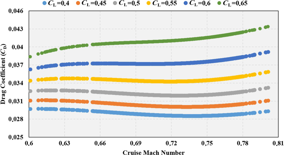
Figure 11. C D versus C L and cruise Mach number for A 3E 3.
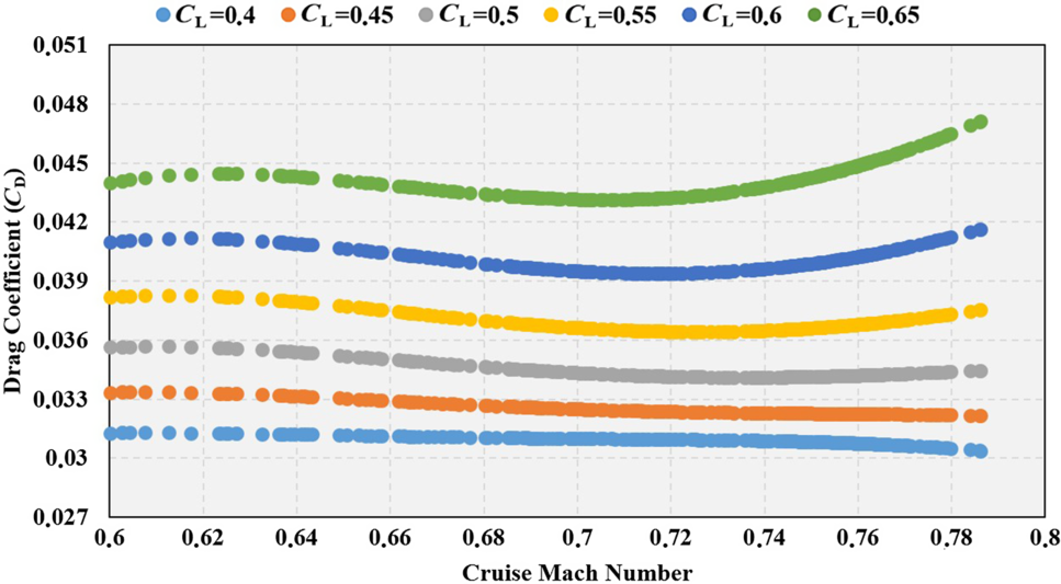
Figure 12. C D versus C L and cruise Mach number for A 4E 4.

Figure 13. C D versus C L and cruise Mach number for A 5E 5.
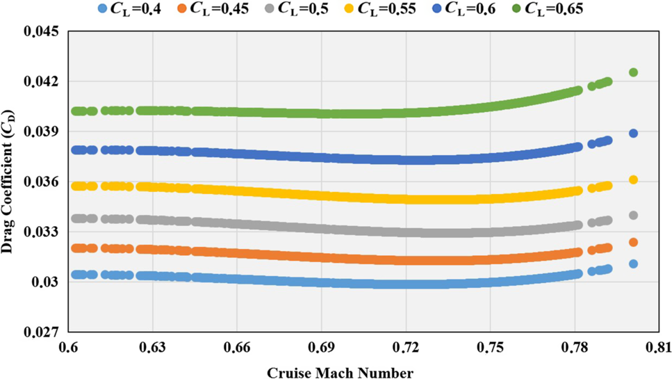
Figure 14. C D versus C L and cruise Mach number for A 6E 6.
5.3 Estimated cruise ranges
A comparison of the real with the calculated range values is presented in Tables 10, 11, 12, 13, 14 and 15. The real range values vary from 59 to 624nm (SD changes between 92 and 116nm). These low values are expected as the sample data were collected from short-distance domestic flights. The mean cruise range for the basic Breguet range values lies between 129 and 240nm (SD changes between 81 and 109nm). When the values of the enhanced range model are examined, it is seen that the mean of the cruise range values lies between 149 and 264nm (SD changes between 92 and 123). As can be seen from these comparisons, the enhanced range model values are closer to the real values than those of the basic Breguet range equation or basic Hale range equation.
Table 10 Comparison of real range values and range calculations for A 1E 1

Table 11 Comparison of real range values and range calculations for A 2E 2

Table 12 Comparison of real range values and range calculations for A 3E 3

Table 13 Comparison of real range values and range calculations for A 4E 4

Table 14 Comparison of real range values and range calculations for A 5E 5

Table 15 Comparison of real range values and range calculations for A 6E 6

The variation of the MAPE values of R E, R BB and R BH with cruise length is presented in Figs 15, 16, 17, 18, 19 and 20. Inspecting all of these figures reveals that the enhanced range equation, R E, has smaller errors than the basic Breguet and basic Hale range equations. Besides, the MAPE distribution of R E improves as the cruise length increases, except for A 2E 2. In the aircraft–engine group A 6E 6, a relatively better result was obtained compared with the basic Breguet or basic Hale range equation results. The reason for this difference is that the engine data from BADA are generic.

Figure 15. The variations of MAPE with range calculations for A 1E 1.

Figure 16. The variations of MAPE with range calculations for A 2E 2.

Figure 17. The variations of MAPE with range calculations for A 3E 3.

Figure 18. The variations of MAPE with range calculations for A 4E 4.

Figure 19. The variations of MAPE with range calculations for A 5E 5.

Figure 20. The variations of MAPE with range calculations for A 6E 6.
The MAPE values were calculated for each aircraft and engine type group according to the real flight data and are presented in Table 16. The MAPE values for the basic Breguet range equation and basic Hale range equation are 7.9% and 8.2%, respectively. When applying the enhanced range model, which is constructed differently from the other range models, the error rate is below 2%, when excluding the A 2E 2 aircraft–engine type. Although A 1E 1 and A 2E 2 are in the same manufacturer’s group (Fig. 3) and have the same airframe type, their MAPE values are significantly different. The reason for the high MAPE values of the A 2E 2 aircraft–engine type is mainly due to the data received from the engine manufacturers, which is needed in the calculation of the TSFC. Engine data are not always shared by engine manufacturers, or shared in their entirety, which can lead to less reliable results. The MAPE values of the aircraft–engine types in group 2 vary between 1.6% to 2.0%. A 3E 3, the aircraft–engine type with the lowest wing loading ratios, has relatively higher MAPE values than the other aircraft–engine types in group 2. Besides A 4E 4 and A 6E 6, the types having a higher thrust-to-weight ratio and wing loading have relatively lower MAPE values.
Table 16 Mean absolute percentage error for range calculations

6.0 DISCUSSION AND CONCLUSION
Aircraft range performance has an impact on economic sustainability as well as having environmental effects. Incorrect calculations of aircraft range performance can result in not only congestion and delays but also economic damage, as well as greater fuel consumption and environmental pollution. Therefore, aircraft range performance, including aircraft aerodynamic performance and engine performance, should be calculated accurately. The range equation proposed herein predicts cruise ranges with significantly lower MAPE values for cruise lengths between 50 and 600nm. QAR data taken from narrow-body aircraft with turbofan engines flying on short-distance domestic subsonic flights were used to improve the cruise range equation. Being able to determine the accurate effects of aircraft performance parameters on the cruise range contributes to the sustainability of aviation. The parameters affecting the cruise range were determined by considering the widely used Breguet range equation. In particular, it was observed that these parameters were the TSFC, representing engine performance, and the drag polar, representing aerodynamic performance. It was found that the effects of the Mach number and wing camber should also be taken into account when constructing the drag polar equations for commercial aircraft and, furthermore, that different TSFC models should be used for each flight phase. It is possible to calculate the TSFC values for the cruise flight phase by correctly selecting the TSFC models.
In conclusion, because modern commercial aircraft have cambered wings and turbofan engines with a high bypass ratio, the use of a constant or simplified TSFC function depending only on the Mach number along with a simple parabolic drag polar is not appropriate for calculations of the cruise range and cruise flight conditions. The analyses performed in this study were limited to commercial narrow-body turbofan aircraft serving short-distance domestic routes. In future studies, data on commercial medium-range body turbofan aircraft making long-range flights could be analyzed and the results compared with those presented herein.
ACKNOWLEDGEMENTS
This study is supported by Eskişehir Technical University Scientific Research Project Commissions under grant number 1708F476. The flight data used in this study were obtained for the research project supported by the Scientific and Technological Research Council of Turkey (TUBITAK) under grant number 111Y048.