


NOMENCLATURE
- Ai
-
surface of a wing strip
- b
-
wing span
- B
-
wing half-span
- C
-
local aerofoil chord
- C di
-
drag coefficient of a wing strip aerofoil
- C li
-
lift coefficient of a wing strip aerofoil
- C D 0
-
wing profile drag coefficient
- CD
-
wing drag coefficient
- CL
-
wing lift coefficient
- Cm
-
wing pitching moment coefficient
- CP
-
pressure coefficient
- ci
-
chord of a wing strip
- c i
-
unit vector in the direction of the local chord for a wing strip
- C(u)
-
point on a NURBS curve
- dF i
-
force vector acting on the bound segment of a horseshoe vortex
- F
-
aerodynamic force generated by the wing
- k
-
turbulent kinetic energy
- dl i
-
vector along the bound segment of a horseshoe vortex
- dM i
-
quarter chord moment of a wing strip
- M
-
aerodynamic moment about the root chord quarter chord point generated by the wing
- N
-
number of horseshoe vortices on the wing surface
- N i, n
-
NURBS curve basis functions
- n i
-
unit vector normal to the wing surface for a wing strip
- p
-
static pressure
- p 0
-
reference pressure
- P i
-
control point of a NURBS curve
- r 0
-
vector along a vortex segment
- r 1
-
vector from the beginning of a vortex segment to an arbitrary point in space
- r 2
-
vector from the end of a vortex segment to an arbitrary point in space
- r i
-
position vector of wing strip quarter chord with reference to root chord quarter chord point
- Re
-
Reynolds number
- Reθt
-
momentum thickness transition Reynolds number
- S
-
wing area
- ti
-
NURBS curve knot
- u
-
NURBS curve parameter
- v ∞
-
unit vector in the direction of the freestream
- v i, j
-
velocity induced by horseshoe vortex j, considered to be of unit intensity, at the control point of horseshoe vortex i
- V
-
velocity vector
- V ∞
-
freestream velocity vector
- V i
-
local velocity at the bound segment of a horseshoe vortex
- wi
-
NURBS curve weights
- X
-
chord-wise coordinate
- Y
-
span-wise coordinate
- α i
-
local angle-of-attack for a wing strip
- γ
-
intermittency
- Γ
-
vortex intensity
- Δyi
-
span of a wing strip
- ρ
-
air density
- μ
-
dynamic viscosity
- μ t
-
turbulent viscosity
-
 $\bar \tau $
-
stress tensor
- ω
-
specific dissipation rate

1.0 INTRODUCTION
One of the major research efforts of the present day aerospace industry is concentrated on reducing fuel consumption and making aircrafts more efficient. Flight tests have demonstrated that a 20% reduction in aircraft drag could lead to an 18% reduction in fuel consumption(Reference Okamoto and Rhee1). The active modification of the wing shape, for purposes such as promoting a larger laminar flow region on the wing surface, could lead to a substantial drag reduction(Reference Zingg, Diosady and Billing2). The main advantage of actively modifying the wing shape using a morphing technique is that an optimal shape for the wing and/or aerofoil can be provided during each distinct phase of aircraft flight, for each of the various airflow conditions. In addition to achieving important reductions in fuel consumption, adaptive, morphing wings can also be effectively used to replace conventional high-lift devices(Reference Pecora, Barbarino, Concilio, Lecce and Russo3-Reference Diodati, Concilio, Ricci, De Gaspari, Liauzun and Godard5), or the conventional control surfaces(Reference Pecora, Amoroso and Lecce6).
In recent years, the development and application of morphing solutions on Unmanned Aerial Vehicles (UAVs) has garnered considerable interest, due to the increasingly greater efficiency requirements and their much simpler certification issues, compared to manned aircrafts. Various researchers have presented concepts for morphing UAVs that achieved performance improvements over the traditional, fixed geometry versions. Neal et al(Reference Neal, Good, Johnston, Robertshaw, Mason and Inman7) and Supekar(Reference Supekar8) used telescopic pneumatic actuators to change the UAV wing planform and achieve an increase in the lift-to-drag ratio over the entire flight envelope. Gamboa et al(Reference Gamboa, Alexio, Vale, Lau and Suleman9) designed a UAV wing capable of independent span and chord changes that achieved drag reductions of up to 23% when compared to the non-morphing geometries.
Gano and Renaud(Reference Gano and Renaud10) presented a concept to increase the aerodynamic efficiency of a UAV by gradually decreasing the wing thickness as the fuel inside the wing-mounted tank was consumed, while Shyy et al(Reference Shyy, Jenkins and Smith11) presented research on small UAV aerofoils that passively morphed in response to changes in external aerodynamic forces. Do Vale et al(Reference do Vale, Leite, Lau and Suleman12) developed a morphing wing capable of span changes through a telescopic system, but in addition achieved conformal changes of its aerofoil camber. The two morphing mechanisms could independently change the wing shape, and were designed for a UAV application, by using a coupled aerodynamic-structural optimisation process. Falcao et al(Reference Falcao, Gomes and Suleman13) proposed a new design of a morphing winglet for a military class UAV. By changing the winglet cant and toe angles, the system could achieve important performance improvements by effectively controlling the lift distribution at the wingtip region according to different flight conditions. Previtali et al(Reference Previtali, Arrieta and Ermanni14) performed numerical studies to investigate the roll control performance of a morphing wing concept that used compliant ribs and that were aimed to replace the conventional ailerons.
Bartley-Cho et al(Reference Bartley-Cho, Wang, Martin, Kudva and West15) presented a variable camber wing, actuated by piezoelectric motors and integrated into a Northrop-Grumman combat UAV. Bilgen et al(Reference Bilgen, Kochersberger, Diggs, Kurdila and Inman16,Reference Bilgen, Kochersberger and Inman17) designed and tested a concept of replacing the ailerons with local, continuous wing camber changes. In addition to the academic environment, aircraft manufacturing companies have also shown interest in the development of next-generation morphing UAVs. Lockheed Martin's Agile Hunter UAV concept(Reference Bye and McClure18-Reference Love, Zink, Stroud, Bye, Rizk and White20) was developed into a wind-tunnel prototype capable of folding the inner wing sections over the fuselage to reduce the drag during transonic cruise. NextGen Aeronautic created the MFX1 UAV prototype(Reference Andersen, Cowan and Piatak21,Reference Flanagan, Strutzenberg, Myers and Rodrian22) , with variable wing sweep and wing area, and demonstrated its significant in-flight planform-changing capabilities in several successful flight tests.
The objective of the CRIAQ 7.1 project was to improve and control the laminarity of the flow past a morphing wing wind-tunnel model in order to obtain important drag reductions(Reference Botez, Molaret and Laurendeau23). The wing was equipped with a flexible composite material upper surface whose shape could be changed using internally placed shape memory alloy (SMA) actuators(Reference Brailovski, Terriault, Coutu, Georges, Morellon, Fischer and Berube24). The numerical study revealed very promising results: the morphing system was able to delay the transition location downstream by up to 30% of the chord and reduce the aerofoil drag by up to 22%(Reference Pages, Trifu and Paraschivoiu25). The actuator optimal displacements for each of the flight conditions were provided using both a direct open-loop approach(Reference Popov, Grigorie, Botez, Mamou and Mébarki26,Reference Grigorie, Popov and Botez27) and a closed-loop configuration based on real time pressure readings from the wing upper surface(Reference Popov, Grigorie, Botez, Mamou and Mébarki28,Reference Popov, Grigorie, Botez, Mamou and Mébarki29) . In addition, a new controller based on an optimal combination of the bi-positional and PI laws was developed(Reference Grigorie, Popov, Botez, Mamou and Mébarki30,Reference Grigorie, Popov, Botez, Mamou and Mébarki31) . The wind-tunnel tests were performed in the 2×3m atmospheric closed-circuit subsonic wind tunnel at IAR-NRC, and validated the numerical wing optimisations(Reference Sainmont, Paraschivoiu, Coutu, Brailovski, Laurendeau, Mamou and Khalid32) and the designed control techniques(Reference Grigorie, Botez and Popov33-Reference Grigorie and Botez36).
2.0 MORPHING WING CONCEPT
The actual implementation of a wing surface morphing technique on the real Hydra Technologies UAS-S4 requires that only a limited portion of the entire wing surface is allowed to change, and that the modifications are small enough to be feasible from structural and control points of view. Thus, all the numerical optimisations were performed with regard to the technological possibilities and constraints required by the practical implementation of the morphing wing concept. Only a limited part of the UAS's conventional rigid wing skin was replaced using a flexible skin whose shape can be modified using actuators placed inside the wing structure. Figure 1 presents a chord-wise section through the wing, identifying the morphing and the rigid parts of the wing skin (left), and shows a top view of the wing, with the span-wise limits of the morphing skin (right).

Figure 1. Chord-wise section through the morphing wing (left) and topside view of the morphing skin (right).
The morphing skin replaces a part of the wing's rigid upper surface. In the chord-wise direction, the skin starts close to the leading edge at x/c = 0.01 and extends on the upper surface up to x/c = 0.55, where c represents the local chord of the wing aerofoil. The ending point of the flexible skin is limited by the presence of the wing control surfaces such as the flaps and the ailerons. The attachment between the rigid and flexible portions is made in a way that ensures continuity and a smooth transition between the two regions. In the span-wise direction, the morphing skin starts close to the UAV wing/fuselage junction, at y/b = 0.19 and extends to the wing tip, at y/b = 0.98, where b represents the wing half-span, as measured from the fuselage centreline up to the wing tip.
In order to provide the required deformations of the morphing skin, the internal actuators are arranged into a number of chord-wise actuation lines, each line consisting of several actuators placed at a desired y/b span-wise position. For the purpose of the numerical analysis, the wing span-wise sections that correspond to the actuation lines are parameterised using non-uniform rational b-splines (NURBS)(Reference Piegl and Tiller37,Reference Farin38) . The NURBS are a generalisation of B-Splines and Bézier curves, being defined by their order, a polygon of weighted control points and a knot vector, and making use of the de Boor recursive formula(Reference de Boor39) to calculate the values of the basis functions:
 $$\begin{equation}
\begin{array}{l} {{\bf C}}\left( u \right) = \mathop \sum \limits_{i = 1}^k \frac{{{N_{i,n}}{w_i}}}{{\mathop \sum \nolimits_{j = 1}^k {N_{j,n}}{w_j}}}{{{\bf P}}_i}\\[12pt] {N_{i,1}} = \left\{ {\begin{array}{*{20}{c}} {1,\ \ if\ {t_i} \le u \le {t_{i + 1}}}\\[3pt] {0,\ \ otherwise\ \ \ \ \ \ \ \ \ \ } \end{array}} \right.\\[12pt] {N_{i,n}} = \frac{{u - {t_i}}}{{{t_{i + n}} - {t_i}}}{N_{i,n - 1}} + \frac{{{t_{i + n + 1}} - u}}{{{t_{i + n + 1}} - {t_i}}}{N_{i + 1,n - 1}} \end{array}
\end{equation}$$
$$\begin{equation}
\begin{array}{l} {{\bf C}}\left( u \right) = \mathop \sum \limits_{i = 1}^k \frac{{{N_{i,n}}{w_i}}}{{\mathop \sum \nolimits_{j = 1}^k {N_{j,n}}{w_j}}}{{{\bf P}}_i}\\[12pt] {N_{i,1}} = \left\{ {\begin{array}{*{20}{c}} {1,\ \ if\ {t_i} \le u \le {t_{i + 1}}}\\[3pt] {0,\ \ otherwise\ \ \ \ \ \ \ \ \ \ } \end{array}} \right.\\[12pt] {N_{i,n}} = \frac{{u - {t_i}}}{{{t_{i + n}} - {t_i}}}{N_{i,n - 1}} + \frac{{{t_{i + n + 1}} - u}}{{{t_{i + n + 1}} - {t_i}}}{N_{i + 1,n - 1}} \end{array}
\end{equation}$$
In Equation (1), u is the curve parameter, ranging from 0 (the start of the curve) to 1 (the end of the curve), k is the number of control points, n is the order of the curve, wi are the weights associated with the control points, ti are the knots, N i, n are the basis functions and P i = [xi,yi,zi ] are the control points.
In the numerical optimisation, the change of the morphing skin shape is achieved by changing the coordinates of the NURBS control points, a motion that is strictly controlled. For each span-wise actuation line and for each control point of that line, a vector that passes through the control point and that is normal to the local aerofoil curve is calculated. The motion of the control points is then restricted to the direction given by this vector. In addition, the control points cannot move for more than a given length along this direction so as to maintain the deformations of the flexible skin within acceptable predefined limits. Figure 2 shows the NURBS control points that correspond to one span-wise section of the wing (left), and also presents the direction of motion and the limits imposed on one of the control points (right).

Figure 2. Control points for one span-wise section (left) and the movement constraints for one selected point (right).
3.0 WING PERFORMANCE CALCULATION METHODOLOGY
The aerodynamic performance of the wing is calculated using a three-dimensional numerical extension of the classical lifting-line method, in which two-dimensional aerodynamic data from several span-wise wing sections is integrated into the three-dimensional global mathematical model to determine the wing aerodynamic characteristics(Reference Sugar Gabor, Koreanschi and Botez40,Reference Sugar Gabor, Koreanschi and Botez41) . The method follows the methodology proposed by Phillips and Snyder(Reference Phillips and Snyder42).
3.1 Nonlinear lifting line method
The continuous distributions of bound vorticity over the wing surface and of trailing vorticity in the wing wake are approximated using a finite number of horseshoe vortices. The bound segment of the vortices is aligned with the wing quarter chord line, while the trailing segments are aligned with the direction of the freestream as presented in Fig. 3.

Figure 3. Horseshoe vortices distribution over the wing surface (taken from(Reference Phillips and Snyder42)).
The velocity induced by a straight vortex segment at an arbitrary point in space, such as any of the three segments making a horseshoe vortex, is given by the Biot-Savart formula(Reference Phillips and Snyder42,Reference Katz and Plotkin43) :
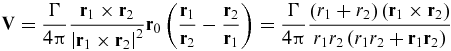 $$\begin{equation}
{{\bf V}} = \frac{\Gamma }{{4\pi }}\frac{{{{{\bf r}}_1} \times {{{\bf r}}_2}}}{{{{\left| {{{{\bf r}}_1} \times {{{\bf r}}_2}} \right|}^2}}}{{{\bf r}}_0}\left( {\frac{{{{{\bf r}}_1}}}{{{{{\bf r}}_2}}} - \frac{{{{{\bf r}}_2}}}{{{{{\bf r}}_1}}}} \right) = \frac{\Gamma }{{4\pi }}\frac{{\left( {{r_1} + {r_2}} \right)\left( {{{{\bf r}}_1} \times {{{\bf r}}_2}} \right)}}{{{r_1}{r_2}\left( {{r_1}{r_2} + {{{\bf r}}_1}{{{\bf r}}_2}} \right)}}
\end{equation}$$
$$\begin{equation}
{{\bf V}} = \frac{\Gamma }{{4\pi }}\frac{{{{{\bf r}}_1} \times {{{\bf r}}_2}}}{{{{\left| {{{{\bf r}}_1} \times {{{\bf r}}_2}} \right|}^2}}}{{{\bf r}}_0}\left( {\frac{{{{{\bf r}}_1}}}{{{{{\bf r}}_2}}} - \frac{{{{{\bf r}}_2}}}{{{{{\bf r}}_1}}}} \right) = \frac{\Gamma }{{4\pi }}\frac{{\left( {{r_1} + {r_2}} \right)\left( {{{{\bf r}}_1} \times {{{\bf r}}_2}} \right)}}{{{r_1}{r_2}\left( {{r_1}{r_2} + {{{\bf r}}_1}{{{\bf r}}_2}} \right)}}
\end{equation}$$
In Equation (2), Γ is the vortex intensity, r 1 and r 2 are the spatial vectors from the starting and ending points of the vortex segment to the arbitrary point in space, r 1 and r 2 are the moduli of the spatial vectors, and r 0 is the spatial vector along the length of the vortex segment.
Each horseshoe vortex is made up of three straight vortex lines; one of them is bound to the wing quarter chord line and the other two are aligned with the freestream velocity. The typical geometry of a horseshoe vortex is presented in Fig. 4.

Figure 4. Geometry details for a typical horseshoe vector.
By applying Equation (2) on all of the segments of the horseshoe vortex and summing the obtained velocities, the velocity induced at an arbitrary point in space can be determined:
 $$\begin{equation}
{{\bf V}} = \frac{\Gamma }{{4\pi }}\frac{{{{{\bf v}}_\infty } \times {{{\bf r}}_2}}}{{{r_2}\left( {{r_2} - {{{\bf v}}_\infty }{{{\bf r}}_2}} \right)}} + \frac{\Gamma }{{4\pi }}\frac{{\left( {{r_1} + {r_2}} \right)\left( {{{{\bf r}}_1} \times {{{\bf r}}_2}} \right)}}{{{r_1}{r_2}\left( {{r_1}{r_2} + {{{\bf r}}_1}{{{\bf r}}_2}} \right)}} - \frac{\Gamma }{{4\pi }}\frac{{{{{\bf v}}_\infty } \times {{{\bf r}}_1}}}{{{r_1}\left( {{r_1} - {{{\bf v}}_\infty }{{{\bf r}}_1}} \right)}}
\end{equation}$$
$$\begin{equation}
{{\bf V}} = \frac{\Gamma }{{4\pi }}\frac{{{{{\bf v}}_\infty } \times {{{\bf r}}_2}}}{{{r_2}\left( {{r_2} - {{{\bf v}}_\infty }{{{\bf r}}_2}} \right)}} + \frac{\Gamma }{{4\pi }}\frac{{\left( {{r_1} + {r_2}} \right)\left( {{{{\bf r}}_1} \times {{{\bf r}}_2}} \right)}}{{{r_1}{r_2}\left( {{r_1}{r_2} + {{{\bf r}}_1}{{{\bf r}}_2}} \right)}} - \frac{\Gamma }{{4\pi }}\frac{{{{{\bf v}}_\infty } \times {{{\bf r}}_1}}}{{{r_1}\left( {{r_1} - {{{\bf v}}_\infty }{{{\bf r}}_1}} \right)}}
\end{equation}$$
The continuous distribution of vorticity over the wing surface and in the wing wake is approximated with N horseshoe vortices, each vortex having its own intensity Γ i . To determine the unknown values of the vortex intensities, the three-dimensional vortex lifting law(Reference Phillips and Snyder42,Reference Katz and Plotkin43) is applied to express the inviscid force dF i acting on the bound segment of each horseshoe vortex:
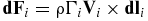 $$\begin{equation}
{{\bf d}}{{{\bf F}}_i} = \rho {\Gamma _i}{{{\bf V}}_i} \times {{\bf d}}{{{\bf l}}_i}
\end{equation}$$
$$\begin{equation}
{{\bf d}}{{{\bf F}}_i} = \rho {\Gamma _i}{{{\bf V}}_i} \times {{\bf d}}{{{\bf l}}_i}
\end{equation}$$
In Equation (4), dF i is the local force acting on a differential segment of the lifting line, a segment that is identical to the bound segment of the horseshoe vortex with an intensity of Γ i , ρ is the fluid density, V i is the local airspeed vector, and dl i is the spatial vector along the lifting line differential segment, aligned according to the local vorticity. The local airspeed vector over one bound vortex segment is equal to the sum of the freestream velocity V ∞ and the velocities induced by all the other horseshoe vortices distributed over the wing surface and wake:
 $$\begin{equation}
{{{\bf V}}_i} = {{{\bf V}}_\infty } + \mathop \sum \limits_{j = 1}^N {\Gamma _j}{{{\bf v}}_{ij}}
\end{equation}$$
$$\begin{equation}
{{{\bf V}}_i} = {{{\bf V}}_\infty } + \mathop \sum \limits_{j = 1}^N {\Gamma _j}{{{\bf v}}_{ij}}
\end{equation}$$
In the above Equation (5), v ij is the velocity induced at the bound segment of horseshoe vortex i by the unit strength horseshoe vortex j and is given by Equation (3), in which the vortex intensity is considered to be Γ = 1.
From classical wing theory, the magnitude of the inviscid force acting on a wing strip of area Ai and having a local aerofoil lift coefficient C li is given by Equation (6):
 $$\begin{equation}
\left\| {{{{\bf F}}_i}} \right\| = \frac{1}{2}\rho V_\infty ^2{A_i}{C_{{l_i}}}
\end{equation}$$
$$\begin{equation}
\left\| {{{{\bf F}}_i}} \right\| = \frac{1}{2}\rho V_\infty ^2{A_i}{C_{{l_i}}}
\end{equation}$$
The local aerofoil lift coefficient can be determined using other means, such as experimentally determined lift curves or 2D simulations using fast, coupled panel methods/boundary-layer codes, provided that the local strip angle-of-attack is known. This local angle-of-attack α i can be calculated using the local strip velocity V i , the local aerofoil chord-wise unit vector c i and the unit vector normal to the local aerofoil chord n i , and is given by Equation (7):
 $$\begin{equation}
{ \propto _i} = {\tan ^{ - 1}}\left( {\frac{{{{{\bf V}}_i}{{{\bf n}}_i}}}{{{{{\bf V}}_i}{{{\bf c}}_i}}}} \right)
\end{equation}$$
$$\begin{equation}
{ \propto _i} = {\tan ^{ - 1}}\left( {\frac{{{{{\bf V}}_i}{{{\bf n}}_i}}}{{{{{\bf V}}_i}{{{\bf c}}_i}}}} \right)
\end{equation}$$
If the wing strips are taken such that each horseshoe vortex-bound segment corresponds to one strip, then the modulus of the force given by Equation (4) can be set equal to the one given by Equation (6), since the bound segment is the only segment upon which the surrounding fluid exerts a force, the trailing segments being aligned with the freestream. Thus, for each vortex over the wing surface, the following equation can be written:
 $$\begin{equation}
\left\| {\rho {\Gamma _i}\left( {{{{\bf V}}_\infty } + \mathop \sum \limits_{j = 1}^N {\Gamma _j}{{{\bf v}}_{ij}}} \right) \times {{\bf d}}{{{\bf l}}_i}} \right\| - \frac{1}{2}\rho V_\infty ^2{A_i}{C_{{l_i}}} = 0,\ \ \ i = 1,2, \ldots ,N
\end{equation}$$
$$\begin{equation}
\left\| {\rho {\Gamma _i}\left( {{{{\bf V}}_\infty } + \mathop \sum \limits_{j = 1}^N {\Gamma _j}{{{\bf v}}_{ij}}} \right) \times {{\bf d}}{{{\bf l}}_i}} \right\| - \frac{1}{2}\rho V_\infty ^2{A_i}{C_{{l_i}}} = 0,\ \ \ i = 1,2, \ldots ,N
\end{equation}$$
The non-linear system of equations obtained by combining the N equations written for each horseshoe vortex can be solved using Newton's classical method for nonlinear systems to provide the unknown vortex intensities. Once all of the horseshoe vortices’ intensities have been calculated, the aerodynamic force and moment about the root chord quarter chord point can be determined, using Equations (9) and (10):
 $$\begin{equation}
{{\bf F}} = \rho \mathop \sum \limits_{i = 1}^N \left[ {\left( {{{{\bf V}}_\infty } + \mathop \sum \limits_{j = 1}^N {\Gamma _j}{{{\bf v}}_{ij}}} \right){\Gamma _i} \times {{\bf d}}{{{\bf l}}_i}} \right]\\
\end{equation}$$
$$\begin{equation}
{{\bf F}} = \rho \mathop \sum \limits_{i = 1}^N \left[ {\left( {{{{\bf V}}_\infty } + \mathop \sum \limits_{j = 1}^N {\Gamma _j}{{{\bf v}}_{ij}}} \right){\Gamma _i} \times {{\bf d}}{{{\bf l}}_i}} \right]\\
\end{equation}$$
 $$\begin{equation}
{{\bf M}} = \rho \mathop \sum \limits_{i = 1}^N {{{\bf r}}_i} \times \left[ {\left( {{{{\bf V}}_\infty } + \mathop \sum \limits_{j = 1}^N {\Gamma _j}{{{\bf v}}_{ij}}} \right){\Gamma _i} \times {{\bf d}}{{{\bf l}}_i}} \right] + {{\bf d}}{{{\bf M}}_i}
\end{equation}$$
$$\begin{equation}
{{\bf M}} = \rho \mathop \sum \limits_{i = 1}^N {{{\bf r}}_i} \times \left[ {\left( {{{{\bf V}}_\infty } + \mathop \sum \limits_{j = 1}^N {\Gamma _j}{{{\bf v}}_{ij}}} \right){\Gamma _i} \times {{\bf d}}{{{\bf l}}_i}} \right] + {{\bf d}}{{{\bf M}}_i}
\end{equation}$$
The great advantage of this method is that it can provide the wing viscous drag in addition to the inviscid wing characteristics, since the calculated span-wise vorticity distribution has been constrained not only by the lifting line hypothesis but also by the local aerofoil characteristics, which have been determined taking into consideration the fluid viscosity effects. In addition, if the strip aerofoil shapes are changed by the morphing technique, then the effects of this deformation on the wing performance are automatically determined. The wing viscous drag coefficient is given by Equation (11):
 $$\begin{equation}
{C_{{D_0}}} = \frac{1}{S}\mathop \int \limits_{ - b/2}^{b/2} {C_d}\left( y \right)c\left( y \right)dy \cong \frac{1}{S}\mathop \sum \limits_{i = 1}^N {C_{{d_i}}}{c_i}\Delta {y_i}
\end{equation}$$
$$\begin{equation}
{C_{{D_0}}} = \frac{1}{S}\mathop \int \limits_{ - b/2}^{b/2} {C_d}\left( y \right)c\left( y \right)dy \cong \frac{1}{S}\mathop \sum \limits_{i = 1}^N {C_{{d_i}}}{c_i}\Delta {y_i}
\end{equation}$$
Here, S represents the wing area, b is the wingspan, C di is the local aerofoil drag coefficient calculated together with the local lift coefficient C li , ci represents the local wing chord and Δyi is the span of the local wing strip.
3.2 Calculation of the strip aerofoil aerodynamic properties
The 2D aerofoil calculations are performed using the XFOIL code(Reference Drela and Youngren45). The inviscid estimation of the velocity field over the aerofoil surface is done using a linear vorticity stream function panel method(Reference Drela46). The boundary-layer properties are determined with a two-equation, lagged dissipation integral boundary-layer formulation(Reference Drela47), incorporating a modified, implicit version of the eN laminar-to-turbulent transition criterion(Reference Drela48). The boundary layer and the wake flow interact with the inviscid potential flow by means of the surface transpiration model, and the two sets of equations are solved simultaneously using Newton's method for nonlinear systems.
4.0 THE OPTIMISATION APPROACH
For each different flight condition, the optimal displacements of the morphing wing internal actuators are determined using an original, in-house-developed optimisation code(Reference Sugar Gabor, Koreanschi and Botez49) based on a coupling of the Artificial Bee Colony (ABC) algorithm with the Broyden-Fletcher-Goldfarb-Shano (BFGS) algorithm, and using the numerical lifting line methodology for estimating the morphed-wing aerodynamic performance.
The ABC algorithm is an optimisation algorithm based on the intelligent behaviour of a honeybee swarm. Karaboga and Basturk(Reference Karaboga and Basturk50) conceived the original algorithm in 2007, and it was applicable only to the unconstrained optimisation of linear and nonlinear problems. Other authors have proposed methods for enhancing the algorithm's capabilities, such as the handling of constrained optimisation problems(Reference Karaboga and Basturk51) or the significant improvement of its convergence properties(Reference Zhu and Kwong52). Because the ABC algorithm simultaneously performs a global search throughout the entire definition domain of the objective function and a local search around the more promising solutions already found, it can efficiently avoid converging towards a local minimum point of the objective function, and thus is able to approximate the global optimum point.
Once the region of the global optimum has been found, the algorithm's rate of convergence decreases and the local search routine of the ABC method is replaced by the Broyden-Fletcher-Goldfarb-Shanno (BFGS) algorithm(Reference Bonnans, Gilbert, Lemarechal and Sagastizabal53), a type of quasi-Newtonian iterative method for nonlinear optimisation problems. Since the BFGS method can only be applied to unconstrained optimisation, it was coupled with the Augmented Lagrangian Method (ALM)(Reference Powell54) to introduce the desired optimisation constraints. Using the ALM-BFGS approach allows for a significantly faster determination of the global optimum position, thus accelerating the convergence rate of the final steps of the optimisation procedure. The details of the ABC and BFGS algorithms are presented in Fig. 5, as well as the general configuration of the morphing wing optimisation procedure.

Figure 5. Details of the morphing wing optimisation procedure.
5.0 VALIDATION OF RESULTS WITH HIGH-FIDELITY DATA
In order to validate the morphing wing results obtained with the numerical lifting line model, the calculations were also performed using the state-of-the-art ANSYS FLUENT(55) flow solver, with advanced turbulent flow modelling and incorporating a laminar-to-turbulent transition criterion to provide accurate drag force estimations. The external flow around the wing is governed by the classical fluid dynamics equations for the conservation of mass and of momentum:
 $$\begin{equation}
\displaystyle\frac{{\partial \rho }}{{\partial t}} + \nabla \times \left( {\rho {{\bf V}}} \right) = 0\\
\end{equation}$$
$$\begin{equation}
\displaystyle\frac{{\partial \rho }}{{\partial t}} + \nabla \times \left( {\rho {{\bf V}}} \right) = 0\\
\end{equation}$$
 $$\begin{equation}
\displaystyle\frac{\partial }{{\partial t}}\left( {\rho {{\bf V}}} \right) + \nabla \times \left( {\rho {{\bf VV}}} \right) = - \nabla p + \nabla \times \bar \tau
\end{equation}$$
$$\begin{equation}
\displaystyle\frac{\partial }{{\partial t}}\left( {\rho {{\bf V}}} \right) + \nabla \times \left( {\rho {{\bf VV}}} \right) = - \nabla p + \nabla \times \bar \tau
\end{equation}$$
In Equations (12) and (13), ρ is the fluid density, V is the velocity vector, p is the static pressure and
 $\bar \tau $
is the stress tensor, given by the following expression:
$\bar \tau $
is the stress tensor, given by the following expression:
 $$\begin{equation}
\bar \tau = \mu \left[ {\left( {\nabla {{\bf V}} + \nabla {{{\bf V}}^T}} \right) - \frac{2}{3}\nabla \times {{\bf V}}\bar I} \right]
\end{equation}$$
$$\begin{equation}
\bar \tau = \mu \left[ {\left( {\nabla {{\bf V}} + \nabla {{{\bf V}}^T}} \right) - \frac{2}{3}\nabla \times {{\bf V}}\bar I} \right]
\end{equation}$$
Here, μ is the fluid dynamic viscosity and
 $\bar I$
is the unit tensor. The turbulent nature of the flow is modelled using the Reynolds-Averaged Navier-Stokes (RANS) approach and the Boussinesq hypothesis for modelling the Reynolds stresses. The mathematical model closure and the calculation of the turbulent viscosity μ
t
are done with the k − ω Shear-Stress Transport (SST) turbulence model(Reference Menter56). The k − ω SST model consists of two equations, one for the turbulent kinetic energy k and one for the specific dissipation rate ω:
$\bar I$
is the unit tensor. The turbulent nature of the flow is modelled using the Reynolds-Averaged Navier-Stokes (RANS) approach and the Boussinesq hypothesis for modelling the Reynolds stresses. The mathematical model closure and the calculation of the turbulent viscosity μ
t
are done with the k − ω Shear-Stress Transport (SST) turbulence model(Reference Menter56). The k − ω SST model consists of two equations, one for the turbulent kinetic energy k and one for the specific dissipation rate ω:
 $$\begin{equation}
\displaystyle\frac{\partial }{{\partial t}}\left( {\rho k} \right) + \frac{\partial }{{\partial {x_i}}}\left( {\rho k{u_i}} \right) = \frac{\partial }{{\partial {x_j}}}\left( {{\Gamma _k}\frac{{\partial k}}{{\partial {x_j}}}} \right) + {G_k} - {Y_k}\\
\end{equation}$$
$$\begin{equation}
\displaystyle\frac{\partial }{{\partial t}}\left( {\rho k} \right) + \frac{\partial }{{\partial {x_i}}}\left( {\rho k{u_i}} \right) = \frac{\partial }{{\partial {x_j}}}\left( {{\Gamma _k}\frac{{\partial k}}{{\partial {x_j}}}} \right) + {G_k} - {Y_k}\\
\end{equation}$$
 $$\begin{equation}
\displaystyle\frac{\partial }{{\partial t}}\left( {\rho \omega } \right) + \frac{\partial }{{\partial {x_i}}}\left( {\rho \omega {u_i}} \right) = \frac{\partial }{{\partial {x_j}}}\left( {{\Gamma _\omega }\frac{{\partial \omega }}{{\partial {x_j}}}} \right) + {G_\omega } - {Y_\omega } + {D_\omega }
\end{equation}$$
$$\begin{equation}
\displaystyle\frac{\partial }{{\partial t}}\left( {\rho \omega } \right) + \frac{\partial }{{\partial {x_i}}}\left( {\rho \omega {u_i}} \right) = \frac{\partial }{{\partial {x_j}}}\left( {{\Gamma _\omega }\frac{{\partial \omega }}{{\partial {x_j}}}} \right) + {G_\omega } - {Y_\omega } + {D_\omega }
\end{equation}$$
In these equations, ui are the components of the velocity vector, Gk represents the production of turbulent kinetic energy, G ω represents the production of ω, Γ k and Γω are the effective diffusivities of k and ω, Yk and Y ω represent the dissipation of k and ω due to turbulence itself, and D ω represents the cross-diffusion term.
In order to include the effects of laminar flow over the wing surface, and thus accurately determine the laminar-to-turbulent transition region, the k − ω SST turbulence model has been coupled with the γ − Re θ transition model(Reference Menter, Langtry, Likki, Suzen, Huang and Volker57). The model uses two equations, one for the intermittency γ and one for the transition onset criteria in terms of the momentum thickness transition Reynolds number Reθt :
 $$\begin{equation}
\displaystyle\frac{\partial }{{\partial t}}\left( {\rho \gamma } \right) + \frac{\partial }{{\partial {x_i}}}\left( {\rho \gamma {u_i}} \right) = \frac{\partial }{{\partial {x_j}}}\left[ {\left( {\mu + \frac{{{\mu _t}}}{{{\sigma _\gamma }}}} \right)\frac{{\partial \gamma }}{{\partial {x_j}}}} \right] + {P_{\gamma 1}} - {E_{\gamma 1}} + {P_{\gamma 2}} - {E_{\gamma 2}}\\
\end{equation}$$
$$\begin{equation}
\displaystyle\frac{\partial }{{\partial t}}\left( {\rho \gamma } \right) + \frac{\partial }{{\partial {x_i}}}\left( {\rho \gamma {u_i}} \right) = \frac{\partial }{{\partial {x_j}}}\left[ {\left( {\mu + \frac{{{\mu _t}}}{{{\sigma _\gamma }}}} \right)\frac{{\partial \gamma }}{{\partial {x_j}}}} \right] + {P_{\gamma 1}} - {E_{\gamma 1}} + {P_{\gamma 2}} - {E_{\gamma 2}}\\
\end{equation}$$
 $$\begin{equation}
\displaystyle\frac{\partial }{{\partial t}}\left( {\rho {\rm{R}}{{\rm{e}}_{\theta t}}} \right) + \frac{\partial }{{\partial {x_i}}}\left( {\rho {\rm{R}}{{\rm{e}}_{\theta t}}{u_i}} \right) = \frac{\partial }{{\partial {x_j}}}\left[ {{\sigma _{\theta t}}\left( {\mu + {\mu _t}} \right)\frac{{\partial {\rm{R}}{{\rm{e}}_{\theta t}}}}{{\partial {x_j}}}} \right] + {P_{\theta t}}
\end{equation}$$
$$\begin{equation}
\displaystyle\frac{\partial }{{\partial t}}\left( {\rho {\rm{R}}{{\rm{e}}_{\theta t}}} \right) + \frac{\partial }{{\partial {x_i}}}\left( {\rho {\rm{R}}{{\rm{e}}_{\theta t}}{u_i}} \right) = \frac{\partial }{{\partial {x_j}}}\left[ {{\sigma _{\theta t}}\left( {\mu + {\mu _t}} \right)\frac{{\partial {\rm{R}}{{\rm{e}}_{\theta t}}}}{{\partial {x_j}}}} \right] + {P_{\theta t}}
\end{equation}$$
In Equations (17) and (18), P γ1 and E γ1 are the transition source terms, P γ2 and E γ2 are the destruction/relaminarisation source terms, P θt is the transition momentum thickness Reynolds number source term, and σγ and σθt are the model constants.
In the numerical simulation, the steady-state flow equations are solved using a projection method, achieving the constraint of mass conservation by solving a pressure equation. The cell-face values of the velocity and of the turbulence variables are calculated with the third-order MUSCL (Monotone Upstream-Centred Scheme for Conservation Laws) scheme, while the cell-face values of the pressure are estimated using a second-order central-differencing interpolation scheme. The discrete equations are solved in a fully implicit coupled manner using an Algebraic Multi-Grid (AMG) approach for providing significant convergence acceleration and the block-method Incomplete Lower-Upper (ILU) decomposition algorithm as the linear system smoother.
6.0 RESULTS AND ANALYSIS
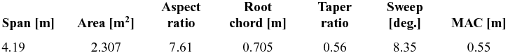
The morphing concept is used to improve the aerodynamic characteristics of the Hydra Technologies UAS-S4 Éhecatl wing. This UAS was designed and build in Mexico and serves as a state-of-the-art aerial surveillance system for both military and civilian missions. The geometrical characteristics of the UAS-S4 wing are presented in Table 1.
Table 1 Geometric characteristics of the UAS-S4 wing
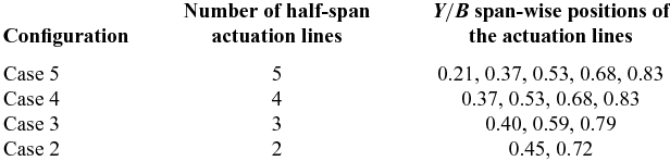
In the chord-wise direction, the morphing skin stretches between x/c = 0.01 and x/c = 0.55, where c represents the local chord of the wing, while in the span-wise direction, the morphing skin extends between y/b = 0.19 and y/b = 0.98 where b represents the wing half-span as measured from the fuselage centreline up to the wing tip. In order to analyse the influence of modifying the upper surface shape on the wing aerodynamic characteristics, four different configurations were proposed for the number and positions of the chord-wise actuation lines. Table 2 presents the details of these four configurations. For convenience and to make reading the results easier, the configurations are named according to the number of actuation lines.
Table 2 Details of the four actuation lines’ configurations
For each configuration, only the wing cross-section aerofoils corresponding to the actuation lines span-wise positions are parameterised using NURBS and are directly modified in the optimisation procedure. Thus, the actuator displacements for any actuation line are simulated by changing the coordinates of the NURBS control points corresponding to that wing cross-section aerofoil. The shape of the morphing wing surface between two consecutive actuation lines is determined by performing cubic splines interpolations in the span-wise direction. Figure 6 presents the Case 3 configuration of the morphing wing, where the span-wise positions of the three actuation lines and the limits of the morphing skin in the figure were not kept exact, for the purpose of better visualisation. The blue outline represents the flexible upper skin, while the three wing cross-sections (A, B and C) represent the actuation lines where the local aerofoil shapes can be directly optimised. The original aerofoil is the same for all three cross-sections, but the morphed aerofoil of each section can vary as a function of the optimisation procedure results.

Figure 6. The modification of the upper surface morphing skin shape control using three span-wise actuation lines.
The optimisation is focused on improving the wing lift-to-drag ratio L/D over a rage of angle-of-attack values. The analyses were performed at an airspeed of 50m/s, with a Reynolds number of Re = 2.133 × 10⁶, as calculated with the mean aerodynamic chord. The reference values for air density, pressure and molecular viscosity are those of standard atmosphere at sea level (ρ = 1.225kg/m3, p 0 = 101, 000Pa, μ = 1.79*10−5 Pa · s). The turbulence intensity level was set to 0.07%, corresponding to calm atmospheric conditions. Detailed results showing the influence of the morphing upper skin on the performance of the UAS wing are presented for four angle-of-attack values.
Figure 7 presents a comparison of the span-wise variations of the local lift coefficient CL, the local induced drag coefficient CDI and the local profile drag coefficient CD0 for a wing angle-of-attack of –2°.

Figure 7. Span-wise variation of lift, induced drag and profile drag coefficients at an angle-of-attack of –2°.
A comparison of the pressure coefficient distributions for two span-wise wing sections, y = 1m (left) and y = 1.8m (right), at a wing angle-of-attack of –2°, is presented in Fig. 8.

Figure 8. Pressure coefficient distributions for y = 1.0 (left) and y = 1.8 (right) sections at an angle-of-attack of –2°.
Figure 9 presents a comparison of the span-wise variations of the local lift coefficient CL, the local induced drag coefficient CDI and the local profile drag coefficient CD0 for a wing angle-of-attack of 1°.

Figure 9. Span-wise variation of lift, induced drag and profile drag coefficients at an angle-of-attack of 1°.
A comparison of the pressure coefficient distributions for two span-wise wing sections, y = 1m (left) and y = 1.8m (right), at a wing angle-of-attack of 1°, is presented in Fig. 10.

Figure 10. Pressure coefficient distributions for y = 1.0 (left) and y = 1.8 (right) sections at an angle-of-attack of 1°.
Figure 11 presents a comparison of the span-wise variations of the local lift coefficient CL, the local induced drag coefficient CDI and the local profile drag coefficient CD0 for a wing angle-of-attack of 4°.
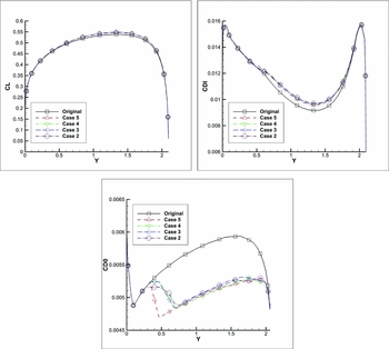
Figure 11. Span-wise variation of lift, induced drag and profile drag coefficients at an angle-of-attack of 4°.
A comparison of the pressure coefficient distributions for two span-wise wing sections, y = 1m (left) and y = 1.8m (right), at a wing angle-of-attack of 4°, is presented in Fig. 12.

Figure 12. Pressure coefficient distributions for y = 1.0 (left) and y = 1.8 (right) sections at an angle-of-attack of 4°.
Figure 13 presents a comparison of the span-wise variations of the local lift coefficient CL, the local induced drag coefficient CDI and the local profile drag coefficient CD0 for a wing angle-of-attack of 8°.

Figure 13. Span-wise variation of lift, induced drag and profile drag coefficients at an angle-of-attack of 8°.
A comparison of the pressure coefficient distributions for two span-wise wing sections, y = 1m (left) and y = 1.8m (right), at a wing angle-of-attack of 8°, is presented in Fig. 14.

Figure 14. Pressure coefficient distributions for y = 1.0 (left) and y = 1.8 (right) sections at an angle-of-attack of 8°.
Concerning the impact on the span-wise distribution of lift and induced drag, it can be seen that all four proposed configurations give approximately the same results. From the angles of attack chosen for the detailed comparisons, the highest increase in span-wise lift is obtained for an angle-of-attack of 4°, as seen from Fig. 11.
The reduction of the span-wise profile drag coefficient is significant for all angles of attack, achieving increasingly higher performance as the angle-of-attack increases. The configuration with five actuator lines per wing semi-span obtains the most important reductions, but the gains over the other three configurations are not very large. The sudden drop in profile drag observed for Case 5 is attributed to the small distance between the flexible skin limit and the first actuation line. This drop cannot be observed for the other three configurations, as they present a smoother transition between the rigid and the flexible regions.
The analysis of the pressure coefficient distributions shows that the flexible skin reduces the adverse pressure gradient for the leading-edge region of the wing, leading to a smoother pressure increase and thus increasing the lift. Again, the differences between the four proposed morphing wing configurations are relatively small and all of them successfully achieve the desired effects.
Table 3 presents a comparison between the CL/CD ratio for the original wing and for each of the four different configurations of the morphing wing. At each angle-of-attack value, the improvement percentage is indicated, in addition to the CL/CD numeric values.
Table 3 Results of CL/CD optimisation at all considered angle-of-attack values

An improvement of the lift-to-drag ratio of the morphing wing over the original wing was obtained for the entire range of angles of attack. All four configuration cases achieve the best improvements for the angle-of-attack interval between 2° and 4°, corresponding to the region of maximum lift-to-drag of the original wing. The five actuation lines per semi-span case consistently obtained the best performance increase.
The verification of the results obtained with the lifting-line method was performed with the ANSYS FLUENT solver. Two configurations were chosen for the comparison: the one with the highest number of span-wise actuation lines (Case 5) and the one with the lowest number of span-wise actuation lines (Case 2). The 3D single-block structured H-Type meshes around the original and morphed wing geometries were generated with the ANSYS ICEM-CFD grid generator. The normal distance for the wall cells was set to 2.0 × 10⁻⁶m, while the far-field boundaries were placed 50 chords away from the wing. The calculations were performed at an airspeed of 50m/s, with a Reynolds number of Re = 2.133 × 10⁶, as calculated with the mean aerodynamic chord, and at two angle-of-attack values: 1° and 4°. Figure 15 shows a cut out of the 3D mesh around the wing and Fig. 16 presents an example of typical residual convergence curves. For all the calculations, the converged residuals were in the range of 10−5 to 10−10, achieved within 500-550 AMG cycles.

Figure 15. Cut of the UAS-S4 H-Type structured mesh.

Figure 16. Typical residual convergence curves.
A comparison between the lift coefficient, the drag coefficient, the pitching moment coefficient and the lift-to-drag ratio for the original wing and the two configurations chosen (Cases 2 and 5) for the validation is presented in Table 4. The 3D results obtained with FLUENT are compared to those obtained with the nonlinear lifting line method coupled with the 2D section viscous data.
Table 4 Comparison of aerodynamic coefficients obtained with the in-house code and FLUENT

It can be observed, for the comparisons between the original and morphed wings, that the performance improvements obtained with the optimisation procedure and the rapid lifting line code are also present in the results obtained using the high-fidelity CFD solver. These results show that the lifting line code can be used for wing optimisation procedures, as it provides sufficiently accurate wing performance information, and it can predict whether the modified geometry outperforms the original geometry with respect to the desired optimisation goal.
The detailed RANS results show that the drag reductions observed in Table 4 can be attributed to the larger extent of laminar flow on the upper surface of the morphed geometries. Figures 17 and 18 present the surface plot of the turbulent kinetic energy for the original wing and the Case 5 morphed wing. It can be seen that for the morphed geometries, the onset of turbulent flow is significantly delayed towards the trailing edge.

Figure 17. Plot of turbulent kinetic energy on the upper surface on the original wing (left) and the Case 5 morphed wing (right) at an angle-of-attack of 1°.

Figure 18. Plot of turbulent kinetic energy on the upper surface on the original wing (left) and the Case 5 morphed wing (right) at an angle-of-attack of 4°.
A comparison between the pressure coefficient distributions obtained with the in-house nonlinear lifting line code (NLL) and those obtained with FLUENT is presented next. Figure 19 shows the comparison at a 1° angle-of-attack for the y = 1m section, while Fig. 20 presents the comparison at the same angle-of-attack for the y = 1.8m section. In Figs. 21 and 22, the pressure coefficient comparisons are made for the same span-wise stations, but for an angle-of-attack of 4°.

Figure 19. Pressure coefficient distributions for y = 1.0 sections at an angle-of-attack of 1°.

Figure 20. Pressure coefficient distributions for y = 1.8 sections at an angle-of-attack of 1°.

Figure 21. Pressure coefficient distributions for y = 1.0 sections at an angle-of-attack of 4°.

Figure 22. Pressure coefficient distributions for y = 1.8 sections at an angle-of-attack of 4°.
7.0 CONCLUSIONS
The aerodynamic performance of the Hydra Technologies UAS-S4 wing was improved using a numerical morphing wing optimisation approach. The shape of the wing upper surface was modified as function of the flight condition with the goal of increasing the lift-to-drag ratio compared to the baseline design. In the numerical optimisations, the wing cross-sections were parameterised using non-uniform rational b-splines, and the upper surface displacements were achieved by moving the spline curves control points along predetermined directions. Four possible configurations were proposed, as function of different number of actuation lines placed on each half-span of the wing.
For each different flight condition defined by a given Reynolds number, airspeed and angle-of-attack, the optimal displacements were determined with an optimisation code based on a coupling of the Artificial Bee Colony and the Broyden-Fletcher-Goldfarb-Shanno algorithms. The aerodynamic qualities of each morphed wing geometry were calculated using a rapid, nonlinear lifting line method, coupled with a two-dimensional viscous flow solver. For validation purposes, several selected wing geometries were also calculated using a high-fidelity Navier-Stokes solver. The results proved that the lifting line code could successfully be used for the optimisation routine, as this code provides accurate wing performance information.
The wing optimisations were performed at a fixed airspeed within the UAS-S4 flight envelope, for an angle-of-attack range between –4 and 8°, with the objective function of increasing the lift-to-drag ratio. All four proposed actuation configurations significantly reduced the profile drag over the entire span of the flexible skin for the complete range of angles of attack. The configuration using the highest number of span-wise actuation lines achieved the best results, allowing morphing wing lift-to-drag ratio to increase up to 4% compared to the original geometry.
8.0 FUTURE WORK
In order to reproduce the numerically calculated optimised shapes, a part of the UAS-S4 upper surface will be replaced by a flexible, composite material skin whose shape can be modified using internally placed actuators. A material suitable for achieving the desired skin displacements must be chosen. Based on the errors between the aerodynamic target shapes and the finite element model calculated shapes, several configurations will be analysed: a) keeping the morphing skin as an active structural component of the UAS wing or b) redesigning the spars and ribs so that the skin can be freed from the loads induced by wing bending and torsion. An internal actuation system must be designed that is capable of providing the desired displacements while remaining constrained by the available internal space and position of spars and ribs. Once the skin material and the final wing structure are established, an energy consumption analysis of the morphing system under combined aerodynamic and structural forces will be performed, thus quantifying the overall power consumption gains of the concept.
ACKNOWLEDGEMENTS
We would like to thank the Hydra Technologies Team in Mexico for their continuous support, and especially Mr. Carlos Ruiz, Mr. Eduardo Yakin and Mr. Alvaro Gutierrez Prado. We would also like to thank to the Natural Sciences and Engineering Research Council of Canada (NSERC) for the funding of the Canada Research Chair in Aircraft Modelling and Simulation Technologies. In addition, we would like to thank to the Canada Foundation of Innovation (CFI), to the Ministère du Développement Économique, de l'Innovation et de l'Exportation (MDEIE), and to Hydra Technologies for the acquisition of the UAS-S4 using the Leaders Opportunity Funds.


