NOMENCLATURE

Acronyms

AAIB

Air Accidents Investigation Branch

CAA

Civil Aviation Authority

CAP437

CAA publication CAP437

CFD

Computational Fluid Dynamics

CoG

Centre of Gravity

CoP

Centre of Pressure

DP

Dynamic Positioning

ERF

European Rotorcraft Forum

FDR

Flight Data Recorder

FPSO

Floating Production Storage and Offloading

FRASCA

FRASCA International Inc

HCA

Helideck Certification Agency

HMS

Helideck Monitoring System

HSRMC

Helicopter Safety Research Management Committee

kgf

kilogram force (${\rm kg\cdot g}$)

MMS

Measure of Motion Severity

MPOG

Minimum Pitch on Ground

MRU

Motion Reference Unit

MSI

Motion Severity Index

MWS

Measure of Wind Severity

NASA

National Aeronautics and Space Administration

OEM

Original Equipment Manufacturer

RFM

Rotorcraft Flight Manual

ROS

Reserve of Stability

RWD

Relative Wind Direction

WSI

Wind Severity Index

UK

United Kingdom

Symbols

$\vec{a}$

total acceleration, inertial and gravitational

a_h

acceleration in the plane of the helideck

a_x

acceleration in x-direction

a_y

acceleration in y-direction

a_z

acceleration normal to the helideck

A, A_side, A_front

fuselage cross-sectional areas

C_d

drag coefficient

CGX

longitudinal CoG distance relative to point N

CGY

lateral CoG distance from centre line

CGZ

vertical CoG distance above the helideck surface

exp

based on experimental measurements

F

force

f

force factor

F_CX

longitudinal main rotor control force

F_CY

lateral main rotor control force

F_G

gravitational and inertial force component

f_grav

gravitational term constant

f_i

force factor

f_m

moment factor

F_R

vertical reaction force (total, or measured at each of the N, P or S contact points)

FR

distance between front (nose) and main undercarriage axis mid-point

F_w

wind drag force

FZT

total vertical reaction force

k_w

wind drag constant of proportionality

L

distance between N and P (or S) points

LIFT

main rotor lift force

L_U, L_α, R₀, R₁, U_L

empirical constants for main rotor lift force calculation

LY

half the distance between P and S

m

helicopter mass

M

moments

M_D

destabilising moments

mod

based on modelled values

M_R

restoring moments

N

nose wheel contact point

O_f

orientation factor

O_fTIP

orientation factor for tipping failure

P

port wheel contact point

R

main rotor lift force

ROS_SLIDE

Reserve of Stability for sliding failure

ROS_TIP

Reserve of Stability for tipping failure

R_w

non-dimensional wind drag ratio

S

starboard wheel contact point

U

wind speed

U_L

empirical constants for main rotor lift force calculation

x

longitudinal direction, along helicopter axis of symmetry

y

lateral direction

z

vertical direction

α_s

main rotor disc vertical angle of attack relative to oncoming wind

β

wind direction relative to the helicopter longitudinal axis

γ

in-built main rotor axis inclination relative to helicopter vertical axis

θ

main rotor collective pitch angle

θ_h

orientation angle

θ_u

updraft angle

μ

coefficient of friction of helideck surface

ρ

density of air

2.0 FACTORS AFFECTING ON-DECK STABILITY

The first step in modelling the on-deck ROS of a helicopter has been to consider the factors affecting on-deck stability for all possible modes of failure.

On-deck stability refers to the period of time after a helicopter has touched down and before it takes off. It does not consider risks associated with the initial phase of the landing onto the helideck, i.e. those associated with the touchdown. Touchdown risks are important but different in nature, requiring a fundamentally different approach to assessing and managing them; for this reason, they have been kept separate from the scope of this research programme.

While on deck, an unconstrained helicopter on a moving helideck is susceptible to losing stability either by tipping (or rolling) over onto its side, or by sliding across the deck. It is possible in principle to calculate the point at which stability is lost by calculating all of the forces and moments acting on the helicopter and by using the equilibrium equations in six degrees of freedom.

The reaction forces at each of the helicopter contact points with the helideck (assumed to be the three wheels of a tricycle undercarriage, not skids) can also be calculated from the equilibrium equations and used as a failure criterion. Tipping failure occurs when the vertical reaction at any of the wheels falls to zero. Sliding failure occurs when the horizontal forces exceed the maximum frictional forces that can be generated between the contact points, which in turn are a function of the vertical reactions at the wheels and the coefficient of friction relating to the interface between the helicopter wheels and the helideck surface.

The forces and moments acting on the helicopter will depend on: a) the environmental conditions on the helideck, mainly the helideck motion and ambient wind; b) the helicopter itself, in terms of its design (e.g. helicopter mass and dimensions) and the aerodynamic forces generated by the main and tail rotors, as well as the fuselage drag forces.

Although it might appear relatively straightforward for a helicopter OEM or a technical consultancy to build a model to calculate these forces and moments and then calculate the point of failure by plugging them into the equilibrium equations (e.g. by using existing simulation models and integrating them with available software tools such as FlightLab), there are a number of significant difficulties and limitations associated with this approach.

The first issue is characterising the time-varying and six-dimensional helideck motion (three displacements and three rotations), based on measurements taken in-service on a moving offshore helideck. Currently, the reported deck motion parameters are the 20-minute maxima of roll, pitch, inclination and heave amplitude/heave rate of the helideck, for which limits are set based on in-service experience to regulate operations. These measures do not fully represent the time-variation nor the six-dimensionality of the helideck motion, e.g. they do not capture the dynamic effect of helideck accelerations in all directions. However, it would be impractical to require pilots to absorb and process too many parameters prior to landing. For this reason, the CAA stipulated that the destabilising effect of the helideck should ideally be expressed in terms of a single consolidated parameter, namely the MMS.

Another aspect that became evident during the research was that the forces generated by the wind form another important destabilising factor, that is not adequately covered by the current operational limits which are based on helideck motion alone. The only wind-related operational limit is an upper wind limit set at 60kts, related to the risk of personnel on the helideck being blown overboard. However, as has been demonstrated by the research and in-service incidents, helicopter stability can become compromised at much lower wind speeds, even when the helideck is stationary (e.g. for fixed helidecks). For this reason, a further parameter had to be defined to describe the severity of the wind conditions at a helideck, namely the Measure of Wind Severity (MWS).

In addition to deriving the most representative physical parameters for the MMS and MWS, it was also necessary to develop a modelling approach that would allow these parameters to be linked to the point of failure for all tipping and sliding failure modes. It is possible to calculate the minimum MMS required for failure for a given set of wind conditions and other helicopter parameters by iteratively calculating the forces and moments that could be generated for all possible combinations of deck motion parameters of roll, pitch, and accelerations. However, this is not only inefficient in terms of the computing resources required, but also does not provide much direct insight into:

• the relative contribution of all the destabilising factors.

• the sensitivity of the results to each of the input parameters.

• which helideck motion and wind parameters best correlate with a helicopter’s ‘reserve of stability’ and therefore which parameters should be used to predict helicopter on-deck stability prior to landing.

The desired outcome for the CAA was a model that would provide these insights to enable informed decisions to be made on how best to define and set appropriate limiting criteria for the MMS and MWS. The model therefore had to be:

• as transparent as possible, setting out all assumptions clearly.

• customisable to cover all the different helicopter types operating in the North Sea and to cover all realistic operational scenarios.

• fast to run, allowing the whole range of real-life operational scenarios to be assessed.

• accessible to stakeholders — open-source, not proprietary to any of the helicopter OEMs.

• backed by experimental evidence and best available data.

• amenable to independent checking and continuous improvement.

This paper describes the solution to this very challenging research remit, which has been achieved via the following main steps:

1. a) defining a ROS that can be linked analytically (i.e. in the form of deterministic equations) to any forces and moments acting on a helicopter.

2. b) developing a simple, yet effective, quasi-static analytical model for calculating each of the forces and moments generated by the helideck motion and wind conditions.

3. c) selecting the most representative formulations for the MMS and MWS and linking them directly to the ROS.

3.0 DEFINING THE RESERVE OF ON-DECK STABILITY (ROS)

This section explains how the ROS has been defined, and how it has been linked analytically to the forces and moments acting on a helicopter. It covers all modes of on-deck failure for a nose wheel tricycle undercarriage helicopter, since this represents the type most commonly used for UK offshore operations.

The following main external forces act on a helicopter on a moving helideck:

• helicopter weight (i.e. gravitational force).

• inertial forces acting on the helicopter due to helideck acceleration.

• fuselage wind drag forces.

• main rotor lift.

• main rotor torque.

• control forces — main rotor forces due to cyclic control inputs, and the tail rotor force.

Loss of equilibrium occurs when the total moment of the external forces listed above can no longer be balanced by, a) the moments of the helideck reaction forces acting normal to the helideck, and b) the moments of the frictional forces acting in the plane of the helideck to resist motion. These correspond to the two main modes of failure of tipping and sliding, each of which can occur in a number of ways, as illustrated in Fig. 1.

Figure 1. Illustration of on-deck tipping (about NS, NP and PS axes) and sliding failure modes (using rotation about N as an example).

A helicopter can roll over onto its side by rotating about two possible tipping axes, NP or NS (the axes connecting the nose wheel (N) and either of the main wheels (starboardside (S) or portside (P)). Tipping can also occur relative to the PS axis, i.e. by the lifting of the nose wheel, although this is unlikely to occur in practice for a helicopter with an undercarriage that is typically longer than it is wide.

Sliding can occur in translation or in rotation. A rotational slide is more likely since only two of the wheels have to move instead of all three. Which two wheels will slide first will depend on the balance of moments. Thus, each sliding scenario (about pivot points N, P or S) has to be considered in turn.

For each of the modes of failure identified above, the ROS can be defined by reference to the balance of moments about the rotation axis for each failure mode. For tipping failure this is the NS or NP axis, and for rotational sliding modes it is a rotation relative to the axis normal to the helideck relative to each wheel, clockwise or anti-clockwise.

The ROS has been defined based on the ratio of destabilising, M_D, versus restoring, M_R, moments:

(1)\begin{align}{\rm{ROS}} = 1 - \frac{{( - {M_D})}}{{{M_R}}}\end{align}

This is equal to zero at the point of failure and equal to 1 (100%) when no destabilising forces act on the helicopter.

For tipping failure, the net gravitational plus inertial forces acting normal and downwards onto the helideck always act to restore equilibrium and thus the denominator is assumed equal to the moment of these forces. This restoring moment is due to the ‘effective weight’ of the helicopter (as discussed later) and does not depend on any of the other external forces (assuming that the inertial accelerations are due to helideck motion only and the oleos do not deform significantly).

All other forces, i.e. the total moment of the gravitational and inertial forces acting parallel to the helideck plus that of all other external forces (due to wind drag and rotor forces) are grouped into the destabilising moments, M_D. When the sign of the total M_D is in a destabilising direction, i.e. opposite to that of the restoring moments M_R, its effect is to reduce the ROS. However, the forces in the destabilising grouping could, either individually or even in total, be in a restoring direction, giving a ROS > 1. For example, when considering failure relative to the NS axis in the +ve (anti-clockwise) direction, a force acting on the helicopter towards starboard will generate a moment with a sign opposite to the restoring moment generated by the weight of the helicopter, and the ROS will be <1. However, a force in the opposite direction, will reinforce the restoring moment, giving a ROS >1. The opposite applies to moments for a failure relative to the NP axis which requires a rotation in the -ve direction.

For sliding failure, the only forces consistently acting to restore equilibrium are the frictional forces. The restoring moment is therefore that of the frictional forces, relative to an axis normal to the helideck. All other external forces are grouped under the total destabilising moment. To maintain equilibrium, the frictional restoring moment will adapt to always balance the destabilising moment of the external forces. In order to have a meaningful definition for the ROS, the maximum value of the frictional restoring moment is used in the denominator. This is simply the moment due to each of the frictional forces assuming the maximum value of µ F_R, where µ is the helideck coefficient of friction and F_R is the reaction force on each wheel. However, the reaction force on each wheel does depend implicitly on all other forces acting on the helicopter.

4.0 ANALYTICAL EXPRESSIONS FOR TIPPING AND SLIDING ROS

Using the definition above in Equation (1) the ROS can be linked to each of the forces/moments acting on a helicopter via relatively simple analytical expressions.

The expressions calculated below are particularly useful since they:

1. a) clarify the destabilising effect of helideck motion, representing it in the simplest and most physically insightful way, as a function of the fewest, most fundamental parameters. This has allowed the MMS and other relevant helideck motion parameters to be defined.

2. b) provide a general framework for quantifying how close a helicopter is to tipping or sliding, for any helideck motion, provided that all other external forces generated by the helicopter rotors and generated by the wind can be quantified.

4.1 Tipping failure (NS, NP axes only)

As discussed above, tipping can occur relative to roll-over axes NS, NP, or with the lifting of the nose wheel relative to axis PS. The latter tipping mode is unlikely, however, and is not included in the discussion that follows even though expressions have been derived for this mode of failure also.

The expressions for the NS and NP tipping modes are mathematically symmetrical relative to the longitudinal (x-axis) of the helicopter, given the symmetry of a tricycle helicopter undercarriage. Therefore, the expression presented here for the NS failure mode can easily be adapted for the NP axis. In a stability calculation, both modes will have to be considered; the relative balance of ROS for each mode will depend on the relative directions of the external forces acting on the helicopter, most of which will vary continually while the helicopter is on-deck.

4.1.1 Destabilising effect of helideck motion only

Consider first a helicopter on a moving helideck with no other forces acting on it other than gravitational and inertial forces. The total external force acting on the helicopter is then equal to $m{\kern1pt\cdot\kern1pt}\overrightarrow a $, where $\overrightarrow a $ is the total acceleration of the helideck (gravitational and inertial).

This force can be resolved normal to the helideck and parallel to the helideck. The component acting normal to the helideck, $\textrm{m}{\kern1pt\cdot\kern1pt}a_{z}$, provides a restoring moment, and the component parallel to the helideck, $\textrm{m}{\kern1pt\cdot\kern1pt}a_{h}$, provides a destabilising moment.

Figure 2 illustrates the right-handed coordinate system used throughout, defined with the z axis pointing downwards and normal to the helideck. The x- and y-directions are defined relative to the three helicopter contact points (y-axis parallel to PS).

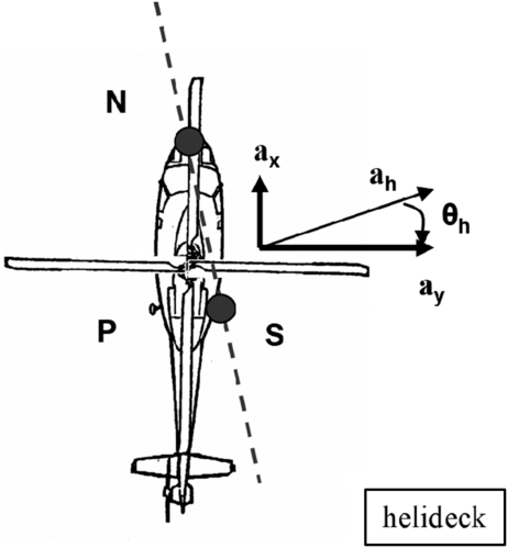
Figure 2. Definition of the orientation factor angle $\uptheta_{\rm h}$, and resultant horizontal acceleration, a_h.

As shown in Fig. 2, a_h is the resultant of the helideck acceleration components a_x and a_y. The angle of a_h relative to the lateral axis of the helicopter is the “orientation angle”, $\uptheta_{\rm h}$, defined as:

(2)\begin{align}\tan {\theta _h} = \frac{{{a_x}}}{{{a_y}}}\end{align}

Using the definition in Equation (1), the ROS for tipping relative to axis NS (ROS_TIP) due to the effect of helideck motion only is equal to:

(3)\begin{align}RO{S_{TIP}} = 1 - \frac{{{\rm{destabilising}}\,{\rm{moment}}\,{\rm{of}}\,m{\kern1pt\cdot\kern1pt}{a_h}}}{{{\rm{restoring}}\,{\rm{moment}}\,{\rm{of}}\,m{\kern1pt\cdot\kern1pt}{a_z}}}\end{align}

It can be shown that this is equal to:

(4)\begin{align}1 - \left( {\frac{{FR}}{L}{\kern1pt\cdot\kern1pt}\cos {\theta _h} + \frac{{LY}}{L}{\kern1pt\cdot\kern1pt}\sin {\theta _h}} \right){\kern1pt\cdot\kern1pt}\frac{{{a_h}}}{{{a_z}}}{\kern1pt\cdot\kern1pt}\frac{{{\rm{CGZ}}}}{{{\rm{CGX}}{\kern1pt\cdot\kern1pt}\frac{{LY}}{L} - {\rm{CGY}}{\kern1pt\cdot\kern1pt}\frac{{FR}}{L}}}\end{align}

where CGX is the longitudinal distance of the centre of gravity (CoG) from the nose wheel of the helicopter, CGY is the lateral offset of the CoG relative to the helicopter centreline, CGZ is the height of the CoG above the helideck. FR is the perpendicular distance between the nose wheel and a line joining the main wheels, LY is half the distance between the main wheels, and L is the distance between the nose wheel contact point, and that of either of the two main wheels.

Thus, the destabilising effect of the helideck motion depends on: a) the ratio of a_h/a_z; b) the orientation angle, $\uptheta_{\rm h}$; c) the location of the CoG; d) the dimensions of the helicopter’s undercarriage.

The ratio a_h/a_z is the single, most representative factor of the destabilising effect of helideck motion, and therefore has been chosen as the measure of helideck motion severity (MMS).

The orientation angle $\uptheta_{\rm h}$ is not purely helideck-dependent since it depends on the orientation of the helicopter relative to the helideck at the time of landing. It is helpful to consider the following grouping, called the orientation factor (O_f):

(5)\begin{align}{O_{{\rm{fTIP}}}} = \frac{{FR}}{L}{\kern1pt\cdot\kern1pt}\cos {\theta _h} + \frac{{LY}}{L}{\kern1pt\cdot\kern1pt}\sin {\theta _h}\end{align}

This multiplies the destabilising effect of the MMS and represents the effect of helicopter orientation on the helideck. O_f is maximum when a_h is oriented normal to the (NS or NP) tipping axes of the helicopter, and zero when a_h is parallel to either of the tipping axes NP or NS. Its maximum value is equal to:

(6)\begin{align}{O_{{\rm{fTIPmax}}}} = \sqrt {{{\left( {\frac{{FR}}{L}} \right)}^2}+{{\left( {\frac{{LY}}{L}} \right)}^2}} = 1\end{align}

Therefore, the reduction of the ROS of a helicopter due to the effect of helideck motion only, can be quantified simply in the general form:

(7)\begin{align}{\rm{RO}}{{\rm{S}}_{{\rm{TIP}}}} = 1 - {\rm{MMS}}{\kern1pt\cdot\kern1pt}{{\rm{O}}_{{\rm{fTIP}}}}({\theta _h}){\kern1pt\cdot\kern1pt}{f_{{\rm{grav}}}}\end{align}

where f_grav is a purely geometrical term, equal to:

(8)\begin{align}{f_{{\rm{grav}}}} = \frac{1}{{\frac{{{\rm{CGX}}}}{{{\rm{CGZ}}}}{\kern1pt\cdot\kern1pt}\frac{{{\rm{LY}}}}{{\rm{L}}} - \frac{{{\rm{CGY}}}}{{{\rm{CGZ}}}}{\kern1pt\cdot\kern1pt}\frac{{{\rm{FR}}}}{{\rm{L}}}}}\end{align}

The same result applies to the NP tipping mode but using the opposite sign for the CGY term, and the opposite sign for the angle $\uptheta_{\rm h}$ in O_fTIP.

4.1.2 Destabilising effect of all other forces

Considering the effect of all other forces, F, and pure moments, M, it can be shown that ROS_TIP can be expressed in the following general form:

(9)\begin{align}{\rm{RO}}{{\rm{S}}_{{\rm{TIP}}}} = 1 - {\rm{MMS}}{\kern1pt\cdot\kern1pt}{{\rm{O}}_{{\rm{fTIP}}}}({\theta _h}){\kern1pt\cdot\kern1pt}{f_{{\rm{grav}}}} - \sum\limits_i {\left( {\frac{{{{\overrightarrow F }_i}{\kern1pt\cdot\kern1pt}{f_i}}}{{m{\kern1pt\cdot\kern1pt}{a_z}}}{\kern1pt\cdot\kern1pt}{f_{{\rm{grav}}}}} \right)} - \sum\limits_j {\left( {\frac{{{{\overrightarrow M }_j}{\kern1pt\cdot\kern1pt}{f_m}}}{{m{\kern1pt\cdot\kern1pt}{a_z}}}{\kern1pt\cdot\kern1pt}{f_{{\rm{grav}}}}} \right)}\end{align}

where:

\begin{align*} f_i = \left( {\begin{array}{c}{\displaystyle\frac{{{\rm{CF}}{{\rm{Z}}_i}}}{{{\rm{CGZ}}}}{\kern1pt\cdot\kern1pt}\frac{{{\rm{LY}}}}{{\rm{L}}}}\\[10pt]{\displaystyle\frac{{{\rm{CF}}{{\rm{Z}}_i}}}{{{\rm{CGZ}}}}{\kern1pt\cdot\kern1pt}\frac{{{\rm{FR}}}}{{\rm{L}}}}\\[10pt]{\displaystyle\frac{{{\rm{FR}}}}{{\rm{L}}}{\kern1pt\cdot\kern1pt}\frac{{{\rm{CF}}{{\rm{Z}}_i}}}{{{\rm{CGZ}}}}{\kern1pt\cdot\kern1pt}\frac{{{\rm{LY}}}}{{\rm{L}}}\frac{{{\rm{CF}}{{\rm{X}}_i}}}{{{\rm{CGZ}}}}}\end{array}} \right)\quad {f_m} = \left( {\begin{array}{c}{\displaystyle\frac{{{\rm{FR}}}}{{\rm{L}}}{\kern1pt\cdot\kern1pt}\frac{1}{{{\rm{CGZ}}}}}\\[10pt]{\displaystyle\frac{{ - {\rm{LY}}}}{{\rm{L}}}{\kern1pt\cdot\kern1pt}\frac{1}{{{\rm{CGZ}}}}}\\[10pt]0\end{array}} \right)\end{align*}

are matrices containing purely geometrical factors reflecting the undercarriage geometry (as defined previously), and the point of action of each force at any given location CFX (longitudinal distance from front wheel), CFY (lateral offset relative to centreline), and CFZ (height above the helideck).

The maximum ROS is equal to 1; this decreases by an amount dependent on each of the destabilising forces/moments acting on the helicopter, as indicated by the minus sign in front of these terms. Each of these terms can be calculated separately, and their relative importance can be easily compared.

Depending on their direction relative to failure axis, external forces/moments can still have a stabilising instead of a destabilising effect, i.e. when the sign of their terms is positive, leading to an increase of ROS. The ROS can in fact become greater than 1, when the resultant external force acts in a stabilising direction.

Values for f_i and f_m presented above are for the NS tipping mode; values for the NP tipping mode can also been derived by considering the symmetry relative to the x-axis.

Another important observation is that the term m^. a_z appears in the denominator of the each of the force and moment terms. This is the effective weight of the helicopter (due to the total vertical acceleration, equal to inertial accelerations plus gravity) which acts to stabilise the helicopter. Therefore, a_z is another important measure of helideck motion, which is related to the MMS, but cannot be quantified based on the MMS alone.

5.0 MODELLING THE FORCES AND MOMENTS ACTING ON THE HELICOPTER

Having established the destabilising effect of helideck motion, the next step has been to derive some simple parametrical expressions for calculating the main external forces F, and moments M, acting on an unconstrained helicopter, namely:

• fuselage wind drag forces.

• main rotor lift.

• main rotor torque.

• control forces — main rotor forces due to cyclic input, and the tail rotor force.

These are all helicopter type-specific, aerodynamically generated forces, and are therefore all potentially affected by the helideck wind environment. Each of these forces are considered in turn in the following subsections.

5.1 Fuselage wind drag

The fuselage wind drag F_w, is expected to be proportional to the square of the wind speed, i.e. it can be expressed in the form:

(10)\begin{align}{F_W}(U,\beta ) = {k_W}(\beta ){\kern1pt\cdot}\kern1pt{U^2}\end{align}

where β is the wind direction relative to the longitudinal axis of the helicopter, and k_w is a constant of proportionality equal to:

(11)\begin{align}{k_W}(\beta ) = \frac{1}{2}{\kern1pt\cdot\kern1pt}\rho{\kern1pt\cdot\kern1pt}A(\beta ){\kern1pt\cdot\kern1pt}{C_d}(\beta )\end{align}

which in turn depends on ρ, the air density, C_d, the drag coefficient, and A, the cross-sectional area of the fuselage presented to a given relative wind direction, β.

The fuselage drag acts at the Centre of Pressure (CoP), in the direction of the wind. It can also be referred at any other point, by including additional moments as appropriate.

Drag coefficients are typically measured in the wind tunnel with scaled models or modelled using CFD (Computational Fluid Dynamics). Such information is typically regarded as confidential by helicopter OEMs and is not published in the open literature.

Confidential fuselage drag data for two helicopter types were made available for use in this project. However, in order to derive generic operational limits, the drag of all other in-service helicopter types needs to be evaluated. The possibility of deriving a simple parametric representation to estimate the drag coefficient for any type of helicopter based on a few key dimensions was investigated as follows.

The constant of proportionality k_w depends on both A and C_d, and both are a function of wind direction β. Nonetheless, helicopter shapes are generally similar, being long ellipsoids with a tail boom and fin attached at the back. It was considered therefore that the fuselage side area, A_side, could be used as the basis for a rough estimate of the drag of helicopters of different sizes.

By plotting the available drag coefficient information for the two helicopter types in the form of the ratio, R_w:

(12)\begin{align}{R_W}(\beta ) = \frac{{A(\beta ){\kern1pt\cdot\kern1pt}{C_d}(\beta )}}{{{A_{{\rm{side}}}}}}\end{align}

the data collapsed onto very similar curves, as shown in Fig. 3.

Figure 3. A comparison of R_w for two helicopter types.

The maximum value of R_w occurs at β = 90° (i.e. for a beam wind), and is equal to C_d (since A_side = A(90°)). The data in Fig. 3 suggest a beam-on C_d value that is roughly of the order of 1.

The minimum value of R_w corresponds to β = 0. It is equal to C_d times the ratio of the frontal and side areas, A_front/A_side. The ratio of A_front/A_side is of the order of 0.2 and likely to be similar for different helicopter types. C_d(0) is expected to be broadly of the order of 0.2 (e.g. based on published data in Ref. (Reference Hoerner4)) and, as a result, R_w(0) is a small number close to zero.

A sinusoidal curve can be used to fit between the values at 0 and 90°, as follows:

(13)\begin{align}{R_W}(\beta ) = \frac{{(max + min)}}{2} - \frac{{(max - min)}}{2}{\kern1pt\cdot\kern1pt}\cos (2\beta )\end{align}

where:

\begin{align*}\max = {R_w}(90\, deg), \approx 1\end{align*}

\begin{align*}\min = {R_w}(0\,deg), \approx 0\end{align*}

Using values for max and min corresponding to available data for the two helicopter types, provides a reasonably good fit for the variation of R_w as a function of β (as shown in Fig. 3).

As discussed later, the components of the wind force in the longitudinal and lateral direction are required as separate inputs. According to available data, the total aerodynamic force acting on the helicopter is not aligned with the wind direction (indicating a lift component as well as drag), and therefore it is necessary to derive separate empirical fits for the coefficient of the total aerodynamic force in the lateral and longitudinal direction. Applying the non-dimensionalisation of Equation (12), data from the two helicopter types were consistent and it was possible to derive simple empirical fits.

Clearly, it would be desirable to test this empirical fit method against accurate C_d data for a wider range of helicopter types. A simple method for estimating the position of the CoP has also been developed.

5.2 Main rotor lift force modelling

When the helicopter is on-deck, the collective pitch is set at its minimum value, Minimum Pitch on Ground (MPOG) and the cyclic is set at a nominally central setting. However, even at this minimum setting, a significant lift force can be generated.

Although rotor models exist that can predict the rotor lift as a function of blade collective pitch and other rotor parameters (whether blade integral models or CFD models), information from such models has proven unreliable, with some models predicting negative values of lift at MPOG. For this reason, it was judged that the only reliable way forward was to measure the lift at MPOG directly during field trials.

The first set of trials was carried out by landing a Sikorsky S-76 on the helideck of the Foinaven FPSO, as discussed in more detail later in Section 7.1. This provided proof for the first time that the main rotor lift at MPOG:

• is positive (i.e. directed upwards).

• increases with wind speed (for the S-76, about 1,000kgf at 10m/s and about half that in zero wind).

• is a significant fraction of helicopter weight, and therefore is an important destabilising factor.

It was also expected that the angle of attack of the rotor disc relative to the wind, α_s, should also influence the lift. Because the rotor mast is typically inclined forward by an angle $ \gamma $, then α_s should in turn be a function of $ \gamma $, relative wind direction β and helideck angle relative to the wind. Any local updrafts/downdrafts on the helideck (induced by the superstructure of the vessel) would also affect α_s.

In order to derive more data for the lift at MPOG, another set of trials was performed, this time involving a Super Puma AS332-L2 helicopter at Aberdeen airport. Two sets of tests were carried out: a) in zero wind; b) in a wind speed of about 10m/s. To test the dependence of the lift on angle of attack α_s, the orientation of the helicopter relative to the wind was varied by making use of the built-in main rotor mast tilt, $ \gamma $. The α_s settings ranged from about −5° (α_s = $ \gamma $, for a head-on wind direction), to +5° (α_s = $ -\gamma $ for a tail-on direction). It was found that the lift also varied significantly with wind speed, the lift at zero wind again being about half of that at 10m/s. The lift also varied significantly with α_s (data points from the Aberdeen trials are included as circles in Fig. 4, as discussed later).

Figure 4. The linear variation of main rotor lift as a function of collective pitch $ \uptheta $, for any given combination of wind speed U and angle of attack, α_s (range of wind speeds, α_s=−2° shown as an example).

The lift generated by both the S-76 and the Super Puma at zero wind and at wind speeds of about 10m/s, were very similar. This was an unexpected result, since the Super Puma is a much heavier helicopter with a larger rotor and was thus expected to generate more lift than the S-76 at MPOG in the same wind conditions.

In order to understand this behaviour more fully, and to gain insight into the lift generated at wind speeds higher than 10m/s, the option of further trials was considered. Organising field trials in high winds had already proved very difficult (since they occur relatively rarely and unpredictably), and scaled rotor models in the wind tunnel are not considered reliable enough.

However, it is possible to carry out full-scale helicopter tests in wind tunnels. The NASA Ames 80 x 120 ft wind tunnel is the largest wind tunnel in the world and is large enough to accommodate a full-sized helicopter. The option of carrying out such trials for this project was considered, and this line of enquiry led to the discovery of detailed full-scale S-76 measurements from a previous, unrelated trial carried out by NASA Ames. This comprehensive dataset^{(Reference Shinoda5)} contained raw measurements of lift and other main rotor forces as a function of collective pitch (from 2 to 4° upwards), wind speed (from 0 to 50m/s) and angle of attack (from −10 to +10°).

The following patterns emerged from a meta-analysis of this data:

• for any given set of U and α_s values, the lift increased linearly with collective pitch, $ \uptheta $. This applied consistently to all measurements (as shown in Fig. 4, using α_s = −2° as an example).

• the lift increased with wind speed, and the way in which the lift increased depended on α_s.

Although the NASA Ames measurements were performed for constant increments of wind speed and α_s, the values of $ \uptheta $ chosen were arbitrary. Exploiting the fact that lift depends linearly on $ \uptheta $, it was possible to use available data to calculate the lift for any given value of $ \uptheta $, as a function of the U and α_s values measured. Using this method, it was also possible to extrapolate to values of $ \uptheta $ lower than those measured (i.e. lower than 2 to 4°). The value of $ \uptheta $ corresponding to MPOG was unknown at the time but, assuming $ \uptheta $ = 1° seemed to provide the best fit to the values of lift previously measured with an S-76 during the Foinaven FPSO trials (see Sub-section 7.1).

Figure 5. The variation of main rotor lift as a function of wind speed U and angle of attack, α_s, for $ \uptheta $ = 1°.

The variation of lift with U and α_s (extrapolated to $ \uptheta $ = 1°) is shown in Fig. 5 (datapoints shown as squares). It is clear that the variation of lift with wind speed is linear at first but tails off at higher wind speeds. The slope of the variation depends on α_s. A simple empirical fit to this variation was derived as follows (plotted as lines in Fig. 5):

(14)\begin{align}R(U,{\alpha _S}) = \left| {\begin{array}{c}{({L_U} + {L_\alpha }{\kern1pt\cdot\kern1pt}{\alpha _S}){\kern1pt\cdot\kern1pt}U + {R_0}\quad {\rm{if}}\quad {\rm{0}} \le {\rm{U}} \le {{\rm{U}}_L}}\\{{L_\alpha }{\kern1pt\cdot\kern1pt}{\alpha _S}{\kern1pt\cdot\kern1pt}U + {R_1}\quad {\rm{if}}\quad U \gt {U_L}}\end{array}} \right.\end{align}

L_U, L_α, R₀ and R₁ are empirical constants which depend on the value of $ \uptheta $, and U_L is equal to:

(15)\begin{align}{U_L} = \frac{{{R_1} - {R_0}}}{{{L_U}}}\end{align}

Measurements from the Super Puma trials in Aberdeen are plotted on the same graph (circles), to allow a direct comparison with S-76 data. Not only is the variation of the lift with wind speed similar to the NASA Ames data, but also the variation with α_s.

It is not clear why the S-76 and the Super Puma should produce similar amounts of lift at MPOG despite the large difference in rotor size. Anecdotal evidence from pilots suggests that the S-76 produces a lot more downwash than other helicopter types of similar size at MPOG, and thus more lift for its size of rotor. It is not possible to generalise the empirical expression for the lift given in Equation (14) above to other helicopter types; the lift would have to be measured directly.

Another way of estimating the lift at MPOG has been proposed and tested. Assuming that the lift varies linearly with $ \uptheta $, it is possible to estimate the value of lift at MPOG if the values of $ \uptheta $ at MPOG and in the hover are known. In the hover the lift is simply equal to the weight of the helicopter; noting the corresponding value of $ \uptheta $, and repeating this for a few different helicopter weights, will provide a linear correlation for $ \uptheta $, at a given wind speed. The lift at MPOG can then be extrapolated from these values based on the $ \uptheta $ value at MPOG.

Such hover data for the S-76 (gathered as part of a trial unrelated to this project) were measured and provided courtesy of FRASCA. It was confirmed that at MPOG, $ \uptheta $ = 4° for the S-76. The lift values calculated from the data in Ref. (Reference Shinoda5), matched those measured onboard the Foinaven and the NASA Ames values corresponding to $ \uptheta $ = 1°. It is not understood, how this offset can be accounted for or could have been deduced a priori; nonetheless, applying this particular offset all available data on the S-76 lift become consistent.

5.6 Effect of undercarriage deflection

Undercarriage deflections are expected to affect helicopter stability in three main ways (as illustrated in Fig. 6 by:

• shifting the location of the centre of gravity and the points of action of all other forces.

• altering the components of forces that are fixed to the helicopter, e.g. creating a sideways component of main rotor lift (the components of the gravitational/inertial forces relative to the helideck are unaffected).

• altering the helicopter incidence to the wind; this can affect main rotor lift by changing the rotor disc angle of attack, a_s and the effect on fuselage drag is expected to be negligible.

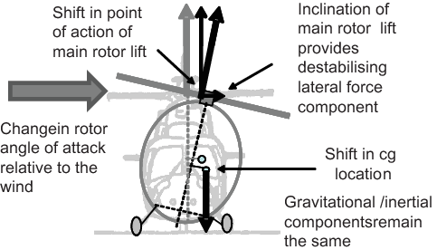
Figure 6. Destabilising effect of helicopter inclination relative to the helideck due to uneven oleo deflection.

It is possible to include all the above effects in the simple analytical ROS equations, if the relative deformation of the oleos/tyres can be calculated and/or the inclination of the helicopter relative to the helideck is known. However, quantifying this inclination presents some considerable difficulties since it can arise as follows:

• Due to the twist that can be generated in some undercarriage designs (e.g. Super Puma) as a result of landing with the brakes applied (helicopters land with one main wheel lower than the other as a result of the control forces needed to counteract the main rotor torque in the hover prior to landing).

• In response to the forces acting on the helicopter, making the oleo deformation and the forces implicitly related. The deflection response of the undercarriage is complex and non-linear, and such information is typically proprietary to helicopter OEMs.

• The undercarriage may respond dynamically to the transient forces acting on the helicopter; a simple quasi-static approach to modelling the forces acting on the helicopter could lead to an underestimate of any resonance effects or give an overestimation of forces by not accounting for inertial and/or damping effects. However, there does not seem to be any evidence to suggest that this could be a significant factor in practice.

As discussed later in 7.1.4, significant uneven undercarriage deflection seems to occur only as a result of oleo twist at landing, and this is now avoided in the UK since pilots are instructed to release and then re-apply the brake to allow the oleos to balance out after touchdown. Therefore, not including undercarriage deflection effects in the ROS modelling is not considered to be a significant omission and represents a very helpful simplification that avoids the additional modelling complexity and uncertainties discussed above.

6.0 CALCULATING THE ROS DIRECTLY FROM THE CONTACT REACTION FORCES

There is a direct, proportional relationship between the ROS and the helideck reaction forces.

In the case of tipping failure, the helideck reaction forces acting normal to the helideck balance the total weight of the helicopter (m·a_z). These reaction forces are distributed between the wheels in such a way as to exactly counterbalance the net restoring moment acting on the helicopter as a result of all the other external forces acting on the helicopter.

As part of this research programme, it has been shown that the ROS for tipping failure, for each of the tipping axes, can be expressed as a function of the normal reaction forces as follows:

(16)$$\matrix{ \matrix{ {\rm{RO}}{{\rm{S}}_{{\rm{TIP}}\_{\rm{NS}}}} = {{\rm{2}} \over {{{{\rm{CGX}}} \over {{\rm{FR}}}} - {{{\rm{CGY}}}\over{{\rm{LY}}}}}}\cdot{{{F_{{\rm{RP}}}}} \over {m\cdot{a_z}}} \hfill \cr {\rm{RO}}{{\rm{S}}_{{\rm{TIP}}\_{\rm{NP}}}} = {{\rm{2}} \over {{{{\rm{CGX}}} \over {{\rm{FR}}}} +{{{\rm{CGY}}} \over {{\rm{LY}}}}}}\cdot{{{F_{{\rm{RS}}}}} \over {m\cdot{a_z}}} \hfill \cr} \hfill \cr } $$

where F_RS, F_RP, are the normal reaction forces at the two main wheels (P and S), and CGY is assumed positive when offset towards starboard. Due to symmetry, the only difference in the expressions for NS and NP is in the sign of CGY. As expected, ROS_TIP=0 when either F_RS or F_RP are zero.

Thus, measuring the reaction forces provides a direct and exact way of calculating the ROS for tipping failure modes. It is possible to measure the helideck reaction forces normal to the helideck by placing the wheels of a helicopter on load cells. This method has been used successfully during helicopter trials offshore on the Foinaven FPSO and on the ground at Aberdeen airport.

The ROS for sliding failure can also, in principle, be measured in real time using load cells. This can be achieved by calculating the ratio of the total moment of the reaction forces acting on the wheels in the plane of the helideck (which, during equilibrium, is equal to the destabilising moment of the forces acting on the helicopter) divided by the maximum (restoring) frictional moment that can be generated by the vertical reaction forces, provided that the helideck coefficient of friction, μ, is known. This would be more complex to achieve in practice since it would require load cells capable of measuring the reaction forces in all three dimensions.

Finally, it is also possible to measure the reaction forces at the helicopter wheels by adding instrumentation directly to the helicopter undercarriage (e.g. using strain gauges). This is a promising idea, since it would allow the ROS (for tipping, and in principle also for sliding) to be measured in real time on an instrumented helicopter, providing an alarm to pilots if ROS_TIP and/or ROS_SLIDE were to drop to a dangerously low level. However, this is of limited use operationally, since pilots need to establish prior to landing whether on-deck conditions will be safe.

7.0 EXAMPLES OF IN-SERVICE ROS MODELLING AND VALIDATION AGAINST MEANSUREMENTS

The general analytical expressions for the ROS and the limits curves are precise, but the modelling of the individual forces acting on the helicopter is subject to a number of assumptions and uncertainties as discussed above. It was therefore necessary to evaluate the modelling against real-world measurements.

ROS values have been calculated and evaluated based on offshore on-deck datasets gathered from:

1. a) S-76 field trials onboard FPSO Foinaven (carried out in 1999).

2. b) the analysis of the G-BKZE Super Puma accident onboard the drill ship West Navion (in November 2001), carried out in collaboration with the UK Air Accidents Investigation Branch (AAIB).

A high-level summary of the main results and conclusions drawn from the analysis of this data is presented in the sections that follow.

7.1 S-76 Foinaven trials analysis

7.1.1 Introduction

The aim of the trials was to provide data to validate the helicopter stability model. DERA (the UK Defence and Evaluation Research Agency, now QinetiQ) had been subcontracted to carry out field trials onboard the FPSO Foinaven in November 1999, using an S-76 helicopter, operated by Bond Helicopters (now Babcock MCS).

Four tests were carried out, two with rotors stationary and two with rotors running at MPOG, both with the helicopter oriented aligned with the vessel’s longitudinal axis and at right angles to it (as illustrated in Fig. 7.)

Figure 7. S-76 trials onboard Foinaven: illustration of helicopter orientation and relative wind direction for each of the four tests.

Load cells were positioned under each of the wheels of the helicopter to measure the vertical reaction forces. The motion of the helideck was monitored using Motion Reference Units (MRUs), and the wind was measured with an ultrasonic anemometer located at the edge of the helideck.

The measured reaction forces were used to calculate the ROS directly using the method described in Section 6, and all other available information on deck motion and wind was used to reconstruct each of the forces and moments acting on the helicopter and to sum these to model the ROS.

7.1.2 Variations in vertical reactions due to deck motion

The first step in the evaluation of the results was to check that the variation in the sum of vertical reactions was as expected based on measurements of the deck motion. For the rotors stationary tests, this sum should be equivalent to the effective weight of the helicopter (= m^.a_z, assuming no lift forces are generated). The helicopter mass had been estimated (but was not exactly known) so this was adjusted to obtain a near-perfect agreement between the measured and modelled total vertical reactions trends, as shown in Fig. 8 below.

Figure 8. Rotors stationary tests: comparison of the sum of the vertical reactions (FZTexp) with the gravitational and inertial component normal to the deck (FGZmod).

7.1.3 Evaluating the main rotor lift model

Having obtained confidence in the calculation of the variation of the effective weight of the helicopter, the main rotor lift generated during rotors turning tests could then be calculated very accurately, by subtracting the effective weight from the measured sum of the vertical reaction forces. As shown in Fig. 9, the lift was equal to about 1,100 kgf or about 30% of the helicopter weight, with sizeable fluctuations of the order of +/-20% on either side of the mean.

Figure 9. The actual lift force (LIFTexp) was calculated from the difference between the sum of the measured vertical reactions (FZTexp) and the modelled gravitational and inertial component normal to the helideck (FGZmod).

Modelling the main rotor lift using the parametric lift equation (Equation 14) requires two main parameters, wind speed, U, and rotor disc angle of attack, α_s. Measurements of U (the wind speed in the plane of the helideck) during the trials are considered robust and were of the order of 10m/s (20 knots).

By contrast the accuracy of the values of α_s inferred from the trials measurements is uncertain. The anemometer readings indicated an updraft at the helideck that was very large (5m/s in a 12m/s wind (equivalent angle of 23°), far larger than the vertical wind component limit of ± 0.9m/s that used to form a limiting wind flow criterion in CAP437) now replaced with a limit on the standard deviation of the vertical airflow velocity. This could be the effect of localised flow distortion at the edge of the helideck, where the anemometer was mounted, which was not representative of the conditions at the centre of the helideck. Unfortunately, this has limited the extent to which the contribution of α_s in the parametric lift equation can be evaluated.

It is clear, however, that being able to match the measured main rotor lift with the equation is very sensitive to the choice of α_s. The value of α_s should also vary with the orientation of the helicopter rotor disk relative to the oncoming wind for any given incident wind updraft. As illustrated in Fig. 10, values for α_s were back-calculated to match the observed mean lift forces; as expected, these were different for different orientations to the wind, and were consistent with an updraft angle $ \uptheta_{\rm u} $ of about 4°.

Figure 10. Rotors turning tests: comparison of different ways of modelling the lift force, using a) a best fit constant value for the angle of attack as, b) no updraft, c) the mean wind speed recorded by the vessel and with zero updraft.

Regarding the prediction of the range of variation in the main rotor lift fluctuations either side of the mean, using the measured variation in U and a constant assumption for α_s reproduces some but not all of the observed variability; the peak values of lift in the actual lift time series are generally underpredicted.

7.1.4 The effect of oleo deformation

The inclinations of both the helideck and of the helicopter were measured. By subtracting the two, the helicopter inclination relative to the helideck was calculated. The mean relative inclination varied from test to test, from effectively zero in Test 4 to a maximum of 2° in Test 2, while variations relative to the mean were very small.

Any variability relative to the mean can only be attributed to deformations of the oleos/tyres in response to unequal wheel reactions (e.g. in roll, driven by RS - RP); these were found to be very small. However, the near constant differences in the mean inclination are more likely attributable to a constant uneven oleo deformation corresponding to twist in the undercarriage at touchdown. The differences observed during the trials were consistent with the negative, or left wing low roll attitude for an S-76 expected due to the direction of rotation of the main rotor and hence the direction of the tail rotor force.

Therefore, this is consistent with the quasi-static assumption in the analytical model that neglects effects due to the response of the undercarriage. A constant inclination correction to account for the possibility of undercarriage twist could easily be added to the measured helideck inclination.

7.1.5 Modelling lateral forces

The total lateral force/moment acting on the helicopter (using the location of the CoG as the reference) was inferred from the difference between the S and P wheel load cell measurements.

For rotors off tests, the agreement between the force inferred from the load cell measurements (exp) and a quasi-static calculation of the gravitational/inertial and fuselage drag forces (mod) was reasonable, as illustrated by the example shown in Fig. 11.

Figure 11. Test with rotors off — comparison of measured and modelled total side force.

By contrast, the total lateral force acting on the helicopter for rotors running tests was significantly higher than that during the rotors off tests (as illustrated in Fig. 12), suggesting that the main and/or tail rotors were generating net lateral moments.

Figure 12. Test with rotors on- comparison of measured and modelled total side force.

There are a number of possible explanations:

• Control forces were not equal to zero as assumed; FDR data of control settings during the trials were not obtained, so it is not known with certainty if the controls were indeed central during the trials.

• Even if cyclic and/or pedal controls were correctly centred, it is still possible that an additional drag force/moment could have been generated due to the interaction of the wind with the main rotor.

• A helicopter roll inclination relative to the helideck (e.g. due to uneven oleo deflection) could create a significant lateral component of main rotor lift, as well as increase the lateral gravitational component. Oleo deflection effects were not modelled in this example, but the helicopter was indeed inclined relative to the helideck during the tests by varying amounts in each test, and up to 2° on average.

The differences in the measured and modelled trends are plotted in Fig. 13. They act in a direction that adds to the destabilising effect of the wind, and their time variations seem to be correlated with main rotor lift force. This suggests that this additional side force is probably caused by the main rotor lift (rather than, for example, the tail rotor).

Figure 13. The difference in measured and modelled side force (FLATexp-FLATmod) for rotors turning tests.

Therefore, while it can be concluded that the modelling of lateral side forces in rotors stationary cases (i.e. due to deck motion and fuselage drag) is reasonably accurate, in the rotors turning tests additional sideways moments were generated that cannot currently be adequately accounted for with the approach presented in this paper, causing the overall modelled ROS to overpredict the actual ROS. Further work is recommended to improve this aspect of the modelling, based on an evidence-based understanding of the factors discussed previously in Section 5.4.

7.1.6 Modelling the ROS (tipping failure only)

The ROS for both tipping axes (NP and NS) was calculated in two ways:

1. a) ROS_TIPexp: directly from load cell measurements, using Equation (14).

2. b) ROS_TIPmod: the lift force was modelled using a constant value for α_s (giving the closest agreement with the measured lift, as previously discussed). The wind drag forces were calculated based on measured U, gravitational and inertial forces were calculated based on the MRU measurements of deck motion.

The results are compared in Fig. 14 below (only a subset of the time series modelled is shown for clarity).

Figure 14. Comparison of ROS calculated from measured reaction forces (exp) and that modelled (mod) using measured helideck accelerations and wind, and other helicopter-specific information.

When the rotors are stationary, the experimentally derived values R_TIPexp show that there is a modest reduction in the ROS. Comparing the modelled values to those derived experimentally for the rotors off tests, the agreement in Test 1 is very close, and the agreement in Test 4 is also good (the mean differs only by 5% and the max by 10%); this is consistent with the good agreement between the modelled and experimentally derived lateral forces.

When rotors are turning, there is a marked reduction in the experimentally derived ROS, down to a minimum of about 25%, compared to 75% when rotors were stationary. However, the modelled values underestimate this reduction by a significant margin (the worst-case minimum value is 42% instead of 25%). Since the lift was adjusted in this example to fit the experimental data, the difference between ROS_TIPexp and ROS_TIPmod reflects the effect of a significant rotor-induced lateral force which, as previously discussed, is not fully accounted for.

7.2 G-BKZE West Navion accident investigation

A tipping failure accident involving an AS332 L2 Super Puma (G-BKZE) occurred on the helideck of the West Navion drillship following a successful landing, disembarkation of passengers, and refuelling.

The helideck was within pitch, roll and heave limits. Owing to a failure in the ship’s dynamic positioning (DP) system, the heading of the vessel started drifting about 7 minutes after touchdown. After a further 5.5 minutes the aircraft tipped over, coming to rest on its side, causing significant damage to the aircraft, seriously injuring the co-pilot who was on the helideck outside the aircraft at the time, and damage to the surface of the helideck (Fig. 15).

Figure 15. Super Puma G-BKZE accident onboard the West Navion drillship, November 2001.

Several agencies had attempted to model the forces and moments acting on the helicopter when the accident occurred, and all were unable to explain why the helicopter had rolled over.

The Air Accidents Investigation Branch (AAIB) asked the authors to assist the investigation, using the numerical helicopter stability model that was being developed at the time. The model was used to establish whether helicopter tipping and/or sliding failure would have been expected given the available information from the accident.

The results from the stability model were consistent with the reported events and provided a clear and credible explanation of the accident. The calculation of the main rotor lift using Equation (14) was based on the mean wind speed quoted by the MetOffice, corrected for helideck height, and since the instantaneous wind speed/direction time series was not available, the lateral wind drag calculation was based on the mean reported wind speed and an inferred time variation in relative wind direction due to vessel heading control loss. The deck motion was based on the aircraft FDR data.

As shown in Fig. 16, the modelled tipping ROS trend dropped to zero at the time the tipping event actually occurred. The modelled ROS for sliding (for the N and S pivot modes) was also very close to zero prior to the tipping failure, and this is also consistent with the helicopter sliding momentarily prior to tipping over.

Figure 16. Modelled ROS_TIP (upper plot) and ROS_SLIDE for both sliding failure modes (lower plot), leading up to the time of the G-BKZE accident.

8.0 STRENGTHS AND LIMITATIONS OF THE MODELLING APPROACH

The modelling approach presented in this paper comprises three main components, each with its own strengths and limitations, as discussed below.

Analytical model for the Reserve of Stability (ROS): This is an exact, mathematical model derived from first principles, and applies generally to any unconstrained nose wheel tricycle helicopter on a moving helideck. It provides a transparent and clear framework for calculating the ROS and the relative contribution of deck motion and of all other destabilising factors, enabling the calculation of operational limits. Its main simplifying assumption is that the effect of deck motion and wind on helideck stability can be modelled quasi-statically, i.e. there is no dynamic response of the undercarriage and/or the rotor to deck motion. This appears to be an appropriate assumption for offshore operations, based on available data.

Simple parametric models of the forces acting on the helicopter (fuselage drag, main and tail rotor forces): These models were developed to calculate the external forces required as input by the analytical model, as a function of the most important (and minimum number of) helideck motion and wind parameters. Simplifications were chosen judiciously in order to capture as much of the main physics as possible while avoiding undue complexity. Comparisons against measurements, especially those made in-service, have been key to developing the models and evaluating their accuracy. As discussed in Section 7 above, this parametric modelling approach has been very useful in understanding the individual contributions to the ROS for the Foinaven trials, and for investigating the cause of the G-BKZE accident.

However, there are several areas where there are remaining uncertainties, and where improvements and further validation are recommended:

• The (mean) main rotor lift at MPOG has been modelled empirically as a function of wind speed and rotor disc angle of attack based on trials data for two helicopter types. It is not clear if this parameterisation applies more generally to other rotor types; even if only a tuning of its coefficients is required, this can only be done reliably based on helicopter type-specific trials. Instantaneous variations in lift due to wind fluctuations also need to be considered, since these can cause loss of stability in sufficiently high wind speeds — this is an aspect considered further in Part B, and further work is planned in this area.

• It is assumed that the main and tail rotors do not generate sideways forces/additional moments (other than those associated with the main rotor lift) when the control settings are centered, and that pilots will generally set the controls in a way that minimises any sideways forces. However, the analysis of the Foinaven trials data showed that additional destabilising moments were generated in the rotors turning cases, causing a significant reduction in ROS. As discussed previously in Section 5.4, there are several possible reasons and factors to consider which are not straightforward to quantify — the rigging of the helicopter rotor, the uncertainty in setting a neutral or central control setting, the interaction of the wind with the rotor, as well as the effect of deliberate or unintended control inputs by pilots.

• Effect of undercarriage deflection — the response of the helicopter undercarriage to the forces acting on the helicopter can be modelled in principle, and the associated displacements of the points of action and directions of each of the forces can be used in the analytical model to calculate the effect on the ROS. Furthermore, unintentional undercarriage deflections can occur at the time of landing due to an uneven compression of the oleos that cannot always be completely levelled out by releasing and re-applying the brake. Attempting to model undercarriage deflections would add considerable additional complexity (and a reliance on proprietary oleo data). Instead, the sensitivity of the ROS to a (given) range of undercarriage deflections could be quantified using the analytical model. Typical in-service undercarriage deflections can be deduced by comparing helicopter inclination data with the corresponding vessel motion data (e.g. for the Foinaven trials the maximum relative inclination was about 2°).

Quantifying inputs to represent operational scenarios: When modelling the ROS for any particular operational scenario, values need to be assigned to the inputs representing the operation-specific and ambient conditions (in addition to the helicopter type-specific coefficients needed for the parametric modelling discussed above). The accuracy of the ROS calculation is sensitive to inputs that can be difficult or impractical to capture, and which can vary significantly across operations, such as:

• operationally variable helicopter parameters (e.g. CGZ, mass, orientation at landing).

• differences between helidecks (e.g. susceptibility to updrafts/downdrafts, heading stability).

In addition, there will be variations in the helideck motion and the wind during each operation that will have to be quantified by reference to the MMS and MWS measured prior to landing:

• changes in the overall helideck motion and wind speed conditions after landing, compared to measurements taken prior to landing.

• instantaneous time variations (peaks) of helideck motion and wind speed during the on-deck duration.

Therefore, even with a perfect helicopter stability model, calculating the ROS for real offshore operational scenarios can only be meaningful if the inputs to the model are accurate and a representative range of variation is taken into account. This is discussed further in the second paper, Part B, where a probabilistic modelling approach to calculating limits is presented and discussed.

Additional measurements of the ROS gathered in-service in a variety of operational conditions (e.g. using an instrumented undercarriage), are also strongly recommended, to provide further insight into the accuracy and general applicability of the analytical modelling approach discussed above.