

Glacial isostatic adjustment (GIA) is a major mechanism responsible for crustal motion of the British Isles, mainly acting in a vertical direction. GIA is the visco-elastic reaction of the solid Earth to the glaciation and deglaciation of its surface. During the growth of a large continental ice sheet, the Earth's crust and mantle are displaced downwards and sideways, while the melting of an ice sheet and subsequent weight loss causes a reflux of the mantle and a mainly upward motion of the crust (postglacial rebound). This continues until a state of isostatic equilibrium is reached, which can be thousands of years after the deloading process. Aside from vertical land motion (VLM) of the Earth's crust, the redistribution of mass of surface ice, ocean water and mantle material also causes changes to the gravitational field of the Earth (Fleming et al. Reference Fleming, Johnston, Zwartz, Yokoyama, Lambeck and Chappell1998). Both aspects have a direct influence on relative sea-level (RSL) trends at the coast, which makes analysing and understanding the dynamics of GIA a critical task. The British GIA process, the effects of which are still prominent today, is mostly influenced by the disappearance of the Pleistocene British–Irish ice sheet and, to a lesser extent, by deglaciation effects of the Laurentide and Fennoscandian ice sheets (Hansen et al. Reference Hansen, Teferle, Bingley, Williams, Kenyon, Pacino and Marti2012). The last deglaciation of major global ice sheets began after the Last Glacial Maximum (∼22 kyr BP) (Shakun & Carlson Reference Shakun and Carlson2010) and lasted well into the early Holocene (∼7 kyr BP) (Milne et al. Reference Milne, Shennan, Youngs, Waugh, Teferle, Bingley, Bassett, Cuthbert-Brown and Bradley2006). Crustal uplift and relative land-/sea-level changes in the British Isles occur with considerable spatial and temporal variability, reflecting the influences of the different former ice sheets. Both the postglacial rebound of the crust and the eustatic sea-level changes associated with meltwater influx were comparable in magnitude (Shennan et al. Reference Shennan, Peltier, Drummond and Horton2002). When analysing vertical land motions, several other factors should also be taken into account. These include smaller local tectonic movements, far-field effects of, for example, Alpine crustal motion and flexural effects, including shelf loading associated with eustatic sea-level fluctuations. Further processes are continental erosion, subsidence due to sediment compaction or water, gas and oil pumping, and deep mining operations, which took place until the 1980s in the UK (Soudarin et al. Reference Soudarin, Crétaux and Cazenave1999; Teferle et al. Reference Teferle, Bingley, Orliac, Williams, Woodworth, McLaughlin, Baker, Shennan, Milne and Bradley2009). In terms of sea-level changes, there are also local effects, such as tide regime changes and/or sedimentation processes along the coast (Shennan et al. Reference Shennan, Milne and Bradley2009).
Many different methods for inferring vertical land motions and/or relative land- and sea-level changes, incorporating different observational data types, have been employed to obtain information for constraining model parameters in GIA modelling. These methods encompass the analysis of GIA through geological reconstructions of Late Pleistocene and Holocene relative sea-level changes (e.g., Peltier & Andrews Reference Peltier and Andrews1976; Clark et al. Reference Clark, Farrell and Peltier1978; Tushingham & Peltier Reference Tushingham and Peltier1991); and through modern geodetic techniques, such as determining changes in the gravity field (e.g., Mitrovica & Peltier Reference Mitrovica and Peltier1989), or three-dimensional crustal motions measured by very long baseline interferometry (VLBI) and GPS (e.g., James & Lambert Reference James and Lambert1993; Mitrovica et al. Reference Mitrovica, Davis and Shapiro1993; Milne et al. Reference Milne, Davis, Mitrovica, Scherneck, Johansson, Vermeer and Koivula2001; MacMillan & Boy Reference MacMillan, Boy, Vandenberg and Baver2004). Both types of field observations – geological and geodetic – have been used to inform GIA models. However, there is a significant difference in the observational time scale between these two data sets. The geological information describes the long-term development of GIA/RSL since the Last Glacial Maximum (LGM). Modern geodetic observations, on the other hand, give direct and accurate measurements of short-term or present-day GIA for the past few decades only. Geodetic data can help constrain GIA models, but the long-term nature of the postglacial rebound process means that modelling relies heavily on Late Devensian and Holocene long-term data for calibration and parameterisation of ice history and mantle rheology. The short-term geodetic time-series data generally cannot fully explain those long-term trends, or any periodic signals in the vertical land motion. For instance, the current VLM estimates (for the past 1–2 decades) and the long-term geologically derived VLM rates differ by 0.7 to −1.3 mm yr–1, with the uplift in Scotland and the subsidence in southwest England being lower in the geodetic short-term results (BIGF 2014).
This paper is an introductory overview of the different existing analytical methods of observing relative sea-/land-level change and GIA-induced vertical land motion and it summarises different modelling approaches to glacial isostatic adjustment for the British Isles. The suitability of relatively new methods for measuring VLM, such as SAR interferometry (InSAR), is also explored. The approach in this paper is mainly chronological, but distinguishes the two principal methodologies of using (i) long-term Late Devensian/Holocene geological (sea-level) data and (ii) present-day geodetic measurements for GIA quantification (in sections 2 and 3, respectively).
In this paper, Section 1 introduces necessary terminology and reference systems for the discussion of different research techniques. Section 2 focuses on using past relative sea-level changes to analyse GIA, with section 2.1 giving a short introduction to the publications responsible for an extensive high-quality sea-level change data set derived from geological information from various palaeo-environments between the LGM and the present (e.g., Sissons Reference Sissons1962, Reference Sissons1963, Reference Sissons1966, Reference Sissons1972, Reference Sissons, Smith and Dawson1983; Sissons et al. Reference Sissons1966; Smith et al. Reference Smith, Morrison, Jones, Cullingford, Cullingford, Davidson and Lewin1980, Reference Smith, Firth, Turbayne and Brooks1992, Reference Smith, Firth, Brooks, Robinson and Collins1999, Reference Smith, Cullingford and Firth2000, Reference Smith, Firth and Cullingford2002, Reference Smith, Haggart, Cullingford, Tipping, Wells, Mighall and Dawson2003a, Reference Smith, Fretwell, Cullingford and Firth2006, Reference Smith, Cullingford, Mighall, Jordan and Fretwell2007, Reference Smith, Davies, Brooks, Mighall, Dawson, Rea, Jordan and Holloway2010, Reference Smith, Hunt, Firth, Jordan, Fretwell, Harman, Murdy, Orford and Burnside2012; Shennan et al. Reference Shennan, Tooley, Davis and Haggart1983, Reference Shennan, Innes, Long and Zong1993, Reference Shennan, Smith and Dawson1994, Reference Shennan, Innes, Long and Zong1995a, Reference Shennan, Innes, Long and Zongb, Reference Shennan, Hamilton, Hillier and Woodroffe2005, Reference Shennan, Hamilton, Hillier, Hunter, Woodall, Bradley, Milne, Brooks and Bassett2006b; Firth Reference Firth1984; Shennan Reference Shennan and Devoy1987, Reference Shennan1999; Cullingford et al. Reference Cullingford, Smith and Firth1991; Firth et al. Reference Firth, Smith, Hansom and Pearson1995; Shennan & Horton Reference Shennan, Peltier, Drummond and Horton2002). Section 2.2 discusses specifically the development and refinement of empirical and theory-driven GIA models and the constraining of their parameters, using these geological data (e.g., Lambeck Reference Lambeck1993a, Reference Lambeckb, Reference Lambeck1995; Lambeck et al. Reference Lambeck, Johnston, Smither and Nakada1996; Peltier Reference Peltier1998a; Shennan et al. Reference Shennan, Lambeck, Horton, Innes, Lloyd, McArthur, Purcell and Rutherford2000, Reference Shennan, Peltier, Drummond and Horton2002, Reference Shennan, Bradley, Milne, Brooks, Bassett and Hamilton2006a). Section 2.3 compares published maps of relative sea- and land-level changes based on the application of geological information (e.g., Shennan & Horton Reference Shennan, Peltier, Drummond and Horton2002; Smith et al. Reference Smith, Fretwell, Cullingford and Firth2006, Reference Smith, Hunt, Firth, Jordan, Fretwell, Harman, Murdy, Orford and Burnside2012; Shennan et al. Reference Shennan, Milne and Bradley2009, Reference Shennan, Milne and Bradley2012).
Section 3 gives an insight into the literature that focuses on using geodetic techniques to analyse British Isles GIA. Such geodetic studies have used continuous GPS (CGPS) and absolute gravity (AG) measurements to determine crustal motions of the British Isles (section 3.1) (e.g., Teferle et al. Reference Teferle, Bingley, Dodson and Baker2002, Reference Teferle, Bingley, Williams, Baker and Dodson2006, Reference Teferle, Williams, Kierulf, Bingley and Plag2008, Reference Teferle, Bingley, Orliac, Williams, Woodworth, McLaughlin, Baker, Shennan, Milne and Bradley2009), and those measurements have been used to improve the parameterisation of GIA models (section 3.2) (e.g., Milne et al. Reference Milne, Shennan, Youngs, Waugh, Teferle, Bingley, Bassett, Cuthbert-Brown and Bradley2006; Bradley et al. Reference Bradley, Milne, Teferle, Bingley and Orliac2009, Reference Bradley, Milne, Shennan and Edwards2011). Section 3.3 discusses the possibilities of using InSAR for measuring crustal motion in mainland Scotland, where the signal of vertical land uplift is predominant.
1. Definition of terms and reference systems
The fact that the measuring and modelling techniques explored in this paper rely on various vertical reference systems has to be kept in mind when comparing the vertical land motion or relative sea-level change output of these different methods (see Figure 1 for schematic representation). The following represents a description of these reference systems, as well as a summary of the most commonly used terminology. Most cited literature in this paper can be understood against this background, although it is important to note that different meanings have emerged over the years for specific technical terms. Thus, when comparing methods and results between papers, caution is required; especially if these papers have been written with a different perspective – from a geological, geodetic or GIA modelling field of research. Shennan et al. (Reference Shennan, Milne and Bradley2012) discuss the ambiguity of terminology in sea-level research in more detail.
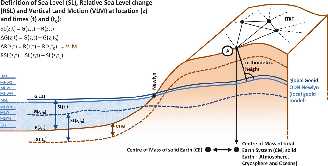
Figure 1 Schematic overview of reference surfaces used when measuring and modelling RSL change and vertical land motion (VLM) of the British Isles (after Shennan et al. Reference Shennan, Milne and Bradley2012, extended). Sea level (SL) at time t and location z is defined as the distance between Geoid (G) and solid Earth surface (R), which both relate to the centre of the Earth. G is the long-term averaged mean sea surface over several decades (Shennan et al. Reference Shennan, Milne and Bradley2012). Around Great Britain, the global Geoid lies about 80 cm above a local geoid model (Ordnance Datum Newlyn – ODN) due to sea surface topography. ODN is defined by mean sea level measured at Newlyn tide gauge between 1915 and 1921. Orthometric height of a point A is height above ODN (Ordnance Survey 2015). Eustatic sea-level change and isostatic changes to the gravitational field can cause change in G between a time t and a reference time t0. VLM is the change in solid Earth surface R between a time t and t0. RSL change refers to the difference in sea level (SL) at a time t relative to t0. Variations in water levels from MSL are indicated on the left hand side for a semidiurnal tidal system (for definitions see main text and Woodroffe & Barlow Reference Woodroffe, Barlow, Shennan, Long and Horton2015; Shennan Reference Shennan, Shennan, Long and Horton2015). MHWS and HAT are a common reference of sea-level index points or isobase models of RSL change. ITRF is the International Terrestrial Reference Frame mostly used for GPS referencing (ITRF2008 is the latest one), relative to the CM of the total Earth System. CE is used in GIA modelling.
With regard to the reconstruction of past relative sea-level change, height measurements of sea-level index points are initially taken relative to Ordnance Datum Newlyn (ODN); for example, by levelling to local benchmarks (Sissons Reference Sissons1962, Reference Sissons1963; Sissons et al. Reference Sissons1966; Shennan Reference Shennan1982). ODN is defined after local mean sea level (MSL) that was observed between 1915 and 1921 at the tide gauge in Newlyn, Cornwall and is closely approximated by a local geoid model that deviates from the global Geoid by about 80 cm. Heights above MSL in Great Britain usually relate to this vertical datum (Ordnance Survey 2015).
MSL is more generally defined as the arithmetic mean of hourly elevation measurements at a certain location for a specific period (≥19 years) (Woodroffe & Barlow Reference Woodroffe, Barlow, Shennan, Long and Horton2015). After the geodetic definition, MSL is not a level surface and it does not exactly follow the Geoid, which is an equipotential surface. This is due to ocean dynamic effects, such as tidal forcing, ocean currents, atmospheric processes and changes in ocean density, which cause sea surface topography. MSL and the Geoid lie close together, but can deviate from each other by a few decimetres, even after averaging for tidal effects (Woodroffe & Barlow Reference Woodroffe, Barlow, Shennan, Long and Horton2015).
It should be noted here that Shennan et al. (Reference Shennan, Milne and Bradley2012) emphasise the differentiation between the terms ‘relative land- and sea-level change’ and ‘vertical land motion’. Trying to find a common terminological ground for the GIA community, they describe sea level as the distance between the Geoid (G) (see Fig. 1), which is defined as the global time-averaged sea surface over several decades, and the solid Earth surface (R) (see also Mitrovica & Milne Reference Mitrovica and Milne2003). ‘Relative’ change always involves not only a change in elevation between the Geoid and the solid Earth surface, but also a change between a point in the past relative to the present day. R and G are relative to the centre of the Earth. Relative sea-level change is the negative of relative land-level change. Vertical land motion, in contrast, refers only to the change in elevation of the solid surface of the Earth relative to its centre. The difference between VLM and relative land-level change accounts for approximately −0.1 to −0.3 mm yr–1 around the British Isles and +2.5 to −1.5 mm yr–1 globally (Shennan et al. Reference Shennan, Milne and Bradley2012; Shennan Reference Shennan, Shennan, Long and Horton2015). Vertical land motion, combined with eustatic sea-level change, results in the relative land-/sea-level change rate. If both eustatic sea level and VLM changed at the same rate in the same direction, no RSL change would be detectable.
The term ‘eustatic’ generally corresponds to changes in the volume of water in the ocean (Farrell & Clark Reference Farrell and Clark1976) and is used in the GIA modelling community to describe the glacio-eustatic component caused by volume changes of land surface-based ice. Any other contributions to eustasy (Fairbridge Reference Fairbridge1961) are neglected, such as a change in ocean basin geometry (tectono-eustasy) and changes in density due to variability in the heat and salinity budget of the oceans (steric effects) (Fleming et al. Reference Fleming, Johnston, Zwartz, Yokoyama, Lambeck and Chappell1998; Peltier Reference Peltier2002; Milne & Mitrovica Reference Milne and Mitrovica2008; Bradley et al. Reference Bradley, Milne, Shennan and Edwards2011).
In addition, sea-level index points usually refer to different reference water or tide levels; thus, a standardisation of the points to present mean tide level (MTL) is necessary when deriving the RSL change values (Shennan et al. Reference Shennan, Innes, Long and Zong1995a). MTL is the average of mean high and mean low water (MHW/MLW) at a location. Other levels for a semidiurnal tidal system include HAT (highest astronomical tide), MHWS (mean high water springs), MHW (mean high water), MHWN (mean high water neaps), MLWN (mean low water neaps), MLW (mean low water), MLWS (mean low water springs), LAT (lowest astronomical tide) and CD (chart datum); (for a description see Woodroffe & Barlow Reference Woodroffe, Barlow, Shennan, Long and Horton2015). Isobase models of relative sea-level (RSL) change rely on height measurements relative to ODN and are then adjusted to heights above MHWS, the average spring tide high water level measured over a certain period (Smith et al. Reference Smith, Hunt, Firth, Jordan, Fretwell, Harman, Murdy, Orford and Burnside2012; Woodroffe & Barlow Reference Woodroffe, Barlow, Shennan, Long and Horton2015). Continuous GPS measurements of VLM are mostly relative to a global network of points with known coordinates, the International Terrestrial Reference Frame (ITRF) or regional subsets thereof, which in turn depend on its origin at the long-term mean of the centre of mass of the total Earth system (CM) (Altamimi et al. Reference Altamimi, Collilieux and Métivier2011). Absolute gravimetry (AG) also takes gravity – and, subsequently, height – measurements relative to the Earth system's centre of mass. GIA models often use the centre of mass of the solid Earth (CE) as a reference, which deviates slightly from the CM (Collilieux & Altamimi Reference Collilieux, Altamimi and Sideris2013).
Furthermore, the term ‘vertical land motion’ represents a combination of all vertical deformation effects in an area, not only GIA-induced vertical crustal motion. Strictly speaking, direct geodetic measurement techniques, such as continuous GPS or InSAR, can only be used to acquire information about the net vertical glacial rebound process when all other vertical deformation effects can be neglected. However, the crustal uplift caused by GIA can be seen as the dominant process of VLM of the British Isles over a long-term period, so that the geodetic methods can be used as a good indicator of GIA (Bradley et al. Reference Bradley, Milne, Teferle, Bingley and Orliac2009; Hansen et al. Reference Hansen, Teferle, Bingley, Williams, Kenyon, Pacino and Marti2012).
2. Geological evidence and GIA modelling
Geological sea-level research is based on the fact that a change of sea level influences stratigraphical successions at the coast. Deposits provide information about freshwater, marine or terrestrial sedimentation processes. Relative sea-level changes during the Holocene can be reconstructed using observations derived from chronological, morphological, stratigraphical and palaeontological analyses at transition zones between marine and terrestrial sediments in different locations along the coast. These analyses are undertaken on, ideally unconsolidated, organic and minerogenic sediments and morphological features that are related to palaeo sea levels and have been undisturbed by erosion or transportation since their formation (Shennan et al. Reference Shennan, Innes, Long and Zong1995a, Reference Shennan, Bradley, Milne, Brooks, Bassett and Hamilton2006a). Records can stem from basal or freshwater peats, partly intercalated between layers of clastic sediments, and intertidal sediment deposits of silts, clays and sands from estuaries and coastal lowlands. These are found, for instance, in subsidence areas of England, but also on the east coast of Scotland (Shennan Reference Shennan1992; Shennan et al. Reference Shennan, Innes, Long and Zong1994). In uplift areas, emerged coastal features such as raised rock platforms and beaches, gravel ridges (Reference Altamimi, Collilieux, Legrand, Garayt and BoucherFig. 2) or isolation basins (Reference Altamimi, Collilieux and MétivierFig. 3) play an important role. Tidal marshes, coastal wetlands and dune systems have also been analysed (Shennan et al. Reference Shennan, Hamilton, Hillier and Woodroffe2005).
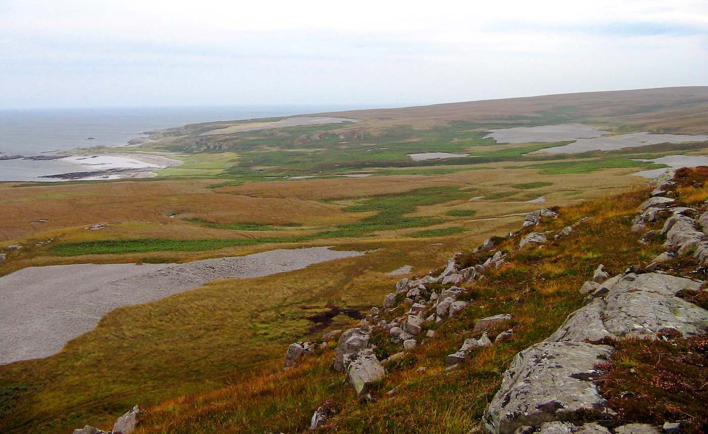
Figure 2 Staircases of emerged gravel ridges uplifted by glacial isostatic adjustment at Shian Bay, Isle of Jura. The highest ridge is about 35m ASL (see Castillo et al. Reference Castillo, Bishop and Jansen2013). In the right foreground is a glacially striated roche moutonnée.

Figure 3 Isolation basin in northwestern Scotland, separated from the influences of the sea and its highest tides.
A problem is that sediments are often spatially and temporally discontinuous, due to disruption by land surface processes and climate change, so that a comparison of different sites becomes difficult. A common classification method in RSL reconstruction defines sea-level index points. Important groundwork for establishing sea-level curves from sea-level index points has been laid by Tooley (Reference Tooley1974b, Reference Tooley1978, Reference Tooley1982a, Reference Tooleyb) and van de Plassche (Reference Van de Plassche1982), followed by a methodological approach from Shennan (Reference Shennan, Smith and Dawson1984, Reference Shennan1986a, Reference Shennanb; Shennan et al. Reference Shennan, Tooley, Davis and Haggart1983, Reference Shennan, Innes, Long and Zong1995a) that allows the correlation of sea-level index points in different geological and geomorphological palaeo-environments on spatial and temporal scales. This happens by defining a set of characteristics, namely age, location and altitude, indicative meaning and tendency of sea-level movement. Age is determined by radiocarbon (14C) dating the organic samples, supported by microfossil (pollen and diatom) analyses (Shennan Reference Shennan1982). Altitude is initially measured above ODN by levelling. Time and altitude are generally not enough to give unambiguous clues about sea-level falls and rises, which is why other characteristics have to be determined in order to establish relative sea-level movements. A chronology of sea-level tendencies gives information about direction of movement of sea level (Tooley Reference Tooley1978; van de Plassche Reference Van de Plassche1982; Shennan Reference Shennan1982, Reference Shennan, Smith and Dawson1984; Shennan et al. Reference Shennan, Tooley, Davis and Haggart1983). This allows separation of transgression and regression overlaps in the sediments, indicated by vegetation and/or lithology changes. This includes the alternation of terrestrial or freshwater sediments with marine sediments due to eustatic sea-level changes, land uplift or subsidence and changes in sedimentation rate and deposited material (Tooley Reference Tooley1982b). The indicative meaning places a sample's location in relation to a contemporary reference tide level, so that comparisons between various sampling areas are possible. Depending on the type of deposited material, this can refer to mean high water of spring tides (MHWS), mean tide level (MTL) or highest astronomical tide (HAT) (Shennan Reference Shennan1992; Shennan et al. Reference Shennan, Innes, Long and Zong1995b) (see also Reference AdamskaFig. 1). Additionally, an indicative range gives information about the accuracy of the indicative meaning. Finally, in order to determine rates of RSL change, a linear trend is aligned to the age–sea-level height plots of observations (Shennan Reference Shennan1989; Shennan & Horton Reference Shennan and Horton2002).
2.1. Building up a data bank of Late Devensian and Holocene sea-level observations
Since the late 20th Century, several studies have been undertaken to collect data on Late Devensian and Holocene relative sea-level change from palaeo-environments in Great Britain; thus accumulating a rich data bank of sea-level index points that help constrain GIA model parameters and reduce existing model discrepancies (e.g., Tooley Reference Tooley1974b; Shennan Reference Shennan1989; Shennan et al. Reference Shennan, Innes, Long and Zong1995a, Reference Shennan, Lambeck, Horton, Innes, Lloyd, McArthur, Purcell and Rutherford2000, Reference Shennan, Hamilton, Hillier and Woodroffe2005, Reference Shennan, Bradley, Milne, Brooks, Bassett and Hamilton2006b; Shennan & Horton Reference Shennan and Horton2002). Extending the comprehensive analysis by Shennan (Reference Shennan1989) of all then-available radiocarbon data on sea-level index points, Shennan et al. (Reference Shennan, Innes, Long and Zong1995a) summarised the information gained from various studies undertaken in northwestern Scotland (between Kentra Bay and Loch Morar) (Shennan et al. Reference Shennan, Innes, Long and Zong1993, Reference Shennan, Innes, Long and Zong1994, Reference Shennan, Innes, Long and Zong1995b). Previous studies had focused predominantly on eastern, northeastern and southern Scotland (Sissons et al. Reference Sissons1966), or the east coast of England (Shennan Reference Shennan1992), where sedimentary environments for sea-level research are available in abundance. Few stratigraphic studies had been undertaken in western Scotland prior to Shennan et al.'s studies, due to the lack of appropriate depositional or sedimentary environments in that region, except for the southwestern part of Scotland (e.g., Jardine Reference Jardine1980).
The rest of Great Britain, in contrast, exhibits more wide-ranging estuarine deposits that can be used for GIA studies. Shennan et al. (Reference Shennan, Innes, Long and Zong1995a) thereby established a broad data set of Late Devensian and Holocene relative sea-level changes from 12 kyr 14C BP to the present, the main elements of which are a rapid fall of sea level of about 9 mm/14C yr before 10 kyr 14C BP, followed by an almost stationary sea level in the early Holocene, which was succeeded by a rise of sea level to a mid-Holocene highstand, with a subsequent fall in the Late Holocene (Shennan et al. Reference Shennan, Lambeck, Horton, Innes, Lloyd, McArthur, Purcell and Rutherford2000).
Shennan et al. (Reference Shennan, Hamilton, Hillier and Woodroffe2005) added new sea-level index point observations to that database from isolation basins, raised tidal marshes, coastal wetlands and dune systems located around Arisaig, northwest Scotland. They created a 16,000-year record of relative sea-level changes from the time of deglaciation after the Last Glacial Maximum to the present. In particular, they presented new data on the mid-Holocene RSL highstand (reached between ∼7,600–7,400 cal yr BP and 6.74±0.2 m above present) and on the Laurentide and Antarctic ice sheet duration.
Other studies within a second school of thought of RSL research have also contributed substantially to the observational information about Holocene RSL change. These focused on collecting direct altitude measurements along prominent palaeo-shorelines in sheltered inlets and estuaries, and provided chronological information from stratigraphical analyses, instead of chronological and altitudinal analyses in isolation basins. The shoreline data have been used to model isobase maps of the pattern of uplift in Scotland (see also section 2.3).
Raised shorelines, caused by glacio-isostatic uplift, are basically marine limits at inland margins that are characterised by distinctive features in their morphology and stratigraphy (Smith et al. Reference Smith, Cullingford and Firth2000). The temporal sequence of raised shorelines during the Holocene enables the reconstruction of Holocene uplift patterns. Early investigations on visible and buried raised beaches, with shoreline altitudinal measurements and detailed morphological analyses in Scotland were conducted by Sissons (Reference Sissons1962, Reference Sissons1963, Reference Sissons1966, Reference Sissons1969), Sissons et al. (Reference Sissons1966), Smith (Reference Smith1968), Smith et al. (Reference Smith, Thompson and Kemp1978), Kemp (Reference Kemp1976), Dawson (Reference Dawson1979, Reference Dawson1980, Reference Dawson1984) and Firth & Haggart (Reference Firth and Haggart1989). The work of Sissons and co-workers (e.g., Sissons Reference Sissons1962, Reference Sissons1963; Sissons et al. Reference Sissons1966) provided an important re-definition of raised shorelines and their heights, with a focus on southeast Scotland, by pioneering the application of levelling techniques based on OD benchmarks.
Among the four main and most visible shorelines is the Storegga Slide Tsunami Shoreline, which has been analysed, for example, by Smith et al. (Reference Smith, Cullingford and Firth2000, Reference Smith, Shi, Cullingford, Dawson, Dawson, Firth, Foster, Fretwell, Haggart and Holloway2004, Reference Smith, Fretwell, Cullingford and Firth2006, Reference Smith, Hunt, Firth, Jordan, Fretwell, Harman, Murdy, Orford and Burnside2012) and Dawson et al. (Reference Dawson, Bondevik and Teller2011). The shoreline reached immediately before the tsunami struck along the east coast of Scotland in the mid Holocene, is dated at around 8,100 cal yr BP (Dawson et al. Reference Dawson, Bondevik and Teller2011). Smith et al. (Reference Smith, Cullingford and Firth2000) used altitude observations, along with stratigraphic and microfossil analysis of sediments at the inner margin of the estuarine surface at the time of the tsunami, thus enabling the modelling of uplift of mainland Scotland since the tsunami. Deposition of tsunami sediments was rapid and essentially synchronous at each coastal location, thereby avoiding diachroneity that often compromises the determination of the uplift pattern in glacial rebound areas (Smith et al. Reference Smith, Shi, Cullingford, Dawson, Dawson, Firth, Foster, Fretwell, Haggart and Holloway2004).
Altitudinal data have also been collected from the Main Postglacial Shoreline and analysed by Sissons et al. (Reference Sissons1966), Smith (Reference Smith1968), Sissons (Reference Sissons1972, Reference Sissons, Smith and Dawson1983), Smith et al. (Reference Smith, Morrison, Jones, Cullingford, Cullingford, Davidson and Lewin1980, Reference Smith, Firth, Turbayne and Brooks1992, Reference Smith, Firth, Brooks, Robinson and Collins1999, Reference Smith, Cullingford and Firth2000, Reference Smith, Firth and Cullingford2002, Reference Smith, Haggart, Cullingford, Tipping, Wells, Mighall and Dawson2003a, Reference Smith, Wells, Mighall, Cullingford, Holloway, Dawson and Brooksb, Reference Smith, Fretwell, Cullingford and Firth2006, Reference Smith, Cullingford, Mighall, Jordan and Fretwell2007, Reference Smith, Davies, Brooks, Mighall, Dawson, Rea, Jordan and Holloway2010, Reference Smith, Hunt, Firth, Jordan, Fretwell, Harman, Murdy, Orford and Burnside2012), Dawson (Reference Dawson1984), Firth (Reference Firth1984), Cullingford et al. (Reference Cullingford, Smith and Firth1991), Firth et al. (Reference Firth, Smith, Hansom and Pearson1995), Selby & Smith (Reference Selby and Smith2007) and Jordan et al. (Reference Jordan, Smith, Dawson and Dawson2010), among others. This shoreline is dated at 6,400–7,700 cal yr BP, when the Main Postglacial Transgression occurred (Mcintyre & Howe Reference Mcintyre and Howe2010). It was for a long time believed to be the highest shoreline, but the Blairdrummond Shoreline, modelled by Smith et al. (Reference Smith, Cullingford and Firth2000, Reference Smith, Fretwell, Cullingford and Firth2006, Reference Smith, Cullingford, Mighall, Jordan and Fretwell2007, Reference Smith, Hunt, Firth, Jordan, Fretwell, Harman, Murdy, Orford and Burnside2012), overlaps with the Main Postglacial Shoreline at the margin of glacio-isostatic uplift (Smith et al. Reference Smith, Cullingford, Mighall, Jordan and Fretwell2007, Reference Smith, Hunt, Firth, Jordan, Fretwell, Harman, Murdy, Orford and Burnside2012). The Blairdrummond Shoreline has been dated at 4,500–5,800 cal yr BP (Mcintyre & Howe Reference Mcintyre and Howe2010). Smith et al. (Reference Smith, Fretwell, Cullingford and Firth2006, Reference Smith, Hunt, Firth, Jordan, Fretwell, Harman, Murdy, Orford and Burnside2012) also mention the Wigtown Shoreline, which is visible in a terrace below the Blairdrummond Shoreline and dated at 1,520–3,700 cal yr BP (Mcintyre & Howe Reference Mcintyre and Howe2010). A note on the empirical modelling approaches based on this shoreline data, compared to the more theory-driven, rheological GIA models, is given in the following section.
2.2. GIA modelling approaches constrained by Late Devensian and Holocene RSL data
These kinds of high-quality and long-term sea-level reconstructions around the British Isles have been used for model calibration and validation in a range of studies developing high-resolution glacio-isostatic rebound models of the British Isles (e.g., Lambeck Reference Lambeck1993a, Reference Lambeckb, Reference Lambeck1995; Lambeck et al. Reference Lambeck, Johnston, Smither and Nakada1996; Shennan et al. Reference Shennan, Lambeck, Horton, Innes, Lloyd, McArthur, Purcell and Rutherford2000, Reference Shennan, Peltier, Drummond and Horton2002, Reference Shennan, Bradley, Milne, Brooks, Bassett and Hamilton2006a; Peltier et al. Reference Peltier2002; Milne et al. Reference Milne, Shennan, Youngs, Waugh, Teferle, Bingley, Bassett, Cuthbert-Brown and Bradley2006).
GIA models usually encompass (1) an Earth-model for the isostatic signal that is related to the solid Earth deformation due to surface mass redistribution between ice sheets and oceans; (2) a model of the ice sheet evolution during the Late Pleistocene; and (3) a (sea-level change) model for the re-distribution of ocean water resulting from ice mass changes, incorporating the sea-level equation (Milne et al. Reference Milne, Shennan, Youngs, Waugh, Teferle, Bingley, Bassett, Cuthbert-Brown and Bradley2006; Shennan et al. Reference Shennan, Bradley, Milne, Brooks, Bassett and Hamilton2006a). Earth-models in GIA modelling usually contain several layers of varying densities, elastic parameters and viscosities, for which various values can be found in the literature (see Reference Aobpaet, Cuenca, Hooper and TrisirisatayawongFig. 4). These layers include a lithosphere with a certain thickness, one or more upper-mantle layers with different viscosities – alternatively a more detailed depth-dependent viscosity structure – and a lower mantle viscosity below the 670 km seismic discontinuity. The Earth-model is usually described by a spherically symmetric, self-gravitating Maxwell body (Bradley et al. Reference Bradley, Milne, Shennan and Edwards2011).

Figure 4 Earth-model configurations in GIA studies mentioned in this paper.
For the ice-model, parameters such as ice sheet dimensions and thickness and the temporal evolution of ice build-up and melting are significant over the entire Late Pleistocene/Holocene period, since the effects of (melt-)water loading and the ice-equivalent eustatic contribution on the RSL observations (including any major meltwater pulses) have a major influence on model output.
The UK sea-level dataset provides important constraints on GIA model parameters, such as lithospheric thickness, upper mantle viscosity, near-field ice sheet history of the British Isles, global/far-field deglaciation history and magnitude and rate of global meltwater discharge (Shennan et al. Reference Shennan, Hamilton, Hillier and Woodroffe2005). However, the modelling studies also show that observations are difficult to fit with a single ice-Earth-model combination, and no unique solution has been found for the explanation of relative sea-level observations; one reason being the sensitivity of the GIA process to both near- and far-field effects (Milne et al. Reference Milne, Shennan, Youngs, Waugh, Teferle, Bingley, Bassett, Cuthbert-Brown and Bradley2006). Great Britain's proximity to Fenno-Scandinavia and the large mass of the former Fennoscandian ice sheet mean that RSL and glacial rebound are not only influenced by the former British–Irish ice sheet. Additional contributions by loading–unloading of the crust due to the Fennoscandian ice sheet, its meltwater and gravitational attraction of the ocean water, have to be taken into account in Scottish GIA modelling (Lambeck Reference Lambeck1991). Present-day uplift in Fennoscandia can reach up to 10 mm yr–1, calculated, for example, from long-term tide gauge records and corrected with a eustatic sea-level rise of 1.2 mm yr–1 (Steffen & Wu Reference Steffen and Wu2011). Absolute gravity and continuous GPS measurements show the same rate, with an uplift centre in the northern Gulf of Bothania (Johansson et al. Reference Johansson, Davis, Scherneck, Milne, Vermeer, Mitrovica, Bennett, Jonsson, Elgered, Elosegui, Koivula, Poutanen, Ronnang and Shapiro2002; Steffen & Wu Reference Steffen and Wu2011).
Lambeck (Reference Lambeck1993a, Reference Lambeckb) provided the first comprehensive modelling studies of British sea-level evidence and discussed parameterisation of the Earth-model and ice-model that determines the sea-level predictions. Both papers developed a forward-modelling-inverse-modelling process that allows determination of the optimum ice sheet (ice thickness and ice sheet margins) and Earth rheology parameters for Great Britain for the Late Pleistocene and Holocene from the then-existing geological sea-level data. Lambeck (Reference Lambeck1993a) formulated the requirements for simulating the glacial rebound with a high precision and resolution of better than 1m, such as inclusion of the Fennoscandian ice sheet for far-field effects, consideration of different ice sheet load cycles and the Loch Lomond Readvance. Including sea-level observations from inside and outside of the glacial margins allowed separation of Earth-model parameters from ice sheet parameters in the inversion of the GIA equations. Starting with a simple first- and second-order rebound model in Lambeck (Reference Lambeck1993a), the author eventually presents a more complex GIA model (Lambeck Reference Lambeck1993b). This includes a more detailed ice-model for the Late Devensian ice sheet for the period between maximum glaciation and the end of the Loch Lomond Readvance. New estimates of mantle viscosity were presented, concluding that the mantle is mostly homogeneous from the base of the lithosphere to the 670 km boundary. Optimum mantle parameter values were given for lithospheric thickness (65 km), mantle viscosity above 670 km (∼4–5×10²⁰ Pa s) and below 670 km (>4×10²¹ Pa s) (see Reference Aobpaet, Cuenca, Hooper and TrisirisatayawongFig. 4). Apart from the uncertainties in the ice sheet over northern Scotland (Beauly Firth area) and Ireland, the observations were generally well fitted.
In an additional study, Lambeck (Reference Lambeck1995) examined what further information could be derived about coastal shoreline evolution from the GIA model. He investigated the derivation of British Isles palaeo-bathymetry and palaeo-shorelines from glacio-isostatic rebound models and established, for instance, the maximum emergence of the North Sea with relative sea-level stagnation after the start of deglaciation from about 15,000 to 12,000 radiocarbon years BP, allowing shoreline features to be formed along eastern Scotland's long and shallow marine inlets (firths). After around 10,000 yr BP, a rapid retreat of shorelines could be modelled.
A general GIA modelling problem is that a broad range of possible parameter combinations in the Earth-model lead to similar predictions and equally good fits to the observations, with no unique determination of the parameters possible (Lambeck & Johnston Reference Lambeck, Johnston and Jackson1998; Bradley et al. Reference Bradley, Milne, Teferle, Bingley and Orliac2009). Another in the series of Lambeck papers (Lambeck et al. Reference Lambeck, Johnston, Smither and Nakada1996) further examined this trade-off between lithospheric thickness and upper-mantle viscosity. A thin lithosphere leads to low upper-mantle viscosity, whereas a thick lithosphere causes a high viscosity with similar modelling results, and the solutions might not represent the optimum in the model parameter space anyway but only local minima. Thus, Lambeck et al. (Reference Lambeck, Johnston, Smither and Nakada1996) explored a broad range of parameter values in a model that incorporates one lithosphere layer and up to four mantle layers, with each having a different viscosity. The effective values that lead to the optimum solution in the parameter space for this revised five-layer model are stated in their paper (see also Reference Aobpaet, Cuenca, Hooper and TrisirisatayawongFig. 4).
While Lambeck's modelling achieved good fit between model results and observations, discrepancies remained in the model of the British ice sheet, particularly in northern Scotland with an underestimation of rebound. Therefore, more detailed geological observations were necessary for constraining parameters for the Late Devensian ice sheet. Shennan et al. (Reference Shennan, Lambeck, Horton, Innes, Lloyd, McArthur, Purcell and Rutherford2000) thus added new data to the previously limited and isolated data points in northwest Scotland, helping to constrain glacio-hydro-isostatic rebound model parameters. They examined the validation of models that simulate relative sea-level change using a revised version of Lambeck's (Reference Lambeck1993a, Reference Lambeckb) model. Shennan et al. (Reference Shennan, Lambeck, Horton, Innes, Lloyd, McArthur, Purcell and Rutherford2000) also summarised the observational radiocarbon data from data index points since Late Devensian deglaciation to the present, from raised tidal marshes and isolation basins in northwest Scotland (Kentra, Arisaig, Kintail, Applecross, Coigach). The best overall agreement was achieved with only three mantle layers in the Earth-model with a lithospheric thickness of 65 km, an upper mantle viscosity of 4×10²⁰ Pa 14C s and a lower mantle viscosity of 1022 Pa 14C s, based on values determined by Lambeck et al. (Reference Lambeck, Smither and Johnston1998) (see Reference Aobpaet, Cuenca, Hooper and TrisirisatayawongFig. 4). A sensitivity analysis showed that the Earth-model was more sensitive to lithospheric thickness than to upper- or lower-mantle viscosity; however, the Earth-model was not the primary source for high discrepancies. Rather, the British ice sheet model had larger uncertainties. In contrast to the previous optimum ice-model (Lambeck Reference Lambeck1993b, Reference Lambeck1995), the ice thickness had to be increased by 10 % north of the Great Glen to account for the discrepancies between predictions and observations in that area (Lambeck Reference Lambeck1993b). But despite that improvement, the model of the British ice sheet still showed inadequacies and a re-examination of various combinations of Earth- and ice-model again highlighted the non-uniqueness and parameter trade-off problem within the model (Shennan et al. Reference Shennan, Lambeck, Horton, Innes, Lloyd, McArthur, Purcell and Rutherford2000).
In contrast to Lambeck (Reference Lambeck1993a, Reference Lambeckb) and Shennan et al. (Reference Shennan, Lambeck, Horton, Innes, Lloyd, McArthur, Purcell and Rutherford2000), a second broad modelling strategy by Peltier et al. (Reference Peltier2002) and Shennan et al. (Reference Shennan, Peltier, Drummond and Horton2002) approached the GIA problem in a more global sense, including far-field RSL data. Peltier et al. (Reference Peltier2002) attempted the validation of the ICE-4G (VM2) global model of glacial rebound, containing a revised viscosity model (VM2) originally derived from global GIA observations (e.g., Peltier Reference Peltier1974, Reference Peltier1994, Reference Peltier1996a, Reference Peltierb, Reference Peltier1998a, Reference Peltierb; Peltier & Jiang Reference Peltier and Jiang1996). There are two inputs for the model: a global model of the deglaciation history since the LGM and a model that describes the radial variation of the viscosity from the Earth's surface to the boundary between mantle and core. Peltier et al. (Reference Peltier, Shennan, Drummond and Horton2002) included considerations of effects from global deglaciation of far-field ice sheets, such as Laurentia and Antarctica, on RSL change of Scotland and its viscoelastic structure near the surface. They found that lithospheric thickness, to which the rebound model is most sensitive, had to be reduced from 120 km to 90 km to achieve better model fits. This was based on a proposed constraint by Ballantyne (Reference Ballantyne1997), Ballantyne et al. (Reference Ballantyne, McCarroll, Nesje, Dahl and Stone1998) and McCarroll & Ballantyne (Reference Mccarroll and Ballantyne2000) on the maximum thickness of the LGM ice sheet over Scotland, which lead to a reduction of the maximum of the LGM Scottish ice sheet thickness from about 2200 m to 1200 m. Peltier et al. (Reference Peltier, Shennan, Drummond and Horton2002) argued that Lambeck's lower mantle viscosity in the order of 1022 Pa s does not fit relaxation times in other GIA regions, such as Canada, where a value up to 2×10²¹ Pa s is more appropriate. In addition, considering a low sensitivity to the much smaller ice load of the British–Irish ice sheet, the viscosity value should be even lower for the British Isles. Peltier et al. (Reference Peltier, Shennan, Drummond and Horton2002) also varied the lower mantle viscosity with depth with an increase to ca. 5×10²¹ Pa s at 1300 km (see Reference Aobpaet, Cuenca, Hooper and TrisirisatayawongFig. 4; see also Shennan et al. (Reference Shennan, Bradley, Milne, Brooks, Bassett and Hamilton2006a)).
Shennan et al. (Reference Shennan, Peltier, Drummond and Horton2002) further examined Peltier et al.'s (Reference Peltier, Shennan, Drummond and Horton2002) ICE-4G (VM2) global model and concentrated on remaining discrepancies between model predictions and observations in Great Britain, focusing on a revised local British Isles ice-model and also on a validation of global models of the far-field ice melt history in Antarctica, fitting the RSL change around the British Isles.
Apart from differences in mantle viscosity values, the Peltier et al. (Reference Peltier, Shennan, Drummond and Horton2002) and Shennan et al. (Reference Shennan, Peltier, Drummond and Horton2002) GIA model (henceforth referred to as Model B) varies from the Lambeck (Reference Lambeck1995) and Shennan et al. (Reference Shennan, Lambeck, Horton, Innes, Lloyd, McArthur, Purcell and Rutherford2000) model (Model A) in many aspects. Some of the differences between the two implementations can be summarised as follows.
There are different radial viscoelastic structures (a three-layer Earth-model in Model A versus a smoother viscosity gradient throughout the mantle in Model B) and a significant difference in lithospheric thickness (65 km in Model A versus 90 km in Model B). This is mainly due to the methodological approaches of Peltier et al. (Reference Peltier, Shennan, Drummond and Horton2002) and Shennan et al. (Reference Shennan, Peltier, Drummond and Horton2002), who included global teleconnections in the deglaciation process and far-field data to validate GIA models. They differ in the pattern of meltwater eustatic sea-level change and inclusion of global meltwater events, and use different time scales. Model A applies a radiocarbon time-scale in line with the geological observations; Model B, however, applies a calendar year time-scale, with Peltier et al. (Reference Peltier, Shennan, Drummond and Horton2002) arguing that the 14C time-scale introduces biases in the interpretation of the GIA observations and the estimation of Earth-model parameters.
Both GIA model implementations also use different British Isles ice sheet models, but both utilise the UK geological data to constrain ice dimensions. Both generally show a good degree of fit, but no unique solution for observations from all locations (Shennan et al. Reference Shennan, Bradley, Milne, Brooks, Bassett and Hamilton2006a). Shennan et al. (Reference Shennan, Bradley, Milne, Brooks, Bassett and Hamilton2006a) explain these differences in more detail, using previous findings to create a revised GIA model for the British Isles and Ireland ice sheets, with the British and Scandinavian ice sheets converging over the North Sea, contrary to previous beliefs. They also consider an underlying terrain correction underneath the ice sheet, which had not been applied before, and which is especially important in high terrain regions, such as the Scottish Highlands, as shown by Fretwell et al. (Reference Fretwell, Smith and Harrison2008).
Further work has been done recently for the British Isles with regard to numerical modelling of the dynamic evolution of the British–Irish ice sheet. Instead of relying only on ice sheet history, i.e., extent and thickness of the ice sheet informed by geomorphological data, the output of physically-based ice flow models was used as input for the up-to-date GIA models, in an attempt to increase their accuracy (Kuchar et al. Reference Kuchar, Milne, Hubbard, Patton, Bradley, Shennan and Edwards2012).
It is important to note that over the years, contrasting concepts of RSL/GIA studies and modelling approaches have emerged for investigating the spatial distribution of uplift based on observational Late Devensian and Holocene sea-level data. Aside from the GIA modelling studies discussed above, other RSL analyses have been undertaken, using empirical shoreline-based models to describe the spatial pattern of RSL change. A comparison of both approaches can be found in Shennan et al. (Reference Shennan, Innes, Long and Zong1995a) and Smith et al. (Reference Smith, Fretwell, Cullingford and Firth2006, Reference Smith, Hunt, Firth, Jordan, Fretwell, Harman, Murdy, Orford and Burnside2012). The theory-driven GIA models use estimates of ice/water loading and unloading, Earth mantle rheology and sea surface change for the estimation of RSL; while the empirical shoreline-based models use trend surface analyses or polynomial regression of shoreline altitudes of relict shore features (Smith et al. Reference Smith, Sissons and Cullingford1969). An early trend surface model was developed by Cullingford et al. (Reference Cullingford, Smith and Firth1991), discussing the altitude and age variation of the Main Postglacial Shoreline in eastern Scotland. Other studies dealing with this approach are those of Firth et al. (Reference Firth, Smith and Cullingford1993), Smith et al. (Reference Smith, Cullingford and Firth2000, Reference Smith, Fretwell, Cullingford and Firth2006, Reference Smith, Hunt, Firth, Jordan, Fretwell, Harman, Murdy, Orford and Burnside2012) and Fretwell et al. (Reference Fretwell, Peterson and Smith2004). Firth & Haggart (Reference Firth and Haggart1989) reconstructed the pattern of isostatic uplift by drawing isobases perpendicular to the declination of the analysed palaeo-shorelines.
These shoreline-based models also often rely on a different understanding of the temporal evolution of Holocene RSL. Tooley (Reference Tooley1974a, Reference Tooley1982b), Smith (Reference Smith2005) and Smith et al. (Reference Smith, Hunt, Firth, Jordan, Fretwell, Harman, Murdy, Orford and Burnside2012) identified oscillating behaviour in the Holocene RSL change, while GIA models assume non-oscillating Holocene RSL trends. Smith et al. (Reference Smith, Hunt, Firth, Jordan, Fretwell, Harman, Murdy, Orford and Burnside2012), for instance, investigated the temporal and spatial pattern of RSL change in northern Britain and Ireland, with a shoreline-based modelling approach developed by Smith et al. (Reference Smith, Fretwell, Cullingford and Firth2006) using a Gaussian Trend Surface Model. That model was fitted to the shoreline altitude data from four decades of RSL studies. The altitude measurements were taken at the inner margins of Holocene estuarine terraces supported by morphological, stratigraphic, microfossil and radiocarbon analyses. Smith et al. (Reference Smith, Hunt, Firth, Jordan, Fretwell, Harman, Murdy, Orford and Burnside2012) found evidence for four main episodes from the Younger Dryas to the late Holocene, in each of which RSL is first rising to a culminating shoreline and then falling again. Metre-scale fluctuations were identified without the smooth gradually changing curves that theory-driven GIA models rely on and, indeed, predict. They also mapped the newest altitude data and spatial pattern/isobases of the Storegga, Main Postglacial, Blair Drummond and Wigtown shorelines. The spatial pattern of RSL change in Smith et al. (Reference Smith, Hunt, Firth, Jordan, Fretwell, Harman, Murdy, Orford and Burnside2012) reflects the general glacio-isostatic uplift pattern, with an elliptical form and a trend of decreasing altitude towards the margin of the uplift zone (compare Reference ArgusFigs 5 and Reference Argus, Peltier and Watkins6 in the following section).
Also noteworthy is a range of studies investigating the relationship between glacio-isostatic uplift and neotectonic activity during the Late Devensian and Holocene in Scotland. They indicate that the temporal and spatial uplift pattern in isostatic recovery areas of Scotland may be more complex due to neotectonic effects than the simple pattern of isobase maps derived from shoreline data or geophysical models would imply (Firth & Stewart Reference Firth and Stewart2000). Early investigations found evidence that former shorelines in glacial-isostatic uplift areas may not have been uniformly uplifted. The uplifted shorelines rather exhibit a distorted form: horizontal or gently sloping blocks of crust separated by sharp jumps in altitude. This variation in shoreline gradients has been described by Sissons (Reference Sissons1972) in the Western Forth Valley, complemented by another study in the Glen Roy region (Sissons & Cornish Reference Sissons and Cornish1982; Sissons Reference Sissons2016). The differential movement of blocks can be seen as a minor form of crustal movements compared to the major long-term glacio-isostatic uplift. They are related either to an immediate reaction to glacier loading/unloading of the Loch Lomond Readvance, as in the Forth area, or to lake level changes, as in the Glen Roy region. The crustal dislocations in both places happened along faults and relate to former earthquake activity during isostatic rebound (Sissons & Cornish Reference Sissons and Cornish1982). The idea of localised dislocation of isostatically uplifted shorelines mostly caused by fault movement during the Late Devensian and Holocene is also supported by a range of other studies of neotectonic activity in other parts of Scotland (Gray Reference Gray1974, Reference Gray1978; Firth Reference Firth1984, Reference Firth1986, Reference Firth and Fenton1992; Ringrose Reference Ringrose1987, Reference Ringrose1989; Smith et al. Reference Smith, Stewart, Harrison and Firth2009).
Some earlier studies differ in the magnitude and cause of crustal displacements, linking glacial rebound to high seismic activity in the Holocene (e.g., Davenport & Ringrose Reference Davenport and Ringrose1985; Davenport et al. Reference Davenport, Ringrose, Becker, Hancock, Fenton, Gregersen and Basham1989; Ringrose et al. Reference Ringrose, Hancock, Fenton, Davenport, Foster, Culshaw, Cripps, Little and Moon1991) with 101–102 m of lateral motion along faults due to large magnitude postglacial earthquakes. Opposing that view are Firth & Stewart (Reference Firth and Stewart2000) and Stewart et al. (Reference Stewart, Firth, Rust, Collins and Firth2001), arguing for a rather low seismotectonic activity with only metre-scale vertical movements along pre-existing fault lines. Firth & Stewart (Reference Firth and Stewart2000) summarise the investigations of vertical shoreline displacements that happened along fault lines during uplift in mainland Scotland. Most of the shoreline dislocations or jumps coincide with (pre-existing) faults and zones of crustal weakness, on a scale of mainly 1–2.7 m during the Late Devensian and Holocene. Across Scotland, those displacements often, but not exclusively, occurred in the vicinity of the Younger Dryas Stadial ice margin, indicating that not only tectonic but also glacio-isostatic rebound stresses in the crust associated with ice loading and deloading explain seismotectonics in the Scottish Highlands.
2.3. Maps of Holocene relative sea- and land-level changes
The extensive observational data base of Holocene sea-level index points and the different GIA modelling efforts have led to various reconstructions of long-term relative land- and sea-level changes. Reference ArgusFigure 5a shows an early map by Shennan (Reference Shennan1989), which identifies the centre of uplift in western central Scotland with almost 2.0 mm yr–1, corresponding to the area of maximum ice thickness at the LGM, and a maximum subsidence of −2.0 mm yr–1 in southeast England. By comparison, Shennan & Horton (Reference Shennan and Horton2002) show a more detailed map, due to a greater amount of available sea-level evidence. They used 1200 radiocarbon dates constraining RSL change in Great Britain over the past 16,000 years to calculate net rates of late Holocene land-level and sea-level changes. Reference ArgusFigure 5b shows highest relative land uplift (equal to relative sea-level fall, but with opposite sign) in western and central Scotland with ca. 1.6 mm yr–1. Maximum subsidence occurs in southwest England, with ca. 1.2 mm yr–1. The subsidence rates in the south and east of England in the 1989 map are higher, since a correction for sediment consolidation is missing.
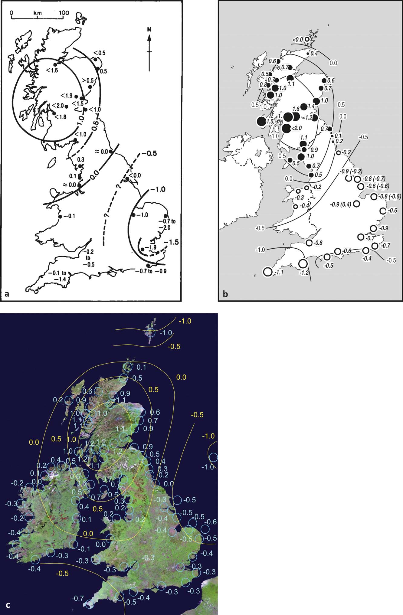
Figure 5 Evolution of patterns of Late Holocene glacial isostatic adjustment in mm yr–1 for the British Isles, modelled using geological sea-level reconstructions: (a) crustal movements, constrained with data since 8800 BP. Copyright (1989) Wiley. Used with permission from Shennan, I., Holocene crustal movements and sea-level changes in Great Britain, Journal of Quaternary Science, John Wiley & Sons (License Number 3758450488920); (b) relative land-/ sea-level changes from data since 4000 cal yr BP. Copyright (2002) Wiley. Used with permission from Shennan, I. & Horton, B., Holocene land- and sea-level changes in Great Britain, Journal of Quaternary Science, John Wiley & Sons (License Number 3758460787033); (c) relative land-/ sea-level changes from data since 1000 BP, with a centre of relative land uplift (positive values) over northern Scotland and three sub-centres of relative subsidence (negative values) over southwest England, the southern North Sea and the Shetland Isles. Copyright (2012) Wiley. Used with permission from Shennan, I., Milne, G. & Bradley, S. L., Late Holocene vertical land motion and relative sea-level changes: lessons from the British Isles, Journal of Quaternary Science, John Wiley & Sons (License Number 3758461230828).
Shennan et al. (Reference Shennan, Milne and Bradley2012) provided a revised map of late Holocene relative land- and sea-level rates, based on the recent GIA modelling advances (Shennan et al. Reference Shennan, Bradley, Milne, Brooks, Bassett and Hamilton2006a; Brooks et al. Reference Brooks, Bradley, Edwards, Milne, Horton and Shennan2008; Bradley et al. Reference Bradley, Milne, Shennan and Edwards2011) constrained by geological sea-level indicators. Reference ArgusFigure 5c displays the centre of relative uplift again over central Scotland due to GIA; however, the areas of relative subsidence are more differentiated, with three sub-centres over southwest England, the southern North Sea and the Shetland Isles, demonstrating other governing factors, including ocean loading as well as far-field GIA signals. Furthermore, in contrast to 2002, the value of the relative uplift of Scotland is again lower in the 2012 results, with correspondingly reduced rates of relative subsidence in England. Those differences can be explained by an increase in observational data, improvement of the models and further consideration of sediment compaction (Shennan et al. Reference Shennan, Milne and Bradley2009, Reference Shennan, Milne and Bradley2012).
By comparison, the results within the second school of thought of Holocene RSL research (Smith et al. Reference Smith, Fretwell, Cullingford and Firth2006, Reference Smith, Hunt, Firth, Jordan, Fretwell, Harman, Murdy, Orford and Burnside2012) show a similar spatial pattern of relative sea-level changes, based on shoreline altitude measurements and Gaussian Quadratic Trend Surface isobase modelling. The prominent shorelines shown in Reference Argus, Peltier and WatkinsFigure 6 are a result of relative stability of vertical land motion and RSL changes. The Main Postglacial Shoreline emerges as the highest one in the uplift centre of Scotland, with 10 m relative to MHWS (mean high water ordinary spring tides). The Blair Drummond Shoreline is the second highest shoreline, with 8 m MHWS, followed by the Wigtown Shoreline with 6 m MHWS, which is the youngest and lies on top of other shorelines at the margins of Scotland. The Storegga Shoreline is located below the other shorelines, with 4 m MHWS at its maximum altitude (Smith et al. Reference Smith, Hunt, Firth, Jordan, Fretwell, Harman, Murdy, Orford and Burnside2012).

Figure 6 Spatial pattern of RSL change during the Holocene as indicated by the Storegga (A), Main Postglacial (B), Blairdrummond (C) and Wigtown (D) shorelines (chronologically ordered), based on Gaussian Quadratic Trend Surface modelling and constrained to a common axis and centre in the southeast Grampian Highlands of Scotland. Displayed are heights above MHWS with location of altitudinal data points (circles). The greater the distance from the centre of uplift in central Scotland, the more visible the younger shorelines become on the surface. Reprinted from Quaternary Science Reviews 54, Smith, D. E., Hunt, N., Firth, C. R., Jordan, J. T., Fretwell, P. T., Harman, M., Murdy, J., Orford, J. D. & Burnside, N. G., Patterns of Holocene relative sea level change in the North of Britain and Ireland, 58–76. Copyright (2012), with permission from Elsevier (License Number 3767110438627).
3. Geodetic measurement techniques and GIA modelling
Geodetic measurements provide a second broad type of data to quantify crustal motion and hence potentially to constrain GIA model parameters or to correct sea-level trends at tide gauges. These geodetic measurements are of present (vertical) crustal motion over monthly, annual and perhaps decadal timescales, and their relationship to, and consistency with, the quantification of GIA using geological information on sea-level change has yet to be fully assessed.
Geodesy is a powerful tool for monitoring crustal motions worldwide; however, detecting vertical movement often presents more of a challenge due to its magnitude of about 1–10 mm yr–1, compared to horizontal tectonic movement of about 1–15 cm yr–1 (Soudarin et al. Reference Soudarin, Crétaux and Cazenave1999). Space-based, airborne or ground-based methods, such as very long baseline interferometry (VLBI), measurements of the gravity field, global navigation satellite systems (GNSS), sattelite laser ranging (SLR) or Doppler orbitography and radio positioning integrated by satellite (DORIS), and a combination thereof, have shown potential to produce (direct) estimates of present-day vertical land motion (VLM) and, thereby, to quantify GIA rates (e.g., Ashkenazi et al. Reference Ashkenazi, Bingley, Whitmore and Baker1993; James & Lambert Reference James and Lambert1993; Mitrovica et al. Reference Mitrovica, Davis and Shapiro1993; Peltier Reference Peltier1995; Argus Reference Argus1996; Argus et al. Reference Argus, Peltier and Watkins1999; Larson & van Dam Reference Larson and van Dam2000; Lambert et al. Reference Lambert, Courtier, Sasagawa, Klopping, Winester, James and Liard2001; Hill et al. Reference Hill, Davis, Tamisiea and Lidberg2010).
With respect to northern Britain, the DORIS, SLR and VLBI techniques suffer from limitations in vertical resolution, since their networks are too sparse and their stations too far away from the centre of postglacial rebound in Scotland to be sensitive to the GIA signal. Thus, for the British Isles, the main geodetic techniques applied for measuring VLM are absolute gravimetry (AG) and continuous GPS (CGPS). Those estimates are often used for the correction of tide gauge records to derive climate-induced sea-level change, by removing the vertical land motion component from the relative sea-level trends.
3.1. Point measurements of crustal motions
3.1.1. Absolute gravimetry
Gravity measurements have been used in the past to quantify various geodynamic processes that have influence on the gravitational field on different spatial and temporal scales, from ocean tides and groundwater changes to sea-level changes, plate boundary deformation and long-term postglacial rebound (Lambert et al. Reference Lambert, Courtier and James2006). Gravimetry is a valuable geodetic observation tool that contributes to the precise definition of a common Geoid, a global reference system and explanation of geodynamic processes. Gravitational field measurements can be taken both from space (e.g., Gravity Recovery and Climate Experiment – GRACE; or ESA's Gravity Field and Steady-State Ocean Circulation Explorer – GOCE) and in terrestrial approaches (e.g., stationary absolute gravimeters) for mass redistributions in, for example, the mantle of the Earth in response to glacial rebound. As well as in the British Isles, these measurements have been applied in several other glacial rebound areas, such as Laurentia (Lambert et al. Reference Lambert, Courtier, Sasagawa, Klopping, Winester, James and Liard2001; Tamisiea et al. Reference Tamisiea, Mitrovica and Davis2007) and Fennoscandia (Hill et al. Reference Hill, Davis, Tamisiea and Lidberg2010).
For the UK, Williams et al. (Reference Williams, Baker and Jeffries2001) presented some preliminary results for the absolute gravity technique for three tide gauges for a 3–4-year measurement period, beginning in Newlyn and Aberdeen in 1995 and in Lerwick in 1996. Gravity is measured by dropping a test mass, a corner-cube retroflector, in a vacuum. This happens every ten seconds, while measurements by an iodine-stabilised He–Ne laser interferometer, together with a rubidium atomic clock, allow the equations of motion for acceleration of the mass to be solved (Niebauer et al. Reference Niebauer, Sasagawa, Faller, Hilt and Klopping1995; Williams et al. Reference Williams, Baker and Jeffries2001; Teferle et al. Reference Teferle, Bingley, Waugh, Dodson, Williams, Baker, Tregoning and Rizos2007). Measurements are taken, for instance, every year for 3–4 days at each site. The sites are located on stable bedrock, and regular inter-comparisons with other gravimeters in Europe and the USA allow a consistently good accuracy within 1–2 μGal to be maintained (Williams et al. Reference Williams, Baker and Jeffries2001). Today's accuracy of gravity measurements is about 10–9 g (1 μGal or 10 nm/s2), which translate to height changes of about 3 mm relative to the Earth centre of mass (Forsberg et al. Reference Forsberg, Sideris and Shum2005; Blewitt et al. Reference Blewitt, Altamimi, Davis, Gross, Kuo, Lemoine, Moore, Neilan, Plag, Rothacher, Church, Woodworth, Aarup and Wilson2010). It is possible to find different ratios between gravity change rates and vertical displacement rates (for the conversion of gravity values to vertical land motion) in the literature, but Williams et al. (Reference Williams, Baker and Jeffries2001) assume that a change in gravity of 0.2 μGal is associated with a height change of 1 mm. Results show vertical land motion of 1.0±1.4 mm yr–1 at Newlyn, southwest England, −3.8±1.6 mm yr–1 at Lerwick, Shetland and 0.9±3.1 mm yr–1 at Aberdeen, Scotland, mostly reflecting the general glacio-isostatic pattern in the UK.
3.1.2. Continuous GNSS
The use of global navigation satellite systems (GNSS), and especially a global positioning system (GPS), is widely applied for direct measurements of surface displacement and vertical crustal motions of the British Isles. The technique of continuous GPS measurements is frequently used near tide gauge stations to derive the vertical station velocities from height coordinate time-series. A high precision of more than 1 mm yr–1 can be achieved with this technique, using a few years of observations (Blewitt et al. Reference Blewitt, Altamimi, Davis, Gross, Kuo, Lemoine, Moore, Neilan, Plag, Rothacher, Church, Woodworth, Aarup and Wilson2010). The advantages of using GPS at tide gauges were recognised as early as 1990, with episodic GPS in the UK following recommendations of Carter et al. (Reference Carter, Aubrey, Baker, Boucher, LeProvost, Pugh, Peltier, Zumberge, Rapp and Schultz1989). Subsequently, the Institute of Engineering Surveying and Space Geodesy (IESSG) and the Proudman Oceanographic Laboratory (POL) implemented several campaigns (Bingley et al. Reference Bingley, Dodson, Penna, Teferle and Baker2001). Early studies on determining GPS station heights in the UK, and testing their accuracy, were undertaken, for example, by Ashkenazi et al. (Reference Ashkenazi, Bingley, Whitmore and Baker1993). The importance of permanent measurements in the form of continuous GPS (CGPS) at tide gauges was emphasised in 1993 by the International Association for Physical Sciences of the Ocean (IAPSO) Committee (Carter Reference Carter1994). The number of CGPS stations worldwide has increased rapidly since 1993, in conjunction with increasingly cheaper GPS receivers and better computer hardware and software, with the main purpose of realising the International Terrestrial Reference System (the newest one being the ITRF2008, with ITRF2014 under preparation). In the UK, the establishment of CGPS stations at tide gauges by IESSG and POL, for the measurement of VLM, commenced in 1997 (Teferle et al. Reference Teferle, Bingley, Williams, Baker and Dodson2006). Today, around 160 operating CGPS stations can be found UK-wide, according to the UK Ordnance Survey. The application of CGPS in conjunction with absolute gravity measurements has been implemented by IESSG and POL since the late 1990s in the UK, with the establishment of three AG stations in the proximity of tide gauges (Teferle et al. Reference Teferle, Bingley, Waugh, Dodson, Williams, Baker, Tregoning and Rizos2007).
Permanent GPS observations have also been extensively used in Fennoscandia, mostly in large-scale campaigns within the BIFROST (Baseline Inferences for Fennoscandian Rebound Observations, Sea-Level and Tectonics) project (Milne et al. Reference Milne, Davis, Mitrovica, Scherneck, Johansson, Vermeer and Koivula2001, Reference Milne, Mitrovica, Scherneck, Davis, Johansson, Koivula and Vermeer2004; Johansson et al. Reference Johansson, Davis, Scherneck, Milne, Vermeer, Mitrovica, Bennett, Jonsson, Elgered, Elosegui, Koivula, Poutanen, Ronnang and Shapiro2002; Lidberg et al. Reference Lidberg, Johansson, Scherneck and Davis2007). GPS benefits from the fact that receivers are based on the ground and not on the satellite. Thus, the receivers can be used more flexibly at different locations. GPS equipment has also become increasingly cheaper and, with a range of scientific-quality software packages available, the processing of GPS observations is more accessible. CGPS stations can be set up directly at tide gauge locations, thus being representative of the VLM at that station, excluding other deformation effects from surrounding areas. The direct link with the International Terrestrial Reference Frame (ITRF) theoretically allows tide gauge benchmarks to be connected via a common global reference frame and, thus, making comparisons of sea-level datasets possible (Wöppelmann et al. Reference Wöppelmann, Zerbini and Marcos2006). However, it has to be considered that several external and internal GPS error sources can introduce biases in station time-series and velocities, especially in the vertical component, leading to increased scatter and higher uncertainty compared to the horizontal components. Creating false signals in the GPS estimates, such error sources are, for example:
• variations in the phase centres of satellite and receiver antennas;
• ionospheric and tropospheric delays and mis-modelling thereof in the processing;
• atmosphere, ocean and surface hydrologic loading;
• uncertainties in satellite orbits;
• multipath due to reflection from surrounding objects;
• satellite and receiver clock errors;
• unaccounted geophysical processes;
• unfavourable satellite constellation leading to dilution of precision;
• realisation or constraints of the reference frame applied.
For geophysical analysis, GPS observation periods should be at least 2.5 years in length, to allow estimation of annual and semi-annual signals and obtain realistic velocity estimates (Blewitt & Lavallée Reference Blewitt and Lavallée2002).
For the UK, Bingley et al. (Reference Bingley, Dodson, Penna, Teferle and Baker2001) presented some preliminary results from episodic GPS (EGPS) campaigns between 1991 and 1996, combined with the first five continuous GPS stations (Sheerness, Newlyn, Aberdeen, Liverpool and Lowestoft), and gave a first impression of the magnitude of VLM at tide gauges, which corresponds to results derived from long-term relative sea-level observations in Woodworth et al. (Reference Woodworth, Tsimplis, Flather and Shennan1999) in the range of 0–3 mm yr–1. Sanli & Blewitt (Reference Sanli and Blewitt2001) analysed the tide gauge North Shields in northeast England in terms of VLM, derived from a single GPS campaign directly tied to the tide gauge benchmark. They evaluated GPS as an alternative method to the use of GIA models for the correction of sea-level trends and confirmed its capability to derive independent estimates of sea-level change. The VLM at the station accounted for 0.6±1.5 mm yr–1, with an associated geocentric sea-level rise of 2.6±1.0 mm yr–1. Considering that the tide gauge measurement alone (1.8 mm yr–1) would have underestimated geocentric sea-level rise, they emphasised the importance of correcting tide gauge records for postglacial rebound.
Concentrating on refining GPS methodology, Teferle et al. (Reference Teferle, Bingley, Dodson and Baker2002) tested the method of using dual-continuous GPS stations for monitoring vertical land motion at tide gauges. This involves one GPS directly at the tide gauge, which measures the actual VLM of this station, and another one within a range of a few kilometres on stable bedrock, which allows the separation of short-term motions of the tide gauge structure itself from underlying geophysical processes. This concept for long-term station velocity monitoring had already been mentioned by Bingley et al. (Reference Bingley, Dodson, Penna, Teferle and Baker2001) and was originally proposed by Plag et al. (Reference Plag, Axe, Knudsen, Richter and Verstraeten2000). With the dual-CGPS concept, Teferle et al. (Reference Teferle, Bingley, Dodson and Baker2002) addressed the known issue of biases in coordinate time-series caused by temporal or spatial correlations. Their approach facilitates the removal of those systematic effects, which are common to both time-series, by differencing the coordinate time-series of both stations and, thus, obtaining a coordinate time-series with fewer systematic biases.
3.1.3. Continuous GPS combined with absolute gravimetry
The common biases that result in loss of accuracy and precision in CGPS can be addressed by using spatial filtering techniques that effectively limit parameter uncertainty (e.g., Wdowinski et al. Reference Wdowinski, Bock, Zhang, Fang and Genrich1997; Johansson et al. Reference Johansson, Davis, Scherneck, Milne, Vermeer, Mitrovica, Bennett, Jonsson, Elgered, Elosegui, Koivula, Poutanen, Ronnang and Shapiro2002; Dong et al. Reference Dong, Fang, Bock, Webb, Prawirodirdjo, Kedar and Jamason2006). Among the possible reasons for the systematic biases in GPS estimates named above are errors in the International Terrestrial Reference Frame (ITRF), which influence vertical station velocity (Altamimi et al. Reference Altamimi, Collilieux, Legrand, Garayt and Boucher2007, Reference Altamimi, Collilieux and Métivier2011). The accuracy of CGPS depends heavily on the accuracy of the ITRF, and difficulties remain in determining the geocentre of the ITRF and its motion relative to the Earth's centre of mass (Blewitt Reference Blewitt2003; Dong et al. Reference Dong, Yunck and Heflin2003; Teferle et al. Reference Teferle, Bingley, Waugh, Dodson, Williams, Baker, Tregoning and Rizos2007, Reference Teferle, Bingley, Orliac, Williams, Woodworth, McLaughlin, Baker, Shennan, Milne and Bradley2009).
Absolute gravity (AG) measurements of VLM, however, show good accuracy in general, since those kinds of biases are missing here. AG is independent of the ITRF (Teferle et al. Reference Teferle, Bingley, Orliac, Williams, Woodworth, McLaughlin, Baker, Shennan, Milne and Bradley2009). Thus, AG measurements can help assess CGPS estimates of vertical land motion. The issue with the accuracy of CGPS measurements (systematic offsets from other observation techniques) has been dealt with by Teferle et al. (Reference Teferle, Bingley, Williams, Baker and Dodson2006, Reference Teferle, Bingley, Waugh, Dodson, Williams, Baker, Tregoning and Rizos2007), for instance, by aligning the CGPS estimates with AG measurements. For nine tide gauges in the UK and northern France, these authors demonstrated how the integration of the two techniques can contribute to more reliable estimates of the vertical station velocities using time-series, starting in 1997 for CGPS and 1995/96 for AG. They compared alternatives to their CGPS/AG method for deriving vertical land motion, including: (1) using geological evidence; (2) using the inverse of the difference between the mean sea-level trend at British tide gauges and an assumed absolute sea-level rise of 1.5 mm yr–1 for northern Europe (see also Woodworth et al. Reference Woodworth, Tsimplis, Flather and Shennan1999); and (3) using GIA models. They pointed out a systematic offset between CGPS estimates on the one hand and the AG estimates, as well as those other independent estimates of VLM, on the other hand. Other authors have also found a systematic offset between CGPS and the outputs of AG, GIA models and very long baseline interferometry measurements for stations in Europe and North America, with CGPS generally being more positive. The causes lie within the GPS processing chain (antenna phase centre modelling, reference frame realisation, etc.) (Teferle et al. Reference Teferle, Bingley, Orliac, Williams, Woodworth, McLaughlin, Baker, Shennan, Milne and Bradley2009).
The AG-alignment encompasses a calculation of the offset between the CGPS and AG-based VLM estimates, which account for 1.2±0.4 mm yr–1 (Teferle et al. Reference Teferle, Bingley, Waugh, Dodson, Williams, Baker, Tregoning and Rizos2007), and which is consistent with the offset between CGPS and other independent techniques, as well as with values found in the literature (MacMillan Reference MacMillan2004; Prawirodirdjo & Bock Reference Prawirodirdjo and Bock2004). In a next step, the weighted mean difference between the vertical station velocity estimates from CGPS and AG is calculated and afterwards subtracted from the CGPS estimates, which results in the AG-aligned CGPS estimates of vertical crustal motions (Hansen et al. Reference Hansen, Teferle, Bingley, Williams, Kenyon, Pacino and Marti2012). Results of those estimates of vertical station velocity in Teferle et al. (Reference Teferle, Bingley, Waugh, Dodson, Williams, Baker, Tregoning and Rizos2007) lead to a de-coupled absolute sea-level rise of about 1.3±0.3 mm yr–1 around the British Isles. But due to remaining uncertainties in the CGPS and AG time-series, the statistical significance of these results could not yet be established.
Teferle et al. (Reference Teferle, Bingley, Orliac, Williams, Woodworth, McLaughlin, Baker, Shennan, Milne and Bradley2009) extended this survey and compared the results of different independent CGPS processing strategies, including the effects of spatial filtering and reference frame implementations for deriving CGPS and AG-aligned CGPS estimates of present-day vertical, as well as horizontal, crustal motion. Their two processing strategies involved: (1) a daily double-difference (DD) regional network (RN) solution, produced from 1997 to 2005 (DDRN); and (2) a series of daily precise point positioning (PPP) globally transformed (GT) solutions from 2000 to 2005 (PPPGT). In the first approach, a regional reference frame with four European IGS (International GNSS Service) stations within the ITRF2000 was implemented. The second processing strategy used a globally extended reference frame with the 99 IGS stations within the IGS realisation of the ITRF2000. Additionally, they compared filtered and unfiltered results with regard to spatial correlation in the time-series. For validation purposes, they used derivations of vertical crustal motion based on the Holocene geological information on relative sea-level trends from Shennan & Horton (Reference Shennan and Horton2002) and Shennan et al. (Reference Shennan, Hamilton, Hillier, Hunter, Woodall, Bradley, Milne, Brooks and Bassett2006b). Teferle et al. (Reference Teferle, Bingley, Orliac, Williams, Woodworth, McLaughlin, Baker, Shennan, Milne and Bradley2009) concluded that a simultaneous processing using two or more independent CGPS processing solutions is important to get the best possible, or most realistic results, from station data. They showed that geodetic techniques complement each other and that an independent data set for validation, such as geological information, is crucial.
Reference Argus, Heflin, Peltzer, Crampé and WebbFigure 7 shows their results and differences between CGPS only (Reference Argus, Heflin, Peltzer, Crampé and WebbFig. 7a, b) and AG-aligned CGPS (Reference Argus, Heflin, Peltzer, Crampé and WebbFig. 7c, d) estimates of vertical station velocity for Great Britain for the two CGPS processing solutions DDRNF and PPPGTF. Those geodetic results of present-day crustal motions confirm the general trend of the geological map of Holocene data (see Reference ArgusFig. 5), which is subsidence in the area of Shetland and in most of England and Wales, and uplift in most areas of Scotland. Offsets in vertical station velocities between DDRNU and PPPGTU account for 1.1±1.1 mm yr–1, and 0.7±0.6 mm yr–1 between DDRNF and PPPGTF (regional vs. global reference frame realisation). Those offsets between processing strategies could again be significantly reduced with AG-alignment. The systematic offsets between AG and CGPS are stated as 1.5 mm yr–1 and 1.3 mm yr–1 for DDRNU and DDRNF respectively relative to AG, and 0.6 mm yr–1 for both PPPGTU and PPPGTF relative to AG, with the CGPS estimates being more positive in all cases. As the maps show, the geodetic results vary significantly between each other in spatial distribution and magnitude of the vertical land motion shown, depending on what CGPS processing strategy (with regional or global reference frame implementations) has been used, or whether AG-alignment has been performed.
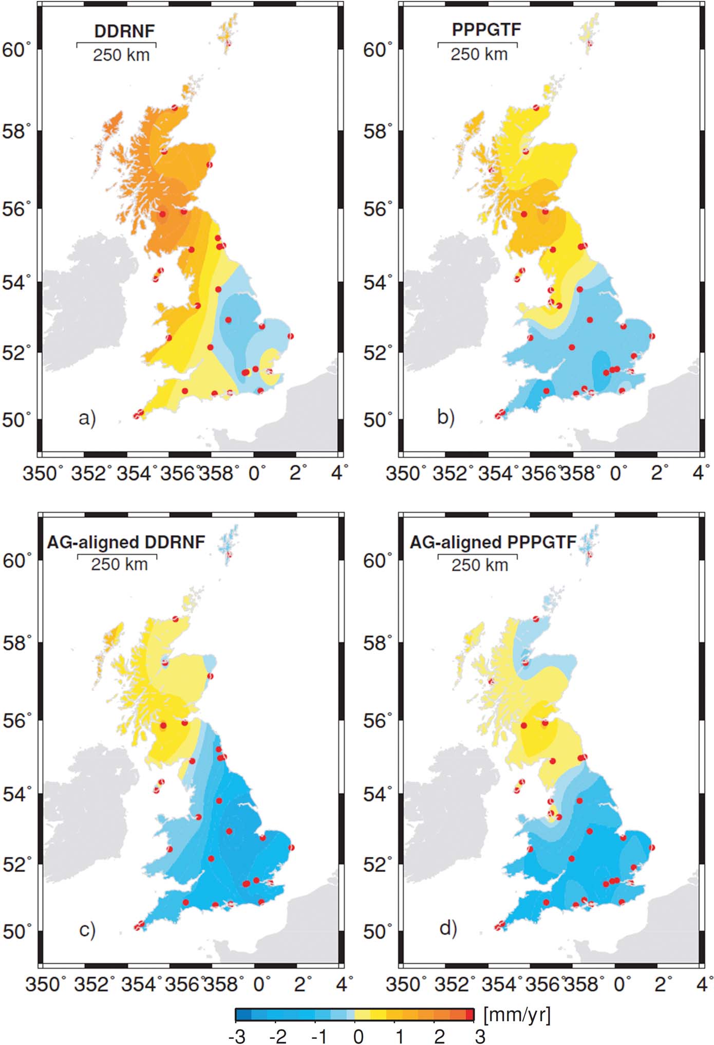
Figure 7 Vertical crustal motions in Great Britain from CGPS (a, b) and AG-aligned CGPS (c, d) estimates for two CGPS processing techniques: DDRNF denotes a series of daily double-difference (DD) regional network (RN) solutions, while PPPGTF stands for a series of daily precise point positioning (PPP) globally transformed (GT) solutions. Processing time frame: 1997–2005. F means spatial filtering. Red dots represent CGPS stations. Reproduced from: Teferle, F. N., Bingley, R. M., Orliac, E. J., Williams, S. D. P., Woodworth, P. L., McLaughlin, D., Baker, T. F., Shennan, I., Milne, G. A. & Bradley, S. L., Crustal motions in Great Britain: evidence from continuous GPS, absolute gravity and Holocene sea level data, Geophysical Journal International, 2009, 178, 1, 23–46, by permission of Oxford University Press, published on behalf of the Royal Astronomical Society.
Hansen et al. (Reference Hansen, Teferle, Bingley, Williams, Kenyon, Pacino and Marti2012) presented an update on present-day vertical land motion in the UK from CGPS and AG-aligned CGPS measurements. In contrast to the results of Teferle et al. (Reference Teferle, Bingley, Orliac, Williams, Woodworth, McLaughlin, Baker, Shennan, Milne and Bradley2009), stations in Northern Ireland are included, which allows the definition of the western boundary of uplift due to GIA in the north of the UK (see Reference Arıkan, Hooper, Hanssen and Lacoste-FrancisFig. 8b, compared to Reference Argus, Heflin, Peltzer, Crampé and WebbFig. 7). A re-processing of the BIGF (British Isles continuous GNSS facility) network (daily double-differenced solutions within a semi-global reference frame realisation, ITRF2005, of 37 IGS stations) for the period between 1997 and 2008 involved a re-assessment of the stations that are representative of crustal motion, by analysing surface and bedrock geological data, site photographs and monumentation data, and an exclusion of stations with time-series lengths of less than six years. For Scotland, where continuous measurement periods were mostly shorter than that, the dual-CGPS approach of Teferle et al. (Reference Teferle, Bingley, Dodson and Baker2002) was applied. Thus, 46 stations across the UK were determined as appropriate for geophysical research (Hansen et al. Reference Hansen, Teferle, Bingley, Williams, Kenyon, Pacino and Marti2012).
Additional to the maps from 2005 (Teferle et al. Reference Teferle, Bingley, Orliac, Williams, Woodworth, McLaughlin, Baker, Shennan, Milne and Bradley2009) and from 2008 (Hansen et al. Reference Hansen, Teferle, Bingley, Williams, Kenyon, Pacino and Marti2012), other AG-aligned CGPS maps of current vertical crustal uplift have been published, a few of which are presented in Reference Arıkan, Hooper, Hanssen and Lacoste-FrancisFigure 8. Generally, more and more stations have been included over the years, since the observation period per station has become longer and many new stations now fulfil the minimal time-frame requirement. When comparing the maps, it is important to keep in mind the different reference frame implementations and subsets or regional realisations thereof (ITRF2000, ITRF2005, ITRF2008, IGb08, etc.), as they are likely to cause offsets between the maps. A shift of the uplift centre's location within Scotland is noticeable. It is difficult to define this clearly, as it depends on the applied processing strategy or the amount of total stations included, amongst other factors. In Teferle et al. (Reference Teferle, Bingley, Orliac, Williams, Woodworth, McLaughlin, Baker, Shennan, Milne and Bradley2009) the maximum uplift tends towards the east for the PPPGTF solution, with 1.6±0.3 mm yr–1 in Edinburgh (1.1±0.3 mm yr–1 AG-aligned). In Bradley et al. (Reference Bradley, Milne, Teferle, Bingley and Orliac2009) (Reference Arıkan, Hooper, Hanssen and Lacoste-FrancisFig. 8a), it is visibly located in eastern Scotland, with 1.07±0.35 mm yr–1 in Edinburgh. The processing of this data considered motion relative to the station in Sheerness in southeast England. Hansen et al. (Reference Hansen, Teferle, Bingley, Williams, Kenyon, Pacino and Marti2012) included data from Ireland and the uplift centre shifts towards western Scotland, similar to the BIGF map from 2010 (Reference Arıkan, Hooper, Hanssen and Lacoste-FrancisFig. 8b, c). This is more consistent with GIA model outputs. The BIGF map from Reference Hansen and Bingley2015 (Reference Arıkan, Hooper, Hanssen and Lacoste-FrancisFig. 8d) places it again more towards central/eastern Scotland, and shows a spatially more diverse pattern, with the increasing number of stations included. For example, highest values are found in DRUM (1.43±0.36 mm yr–1), EDIN (1.38±0.23 mm yr–1), KILN (1.30±0.39 mm yr–1) and BRAE (1.30 ± 0.42 mm yr–1) (BIGF Reference Hansen and Bingley2015).
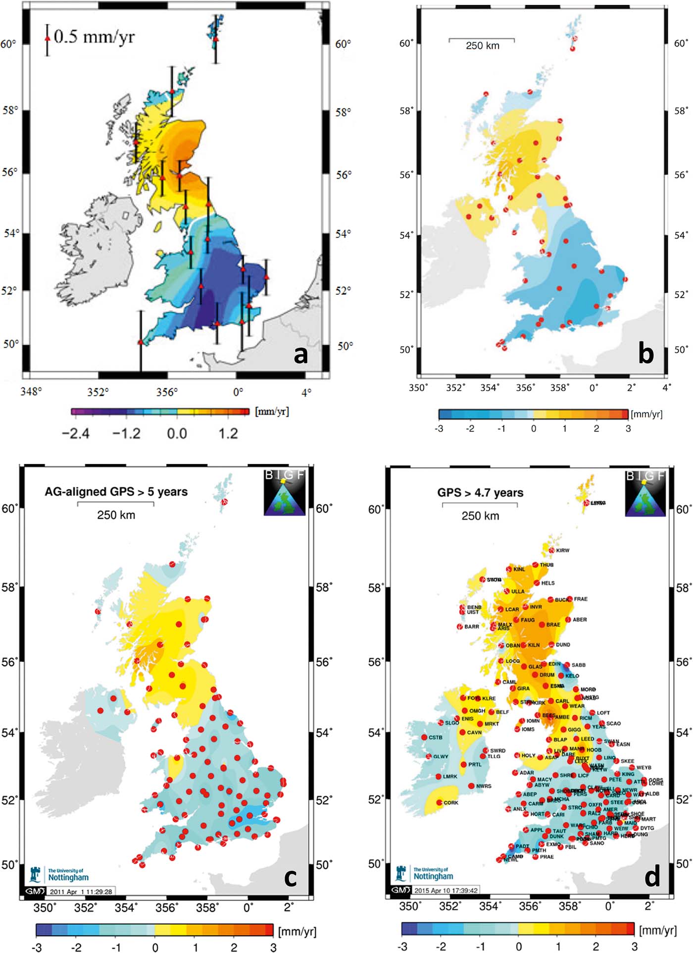
Figure 8 Comparison of maps of vertical land motion derived from AG-aligned CGPS station measurements in The British Isles (stations indicated by red dots). They differ in processing time-frame, amount of included CGPS receivers, reference frame implementation and minimum time-series duration: (a) processing time frame 1997–2005, 16 CGPS sites, motion calculated relative to station in Sheerness, >4 years minimum time-series duration. Reproduced from: Bradley, S. L., Milne, G. A., Teferle, F. N., Bingley, R. M. & Orliac, E. J., Glacial isostatic adjustment of the British Isles: new constraints from GPS measurements of crustal motion, Geophysical Journal International, 2009, 178, 14–22, by permission of Oxford University Press, published on behalf of the Royal Astronomical Society; (b) 1997–2008, 46 CGPS sites, semi-global reference frame implementation with 37 IGS stations within ITRF2005, >6 years minimum time-series duration. Reproduced from: Geodesy for Planet Earth 2012, 665-671, New estimates of resent-day crustal/land motions in the British Isles based on the BIGF network, Hansen, D. N., Teferle, F. N., Bingley, R. M. & Williams, S. D. P., Figure 82.5b, with permission from Springer Science+Business Media (License Number 378141019339); (c) 1997–2010, 104 CGPS sites, global reference frame network within ITRF2008, >5 years. Reproduced from Greaves et al. (Reference Greaves, Bingley, Baker, Hansen, Sherwood and Clarke2013), with permission from British Isles continuous GNSS Facility (BIGF); (d) 1997–2015, 158 CGPS sites, global reference frame implementation, IGb08, >4.7 years. Reproduced from Greaves et al. (Reference Greaves, Bingley, Baker, Hansen and Clarke2015), with permission from BIGF.
Such geodetically derived comprehensive data sets of present-day vertical crustal motions of the British Isles provide the data basis (horizontal and vertical station velocity estimates) for further studies; including the work of Woodworth et al. (Reference Woodworth, Teferle, Bingley, Shennan and Williams2009), who estimated rates of mean sea-level change around the UK from tide gauges, and that of Milne et al. (Reference Milne, Shennan, Youngs, Waugh, Teferle, Bingley, Bassett, Cuthbert-Brown and Bradley2006) and Bradley et al. (Reference Bradley, Milne, Teferle, Bingley and Orliac2009, Reference Bradley, Milne, Shennan and Edwards2011), who concentrated on the improvement of GIA models using CGPS data for further parameter constraint. The latter technique is elaborated in more detail in the next section.
3.2. GIA modelling approaches with parameter constraints from CGPS
GIA modelling studies (e.g., Lambeck Reference Lambeck1993a, Reference Lambeckb; Shennan et al. Reference Shennan, Lambeck, Horton, Innes, Lloyd, McArthur, Purcell and Rutherford2000, Reference Shennan, Peltier, Drummond and Horton2002; Peltier et al. Reference Peltier, Shennan, Drummond and Horton2002) produced good overall results for the pattern of general relative sea-level (RSL) change, but they failed to provide good fits at all observation sites, and tended to underestimate the extremes of RSL change observations (Shennan & Horton Reference Shennan and Horton2002). With the emergence and refinement of the CGPS technology, several attempts at modelling glacial rebound have been undertaken, which include both the geological Holocene RSL evidence and the information gained from CGPS measurements to constrain modelling parameters. With this new data source, the aim is now no longer to reproduce Holocene RSL curves, but rather use the GIA models (calibrated with Holocene sea-level evidence) to predict today's short-term vertical land motion, for which CGPS observations give important clues for further parameterisation.
The most obvious contribution of CGPS data to GIA modelling is that CGPS provides information from spatially more evenly distributed observation points, as well as about the UK's interior, while RSL indicators were limited to the coast.
Milne et al. (Reference Milne, Mitrovica, Scherneck, Davis, Johansson, Koivula and Vermeer2004, Reference Milne, Shennan, Youngs, Waugh, Teferle, Bingley, Bassett, Cuthbert-Brown and Bradley2006) utilised the advantage that CGPS gives information about three-dimensional crustal motions, including the horizontal velocity field induced by GIA, whereas sea-level data can only provide indirect measurements of vertical movement. They validated the present-day model predictions of horizontal crustal motion of GIA against the CGPS observations of 12 stations in the UK. These authors aimed to address the weaknesses of previous GIA models (Lambeck Reference Lambeck1993a, Reference Lambeckb; Peltier et al. Reference Peltier, Shennan, Drummond and Horton2002; Shennan et al. Reference Shennan, Peltier, Drummond and Horton2002), such as the risk of overestimation of the ice thickness in regions with high terrain, such as northwest Scotland, since the earlier applied ice-models had assumed a flat topography underneath the ice layer. They found that, previously, the ice thickness had been overestimated by up to 500 m, and that now, with terrain-correction, the model fit could be improved. They also endorsed a rather rapid ice growth phase, culminating in the Last Glacial Maximum. Therefore, Peltier et al. (Reference Peltier, Shennan, Drummond and Horton2002) (who assumed an equilibrium ice sheet before the LGM) had overestimated vertical deformation after deglaciation. However, the study of Milne et al. (Reference Milne, Shennan, Youngs, Waugh, Teferle, Bingley, Bassett, Cuthbert-Brown and Bradley2006) also demonstrated the emergence of new modelling difficulties, while trying to achieve a good fit of the GIA model to both the RSL and the CGPS data.
Bradley et al. (Reference Bradley, Milne, Teferle, Bingley and Orliac2009) extended Milne's et al. (Reference Milne, Shennan, Youngs, Waugh, Teferle, Bingley, Bassett, Cuthbert-Brown and Bradley2006) study by examining the information content of the entire 3D-velocity field of the GIA component in Great Britain, introducing the vertical GPS deformation information (see Reference Arıkan, Hooper, Hanssen and Lacoste-FrancisFig. 8a), since the time-series were now long enough to reach the required accuracy for the vertical coordinate. They tried to analyse the measured and modelled vertical land motion component that is caused by the British–Irish ice sheet alone, thus using relative CGPS deformation values between the station in Sheerness and the rest of the UK, and eliminating the influence from far-field ice sheets. Reference Ashkenazi, Bingley, Whitmore and BakerFigure 9 illustrates the two components of the complete modelled signal of present-day land uplift (Reference Ashkenazi, Bingley, Whitmore and BakerFig. 9a), after decomposition into the signal from the non-local ice sheets (Reference Ashkenazi, Bingley, Whitmore and BakerFig. 9b) and from the British–Irish ice sheet and ocean (Reference Ashkenazi, Bingley, Whitmore and BakerFig. 9c). It shows the subsidence for all of the British Isles caused by the Fennoscandian ice sheet with a magnitude of more than 1 mm yr–1. The general pattern of the total current vertical land motion signal is consistent with the spatial distribution of relative motion in previous modelling results of Late Holocene RSL change (see Reference ArgusFig. 5), with an SSW–NNE oriented ellipse of an upward trend in Scotland and North Ireland, with the centre in central western Scotland and subsidence in most of England.
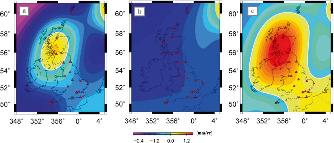
Figure 9 (a) Modelled current rates of land uplift (5 km×5 km grid) from model constrained by both geological sea-level observations and AG-aligned CGPS estimates. (b, c) Decomposed total signal of (a): (b) showing the effects of non-local ice sheets; (c) showing effects of British–Irish ice sheet and ocean loading only. Reproduced from: Bradley, S. L., Milne, G. A., Teferle, F. N., Bingley, R. M. & Orliac, E. J., Glacial isostatic adjustment of the British Isles: new constraints from GPS measurements of crustal motion, Geophysical Journal International, 2009, 178, 14–22, by permission of Oxford University Press, published on behalf of the Royal Astronomical Society.
Despite encountering the parameter trade-off problem again, Bradley et al. (Reference Bradley, Milne, Teferle, Bingley and Orliac2009) found that the CGPS data provided a robust constraint for the upper mantle viscosity, and thus suggested that an integration of Holocene sea-level and modern CGPS data would better constrain the viscosity structure model of the Earth.
Bradley et al. (Reference Bradley, Milne, Shennan and Edwards2011) presented the latest study in GIA modelling for the British Isles, drawing upon a variety of constraints from several previous studies: Bradley et al. (Reference Bradley, Milne, Teferle, Bingley and Orliac2009) for the constraint of the Earth-model viscosity values from the CGPS data; Shennan et al. (Reference Shennan, Bradley, Milne, Brooks, Bassett and Hamilton2006a) and Brooks et al. (Reference Brooks, Bradley, Edwards, Milne, Horton and Shennan2008) for the British–Irish ice component of the model, based on an integration of geomorphological field constraints from both Great Britain and introducing Ireland; and a non-local/global ice-model combined from Bassett et al. (Reference Bassett, Milne, Mitrovica and Clark2005) and Bradley et al. (Reference Bradley, Milne, Zong and Horton2008), the latter extending the melting period further into the Holocene with far-field RSL data for the prediction of eustatic sea-level change. Bradley et al. (Reference Bradley, Milne, Shennan and Edwards2011) found an improvement in model fits due to a revised (lower) magnitude of the predicted Holocene highstands. Settling on a certain set of optimum Earth-model parameters, they achieved a high-quality fit to RSL and CGPS data, with a lithospheric thickness of 71 km, and an upper- and lower mantle viscosity of 5×10²⁰ Pa s and 3×10²² Pa s respectively.
Reference Bähr, Hanssen and Lacoste-FrancisFigure 10 shows maps of the present-day vertical land uplift of about 0.95 mm yr–1 at a maximum (Reference Bähr, Hanssen and Lacoste-FrancisFig. 10a) and relative sea-level change for the British Isles from this revised optimum model combination with a relative fall of up to −1.1 mm yr–1 (Reference Bähr, Hanssen and Lacoste-FrancisFig. 10b). Splitting the total signal into far-field ice sheet effects and the British–Irish ice sheet signal alone, shows a sea-level rise from far-field ice sheets of 0.8 mm yr–1 across Scotland (Reference Bähr, Hanssen and Lacoste-FrancisFig. 10c). This has a dampening effect on the relative sea-level fall associated with the British–Irish ice sheet alone, which accounts for up to 1.7 mm yr–1 over central Scotland (Reference Bähr, Hanssen and Lacoste-FrancisFig. 10d).
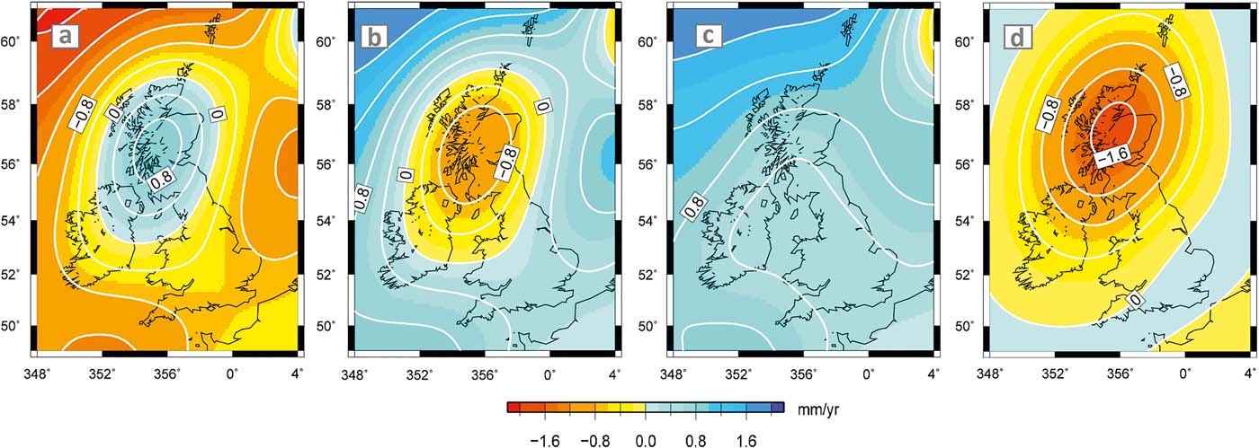
Figure 10 (a) Modelled present-day vertical land motion. (b) Modelled relative sea-level change. (c, d) Decomposed total sea-level signal from (b): (c) from far-field ice sheets; (d) from British–Irish ice sheet only. Copyright (2011) Wiley. Used with permission from Bradley, S. L., Milne, G. A., Shennan, I. & Edwards, R. J., An improved glacial isostatic adjustment model for the British Isles, Journal of Quaternary Science, John Wiley & Sons (License number 3758470726001).
3.3. Potential of SAR Interferometry for monitoring land uplift in northern Britain
Postglacial rebound has been investigated utilising a variety of measurement and modelling methods. Another powerful space geodesy tool for doing so might be found in synthetic aperture radar (SAR) interferometry. Differential SAR interferometry (DInSAR) is an established technique for analysing crustal motions and land deformations in terms of co-seismic processes, landslides or volcanic activity (e.g., Wright et al. Reference Wright, Lu and Wicks2003, Reference Wright, Parsons and Lu2004b; Pritchard et al. Reference Pritchard, Ji and Simons2006; Samsonov & d'Oreye Reference Samsonov and d'Oreye2012; Feng et al. Reference Feng, Li, Hoey, Zhang, Wang, Samsonov, Li and Xu2014; Singleton et al. Reference Singleton, Li, Hoey and Muller2014; Remy et al. Reference Remy, Chen, Froger, Bonvalot, Cordoba and Fustos2015). But it has also been widely used as a method for monitoring slower surface movements on a longer time scale, such as inter-seismic deformation or land subsidence due to groundwater and oil withdrawal or mining activities. It is also often combined with CGPS observations or levelling techniques as an independent data source (e.g., Hoffmann et al. Reference Hoffmann, Zebker, Galloway and Amelung2001; Tosi et al. Reference Tosi, Carbognin, Teatini, Strozzi and Wegmüller2002; Carbognin et al. Reference Carbognin, Teatini and Tosi2004; Wang et al. Reference Wang, Perissin, Liao and Rocca2008; Chen et al. Reference Chen, Liu, Ding, Hu, Yuan, Zhong and Omura2010; Fan et al. Reference Fan, Deng, Ju, Zhu and Xue2011; Osmanoğlu et al. Reference Osmanoğlu, Dixon, Wdowinski, Cabral-Cano and Jiang2011; Aobpaet et al. Reference Aobpaet, Cuenca, Hooper and Trisirisatayawong2013; Leighton et al. Reference Leighton, Sowter, Tragheim, Bingley and Teferle2013). DInSAR has proved useful for giving indirect information about GIA in areas where the ice sheet is still present. For example, it has been used in Antarctica to measure ice mass change and glacier flows and, thus, present clues about glacial rebound of the Antarctic continent (Sasgen et al. Reference Sasgen, Martinec and Bamber2010). However, research examining the applicability of DInSAR for monitoring wide-scale GIA land uplift directly, in any GIA affected region, is relatively scarce. Thus, the question for future research is what can be achieved at the direct interface between DInSAR and GIA (see Reference Bähr and HanssenFig. 11).
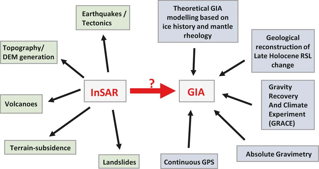
Figure 11 Interface between InSAR and GIA: research areas, where InSAR is commonly used as a tool (left) vs. research methods that are usually applied to analyse GIA (right). Research studying the application of InSAR to measure GIA-induced VLM directly has been scarce.
A review of DInSAR and land deformation monitoring is given by Massonnet & Feigl (Reference Massonnet and Feigl1998) and Crosetto et al. (Reference Crosetto, Crippa, Biescas, Monserrat, Agudo, Heipke, Jacobsen and Gerke2005). Recent advances using DInSAR time-series approaches for crustal deformation measurement are reviewed by Hooper et al. (Reference Hooper, Bekaert, Spaans and Arıkan2012). With conventional radar interferometry, two complex SAR images of the same area, acquired at the same time, but from different positions (measuring topography), or at different times (measuring deformation), are combined to generate an interferogram. For this, one acquisition is multiplied by the complex conjugate of another acquisition. See Hanssen (Reference Hanssen2001) for an in-depth description of the process. The phase of the interferogram is the phase difference between the two acquisitions, which is sensitive to surface height/topography and range changes in the line of sight of the radar. Conventional InSAR has been mostly used for generating topographic maps, prominently in the Shuttle Radar Topography Mission (SRTM). Temporal land surface changes are derived with differential interferometry, where usually a DEM is subtracted from the interferogram to eliminate the topographic phase from the total phase signal, in order to obtain the deformation phase component. An important prerequisite is that scattering properties on the ground stay the same, in order to create a high coherence between images and make the interferometric process possible. Usually, the longer the radar wavelength, the better a sensor is suited for the mitigation of such decorrelation effects. Data is available from several spaceborne SAR platforms, such as ESA's ERS-1/ERS-2, ESA's ENVISAT ASAR, ESA's recent Sentinel-1 mission, the Canadian Radarsat-1/-2, the Japanese ALOS PALSAR and ALOS-2 PALSAR-2, the Italian Cosmo-SkyMed and the German TerraSAR-X/TanDEM-X (see Reference BallantyneFig. 12). Together they contribute to an abundant global archive of SAR images for approximately the past 20 years, in different frequency bands of X-, C- and L-band and, thus, make it theoretically possible to observe GIA-related land uplift, for example, in Scotland.

Figure 12 Temporal coverage of available spaceborne SAR sensors and their frequency bands.
For the detection of long-term and very small, long-wavelength displacements, such as GIA, a very high quality standard in terms of precision and accuracy is necessary to make it a competitive tool to established geodetic techniques, such as CGPS (Crosetto et al. Reference Crosetto, Crippa, Biescas, Monserrat, Agudo, Heipke, Jacobsen and Gerke2005).
Under the right conditions, DInSAR can be sensitive to land deformations in the low-mm level (Crosetto et al. Reference Crosetto, Crippa, Biescas, Monserrat, Agudo, Heipke, Jacobsen and Gerke2005; Marinkovic et al. Reference Marinkovic, Ketelaar, van Leijen, Hanssen and Lacoste2008). The accuracy of DInSAR time-series techniques lies at 1 mm yr–1 for mean deformation velocity (Hammond et al. Reference Hammond, Blewitt, Li, Plag and Kreemer2012), but is dependent on weather conditions, the number of acquisitions available, the total time range covered by images and the distance to the reference area (Lanari et al. Reference Lanari, Casu, Manzo, Zeni, Berardino, Manunta and Pepe2007; Hooper et al. Reference Hooper, Bekaert, Spaans and Arıkan2012).
To achieve such precision and accuracy, conventional DInSAR techniques, where only two images are used, are insufficient. Over the last decade, methods for detecting long-term deformation have been improved by stacking several spaceborne SAR images of the same area, acquired through time. In this way, it is possible to describe the temporal evolution of deformations. Two prominent time-series techniques are known. The first one analyses the phase behaviour and scattering characteristics of a point scatterer in time and, thus, identifies pixels with minimal decorrelation noise (persistent scatterer) (Ferretti et al. Reference Ferretti, Prati and Rocca2001; Hooper et al. Reference Hooper, Zebker, Segall and Kampes2004; Costantini et al. Reference Costantini, Falco, Malvarosa and Minati2008). The second technique focuses on distributed scatterers and only uses interferograms between SAR images that are characterised by a small temporal and spatial baseline, so that decorrelation noise is minimised. An inversion of the interferograms then reveals the underlying cumulative deformation signal (small baseline subset InSAR or SBAS) (Berardino et al. Reference Berardino, Fornaro, Lanari and Sansosti2002; Lanari et al. Reference Lanari, Mora, Manunta, Mallorquí, Berardino and Sansosti2004, Reference Lanari, Casu, Manzo, Zeni, Berardino, Manunta and Pepe2007). In the case of high data redundancy, which means that several acquisitions are available for the observed area, a good precision and robustness can be achieved, addressing problems such as decorrelation and atmospheric and orbital effects (Crosetto et al. Reference Crosetto, Crippa, Biescas, Monserrat, Agudo, Heipke, Jacobsen and Gerke2005).
In general, the accuracy of the height change is only as good as the accuracy of the interferometric phase, which is influenced by several error sources. The total phase signal in an interferogram is usually a summation of several phase components:
 $$\phi_{total} = \phi_{deformation} + \phi_{orbit} + \phi_{atmosphere} + \phi_{topography} + \phi_{noise}$$
(Hanssen 2001), all of which have to be corrected for, when trying to extract the deformation signal φdeformation from φtotal.
A major limitation is finding areas with sufficient coherence of the ground targets. Temporal decorrelation, or phase noise (φnoise), is the most challenging problem with DInSAR, especially in terms of very slow land uplift (GIA) or subsidence. Very slow motion is more prone to temporal decorrelation, because it requires a longer observation period. This phenomenon can be addressed by bandpass filtering before interferogram generation, interferogram filtering or multi-looking (Hooper et al. Reference Hooper, Bekaert, Spaans and Arıkan2012). The permanent monitoring of slow deformation with CGPS has an advantage here, because it is not prone to such decorrelation effects. In addition, uncertainties in the DEM information that has been used for generating the differential interferogram cause topographic phase residuals (φtopography), which have to be considered and corrected (Ferretti et al. Reference Ferretti, Prati and Rocca2000; Crosetto et al. Reference Crosetto, Crippa, Biescas, Monserrat, Agudo, Heipke, Jacobsen and Gerke2005).
Additionally, the time-series techniques noted above address limits due to artefacts, superimposing signals due to atmospheric disturbances (φatmosphere) and uncertainties of satellite orbit parameters (φorbit). Those non-deformation artefacts can “swallow” the small motion process of GIA-induced uplift by introducing systematic errors in the DInSAR observations of displacements. Changes in atmospheric propagation between two acquisitions cause a signal delay and, thus, range differences. This atmospheric phase screen (APS) can become manifest in long radar wavelengths, such as L-band, caused by the ionosphere and, more commonly, across all radar frequencies due to tropospheric disturbances. The former is more of a problem in the case of long-wavelength deformation processes over hundreds of kilometres, while the latter presents a challenge for non-linear, non-steady deformations happening on a scale of tens of kilometres (Hooper et al. Reference Hooper, Bekaert, Spaans and Arıkan2012). In the case of a constant deformation rate, averaging/stacking several interferograms can decrease errors such as atmospheric effects (Hoffmann et al. Reference Hoffmann, Zebker, Galloway and Amelung2001; Wright et al. Reference Wright, Parsons and Fielding2001). However, estimating the non-deformation signal by modelling approaches is even better than averaging. Methods have been developed that use external information about atmospheric conditions (water vapour). The information may come from weather models, spectrometers, CGPS data about the tropospheric delay of a signal (Li et al. Reference Li, Muller, Cross and Fielding2005, Reference Li, Fielding, Cross and Muller2006, Reference Li, Fielding and Cross2009, Reference Li, Pasquali, Cantone, Singleton, Funning and Forrest2012), or relating topographic height with interferometric phase (Bekaert et al. Reference Bekaert, Hooper and Wright2015).
Orbital artefacts or phase ramps are especially problematic when it comes to measuring long-wavelength wide-scale ground deformation (GIA), since both often show similar spatial patterns, which are difficult to distinguish. Those errors are caused by inaccurate information about the orbit trajectories of the satellite at the times of acquisition. Algorithms for orbital error reduction take advantage of the fact that orbit errors are usually considered as uncorrelated over time, in contrast to deformation signals (Biggs et al. Reference Biggs, Wright, Lu and Parsons2007; Zhang et al. Reference Zhang, Ding, Lu, Jung, Hu and Feng2014). They simply fit either linear planes or two-dimensional polynomials empirically to the errors (Massonnet & Feigl Reference Massonnet and Feigl1998; Wright et al. Reference Wright, Parsons, England and Fielding2004a), and subtract them from the interferometric phase of an individual interferogram. Quadratic functions need to be applied with images covering more than 1000 km (Fournier et al. Reference Fournier, Pritchard and Finnegan2011). However, if the deformation signal shows similar characteristics, as is to be expected in the case of GIA land uplift in northern Britain, this would also eliminate the deformation signal from the interferograms. This means that more sophisticated methods are necessary, such as utilising networks of interferograms, rather than a single one, to fit planes to interferometric phases (Biggs et al. Reference Biggs, Wright, Lu and Parsons2007). Based on this network orbit correction technique, Feng (Reference Feng2014) and Stockamp et al. (Reference Stockamp, Li, Bishop, Hansom, Rennie, Petrie, Tanaka, Bingley, Hansen and Ouwehand2015) applied an extended method, which combines the conventional network approach with phase loop triplets of interferograms in order to introduce further observation equations that constrain parameters better. Another alternative is to use a network of interferograms for modifying orbit state vectors and estimating baseline errors directly (Bähr & Hanssen Reference Bähr, Hanssen and Lacoste-Francis2010, Reference Bähr and Hanssen2012). Furthermore, the separation of the long-wavelength deformation signal from orbital artefacts with GPS measurements is possible (e.g., Argus et al. Reference Argus, Heflin, Peltzer, Crampé and Webb2005; Pritchard et al. Reference Pritchard, Ji and Simons2006; Brooks et al. Reference Brooks, Merrifield, Foster, Werner, Gomez, Bevis and Gill2007; Lundgren et al. Reference Lundgren, Hetland, Liu and Fielding2009; Arıkan et al. Reference Arıkan, Hooper, Hanssen and Lacoste-Francis2010; Gourmelen et al. Reference Gourmelen, Amelung and Lanari2010; Wei et al. Reference Wei, Sandwell and Smith-Konter2010; Manzo et al. Reference Manzo, Fialko, Casu, Pepe and Lanari2012; Wang & Wright Reference Wang and Wright2012; Béjar-Pizarro et al. Reference Béjar-Pizarro, Socquet, Armijo, Carrizo, Genrich and Simons2013; Kaneko et al. Reference Kaneko, Fialko, Sandwell, Tong and Furuya2013; Tong et al. Reference Tong, Sandwell and Smith-Konter2013). The techniques to overcome problems in deformation extraction are continuously improved by the use of more frequent acquisitions, better elevation and atmospheric correction models and more sophisticated methods of precise orbit determination for better accuracy of satellite orbits.
Combination with another geodetic technique, such as CGPS, is also essential, when it comes to validation of the DInSAR results. In general, validation could be difficult with regard to the extension of the ground areas that are covered by DInSAR, when reference validation data are only sparse. The reference data must also be of equally high quality to that of the DInSAR data regarding precision and accuracy (Crosetto et al. Reference Crosetto, Crippa, Biescas, Monserrat, Agudo, Heipke, Jacobsen and Gerke2005).
The applicability and potential of DInSAR for determining vertical land motion (VLM) in the mm-level and in the context of relative sea-level change have been demonstrated, for instance, by Brooks et al. (Reference Brooks, Merrifield, Foster, Werner, Gomez, Bevis and Gill2007). They derived the VLM (induced by groundwater and oil extraction) at the coast of the Los Angeles basin between 1992 and 2000, with a persistent scatterer InSAR approach (C-band), tide gauge and CGPS observations. InSAR helped in determining the large spatial variability of VLM in that area, allowing the relative sea level in regions far away from tide gauge stations to be calculated along the coast with a high spatial resolution.
Persistent scatterer (PS) InSAR has also been successfully established on a regional level in Great Britain as a complementary technique to GPS and absolute gravity measurements for the monitoring of vertical land-level changes. Its applicability has been demonstrated in urbanised areas; for example, in the River Thames region (Bingley et al. Reference Bingley, Teferle, Orliac, Dodson, Williams, Blackman, Baker, Riedmann, Haynes, Aldiss, Burke, Chacksfield and Tragheim2007). Adamska (Reference Adamska2012) tested the suitability of using PS InSAR to measure regional VLM around selected tide gauges in the UK (Newlyn, Sheerness, Liverpool, North Shields), and to assess their stability, by referencing the relative InSAR measurements to absolute CGPS estimates. This author achieved good results for PS velocities despite unwanted influences by ocean tide loading on the deformation of the coastal areas.
For measuring more wide-spread glacial rebound in the UK, and especially in the central uplift regions of Scotland, the wide area coverage requires processing of bigger amounts of image data, although this could be limited by focusing on stable (exposed rocky) surfaces. SBAS could be more suitable than PS InSAR, due to the rural nature of most parts of the uplift area and the scarceness of dominant scatterers, such as man-made structures. This, however, also depends on the temporal sampling rate of acquisitions. In terms of addressing the issue of coherence in rural areas, the intermittent SBAS (ISBAS) (Sowter et al. Reference Sowter, Bateson, Strange, Ambrose and Syafiudin2013; Cigna et al. Reference Cigna, Rawlins, Jordan, Sowter and Evans2014b) approach, which includes intermittently or partially coherent areas, looks promising. The problem of temporal decorrelation might not be as much of a problem in northern Britain as it is in other GIA areas, such as Scandinavia or Canada. Due to its maritime climate, the snow cover period is shorter and less extensive in northern Britain. In addition, the land cover is more suitable for getting a good coherence for X- and C-band radar data, due to the lack of boreal forest or other forms of higher vegetation. This means that even shorter radar wavelengths (X- and C-band) might not be as affected by decorrelation (Rosen et al. Reference Rosen, Hensley, Zebker, Webb and Fielding1996).
In mountainous regions (highlands), DInSAR is seen as challenging. Liu et al. (Reference Liu, Shao, Liu, Riedel, Sowter, Niemeier and Bian2014), however, showed the application of SBAS for subsidence monitoring with L-, C- and X-band in a mountain area in China and produced promising results. In addition, a feasibility study undertaken by the British Geological Survey assessed the usability of PS InSAR to monitor ground motion on a nationwide scale in Great Britain, by investigating the use of appropriate SAR geometry of ERS-1/2 and ENVISAT to counteract geometric distortions, such as foreshortening, layover and shadowing, caused by local topography (Cigna et al. Reference Cigna, Bateson, Jordan and Dashwood2012, Reference Cigna, Bateson, Jordan and Dashwood2013, Reference Cigna, Bateson, Jordan and Dashwood2014a). Overall topographic visibility was determined to be good; i.e., active layover could only be found in a small proportion of Great Britain. Layover usually occurs at slopes facing the sensor, and when the slope angle is steeper than the SAR incidence angle. Then the upper part of the slope is seen as equally far away from the sensor as the lower slope part, and both areas appear at the same location in the SAR image, or are laid over each other. This can happen mostly in the very hilly regions of Scotland, and is dependent on the acquisition mode of ‘ascending’ or ‘descending’ and the orientation of the hill slopes towards the radar sensor's line of sight. No major shadow effects were discovered, due to the reasonably flat mountain slopes in Great Britain (Cigna et al. Reference Cigna, Bateson, Jordan and Dashwood2012).
To summarise, the continuous two-dimensional monitoring capabilities of DInSAR provide the advantage of measuring the GIA-induced vertical land motion directly over large areas (over 100 km-wide swaths), in contrast to techniques that focus on single point measurements and spatial interpolation. Many coherent points over the surface can be evaluated at relatively low effort and costs, and there is no ground measurement technique that could provide the same amount of sampling points. Thus, DInSAR could account better for the spatial variability of vertical land motion and its implications for relative sea-level trends, and it is not limited to the CGPS/AG/tide gauge network in Britain.
4. Conclusion
Several investigations that attempt to improve quantification and modelling of past and present glacial isostatic adjustment of the British Isles have been conducted in the last decades. This paper reviews some of those efforts with regard to the different observational data types, such as geological Late Devensian/ Holocene sea-level evidence and present-day geodetic information, which have been used for the constraint of GIA model parameters for the British Isles. An extensive data bank of sea-level index points from palaeo-environments around the British Isles has been built up that motivated the development of a variety of GIA models and helped in the derivation of long-term Holocene relative sea- and land-level estimates. Later studies examined the advantage of geodetic techniques, mainly CGPS, which help further parameterise the GIA models and give insight specifically into present-day vertical land motion. Despite this advance in GIA modelling for the British Isles, difficulties in parameterisation persist and poor fits between model and observations remain not uncommon, especially in Scotland. Different modelling approaches have tried to fit the same Holocene sea-level data, but significant differences regarding ice sheet history and Earth-model parameters remain in the modelling community. These misfits reflect the complex GIA situation of the British Isles, with a significant spatial and temporal variability in sea- and land-level change since the Last Glacial Maximum. The local isostatic component of the sea-level signal is of similar magnitude to that associated with the melt-water contribution from non-local ice sheets, but with opposite signs near the British ice sheet centre. Thus, strong non-monotonic sea-level changes were caused in time in the UK (Lambeck Reference Lambeck1993a, Reference Lambeckb; Milne et al. Reference Milne, Shennan, Youngs, Waugh, Teferle, Bingley, Bassett, Cuthbert-Brown and Bradley2006; Bradley et al. Reference Bradley, Milne, Teferle, Bingley and Orliac2009; Rennie & Hansom Reference Rennie and Hansom2011).
Maps of both the relative land-level change modelled with help of geological evidence (Shennan & Horton Reference Shennan and Horton2002; Shennan et al. Reference Shennan, Milne and Bradley2009) and the modelled vertical land motion constrained by data from geodetic techniques (Bradley et al. Reference Bradley, Milne, Teferle, Bingley and Orliac2009, Reference Bradley, Milne, Shennan and Edwards2011) show a similar pattern, with the centre of maximum uplift near the southwestern Grampian Highlands of Scotland, consistent with most CGPS maps. However, studies have also shown that geodetically derived estimates of vertical land motion can vary, depending on what CGPS processing strategy, time-series analysis approach and correction for temporal and spatial correlations has been used to derive the deformation velocities. In addition, the offset between CGPS and AG measurements in the vertical coordinate of ∼1mm yr–1, as reported by Teferle et al. (Reference Teferle, Bingley, Orliac, Williams, Woodworth, McLaughlin, Baker, Shennan, Milne and Bradley2009), cannot be ignored, considering the magnitude of the postglacial rebound signal is not much higher on the British Isles.
It is always important that results from the different geological and geodetic techniques are interpreted and compared with care, since they differ in applied processing and analysis methods, spatial sampling rates, time-scales, reference frames (relative land-/sea-level change or vertical land motion), and in the consideration of non-GIA related geophysical effects that influence crustal movements and sea levels.
Further research might give deeper insights into current rates of land uplift in northern Britain and its implications for relative sea-level change, by combining multiple satellite techniques, especially GNSS and SAR interferometry. Although notable challenges have to be expected when deriving very small, long-wavelength deformation signals from DInSAR data, techniques are in place to correct for these errors and limit uncertainties. The advantage of DInSAR is its high accuracy and spatial resolution, covering a wider area. It could close gaps in the quantitative description of the spatially diverse distribution of GIA, since the observational data density of conservative methods varies between regions. Geodetic methods provide information mostly limited to the existing CGPS/AG network, while Late Devensian/Holocene geological data are confined to accessible and preserved palaeo-environments. As another independent data source, DInSAR can help address biases in other geodetic techniques and vice-versa, thus demonstrating a complementary relationship between geodetic methods, as shown with CGPS and AG. Therefore, DInSAR might be beneficial in answering questions such as to what extent GIA-induced crustal uplift is still an issue at Scottish coasts today (Rennie & Hansom Reference Rennie and Hansom2011) and, thus, if a higher impact of rising sea levels at coasts is to be expected after all.
5. Acknowledgements
JS is supported by an EPSRC industry scholarship in association with Scottish Natural Heritage. The work is supported in part by the UK Natural Environment Research Council (NERC) through the LICS project (NE/K010794/1), the Key Laboratory of Earth Fissures Geological Disaster, Ministry of Land and Resources (Geological Survey of Jiangsu Province) through the KEYLAB/InSAR project, as well as the JAXA ALOS RA4 project (PI: 1358). We gratefully acknowledge the services of the Natural Environment Research Council (NERC) British Isles continuous GNSS Facility (BIGF), www.bigf.ac.uk, in providing archived GNSS data (and/or products) to this study. The authors thank David E. Smith and the anonymous referee for their valuable comments and their time spent on reviewing the manuscript.


