


1. Introduction
Although the linear dynamics solutions (e.g. Sverdrup gyres with Munk boundary layer approximation) produce some reasonable gyres, western boundary currents (WBCs) and planetary waves, they fail to simulate them correctly. Indeed, nonlinear circulation features, such as the eastward jet extension and its adjacent recirculation zones, are completely overlooked by the linear dynamics. The nonlinear dynamics solutions are capable of being realistic, provided that the mesoscales are adequately resolved. However, there are certain aspects of the wind-driven double-gyre circulation that still remain misunderstood. In this study, we work in the classical quasi-geostrophic (QG) double-gyre framework designed to mimic the wind-driven, midlatitude ocean circulation. The choice of this model results from its ability to resolve intricate nonlinear dynamics in long-time simulations.
The initial motivations of this study were the counter-rotating gyre anomalies (CGAs) (Shevchenko & Berloff Reference Shevchenko and Berloff2016), which are advection-induced, opposite-signed circulation anomalies embedded in the gyres. It was revealed, however, that not only the CGAs but also many other aspects of the double-gyre circulation are fundamentally controlled by non-trivial effects of flow nonlinearity near the western boundary. The remainder of this section discusses some of the important steps made in understanding the QG double-gyre circulation to help the reader contextualise the results made in this study.
1.1. Background
The impacts of nonlinear interactions on the background flow are vast and complex. Early studies with single- (Veronis Reference Veronis1966a,Reference Veronisb; Böning Reference Böning1986) and double-gyre (Holland Reference Holland1978; Haidvogel & Holland Reference Haidvogel and Holland1978; Holland & Rhines Reference Holland and Rhines1980) configurations used models with either lateral or bottom friction, or both. In the single-gyre case, an ocean gyre with a formation similar to an eastward jet occurred, often with a corresponding recirculation zone which increased the maximum mass transport (Böning Reference Böning1986). Veronis (Reference Veronis1966a,Reference Veronisb) found that effects of advection restructured the western boundary layer (WBL) by the cutting down of high velocities and vorticities. In the double-gyre case, symmetric wind forcing created two gyres of equal size separated by an eastward jet and recirculation zones. Mesoscale eddies were then generated by internal instabilities in the ocean currents which transferred energy from the upper to lower layers (Holland Reference Holland1978). Furthermore, theoretical discussions of eddy potential vorticity (PV) fluxes showed that within ‘special’ regions, such as eastward jet extensions, up-gradient movement of PV led to the induction of mean flow (Rhines & Holland Reference Rhines and Holland1979). Lozier & Riser (Reference Lozier and Riser1989) used a similar model to that used by Holland (Reference Holland1978), but with increased model resolution near the western wall. A Lagrangian particle analysis showed that fluid parcels passing through the viscous sublayer lost significantly less relative vorticity at the western boundary compared with the planetary vorticity gained. However, outside the viscous sublayer, but within the inertial boundary layer, fluid parcels lost an equal amount of relative vorticity as they gained planetary vorticity, thus, conserving PV. This indicated that the mechanisms acting within the viscous sublayer are different to those acting in the wider, inertial boundary layer.
A string of other studies that built upon this work were aimed at understanding how forcing asymmetries affect the double-gyre circulation. Harrison & Stalos (Reference Harrison and Stalos1982) introduced asymmetric wind forcing in a barotropic vorticity model with bottom friction. This led the eastward jet to disappear and instead be replaced with an overshooting subtropical WBC. Moro (Reference Moro1988, Reference Moro1990) then replaced bottom friction with lateral friction which created a meandering eastward jet with a vortex street pattern. Verron & Le Provost (Reference Verron and Le Provost1991) used a time-dependent multi-layer QG model, also with asymmetric wind forcing, and found a similar vortex street pattern in the eastward jet. Inter-gyre exchanges of PV through ring formations and vortex pinching were also found to be enhanced by the asymmetric wind forcing. Rhines & Schopp (Reference Rhines and Schopp1991) also parametrically adjusted the wind-curl asymmetry, which led to new branches of circulation being formed extending from the subtropical to subpolar gyre. A Lagrangian particle analysis also revealed that the mid-ocean showed dominant eddy mixing and that eddies were crucial in inter-gyre mixing. In fact, all of these phenomena were observed owing to the ocean gyres adjusting the large-scale circulation as a result of the vorticity imbalance created by asymmetric wind forcing. Haidvogel, McWilliams & Gent (Reference Haidvogel, McWilliams and Gent1992) implemented a partial-slip boundary condition parameter, which allowed for a continuous transition from the free-slip to no-slip flow regimes. It was found that varying this parameter had a basin-scale impact on both the time-mean circulation and eddy fields. In the free-slip limit, a flow regime similar to that of Holland (Reference Holland1978) was observed. However, transitioning to the no-slip limit led to a gradual retreat of the boundary current separation points until a double-jet structure was formed. Berloff & McWilliams (Reference Berloff and McWilliams1999a,Reference Berloff and McWilliamsb) explored different flow regimes with both free- and no-slip boundary conditions. The free-slip boundary condition was shown to have a stabilising effect on the WBCs, which extended into a single, narrow eastward jet. This behaviour was associated with enhanced large-scale low-frequency variability in the ocean gyres. Flow regimes with no-slip boundaries showed that the double-jet structure of Haidvogel et al. (Reference Haidvogel, McWilliams and Gent1992) was a robust phenomenon. Fox-Kemper (Reference Fox-Kemper2005) found that inter-gyre PV fluxes were inhibited by no-slip boundary conditions and only became important for free-slip boundary conditions. All these authors concluded that correct handling of boundary conditions is vital for correct simulation of the WBCs and large-scale circulation. Deremble et al. (Reference Deremble, Hogg, Berloff and Dewar2011) revisited the issue of lateral boundary conditions by applying the law of the wall theory, which has had success in atmospheric boundary layer dynamics (Fairall et al. Reference Fairall, Bradley, Hare, Grachev and Edson2003). It was found that applying such boundary conditions resembled flow regimes under free-slip boundary conditions rather than no-slip. It was concluded that a partial-slip boundary condition parameter, chosen close to the free-slip limit, was most suitable as it also allowed momentum and vorticity flux through the boundaries.
Another important aspect of the ocean gyres are the recirculation zones that lie on either side of eastward jet extensions. Cessi, Ierley & Young (Reference Cessi, Ierley and Young1987) noted that the recirculation zones are driven by anomalous values of PV carried through the WBCs; Jayne, Hogg & Malanotte-Rizzoli (Reference Jayne, Hogg and Malanotte-Rizzoli1996) showed eddies acted to smooth out extrema to create uniform plateaus of PV. Kiss (Reference Kiss2002) also found that a non-turbulent, unstratified model with lateral friction generated high values of PV within the WBCs owing to an insufficient loss of PV in the viscous sublayer, similar to the results obtained by Cessi et al. (Reference Cessi, Ierley and Young1987) and Lozier & Riser (Reference Lozier and Riser1989). These results were extended to a stratified, turbulent model by Kiss (Reference Kiss2010), where PV fluxes replaced eddy viscosity as the dominant mechanism in generating anomalous PV. A study using Lagrangian particle analysis (Ypma et al. Reference Ypma, van Sebille, Kiss and Spence2016) was also found to be consistent with their results using an ocean general circulation model. Nakano, Tsujino & Furue (Reference Nakano, Tsujino and Furue2008) went further to classify the PV sources feeding the recirculation zones into three types: inertial, directly forced and instability forced. These recirculation zones then drive the eddy backscatter mechanism (e.g. Berloff Reference Berloff2005, Reference Berloff2016; Shevchenko & Berloff Reference Shevchenko and Berloff2016), which acts to fortify the eastward jet.
Inter-gyre PV fluxes have been shown to modulate the transition between key states of low-frequency modes (Berloff, Hogg & Dewar Reference Berloff, Hogg and Dewar2007b) despite the eastward jet acting as a partial inter-gyre barrier for fluid parcels (Berloff, McWilliams & Bracco Reference Berloff, McWilliams and Bracco2002). Such low-frequency modes are important owing to their potential to project variability upon existing modes in the atmosphere by modifying their time scales (Hogg et al. Reference Hogg, Dewar, Killworth and Blundell2006; Berloff et al. Reference Berloff, Dewar, Kravtsov and McWilliams2007a). More recently, nonlinear circulation features known as CGAs, which consist of circulation anomalies embedded in the WBL and ocean interior, have been found (Shevchenko & Berloff Reference Shevchenko and Berloff2016). The CGAs weaken the double-gyre circulation and work against eddy backscatter, thus, suggesting a potential influence of the WBLs on the large-scale circulation through inter-gyre PV fluxes (Shevchenko & Berloff Reference Shevchenko and Berloff2016). Indeed, a link between insufficient loss of PV in the viscous sublayers (e.g. Lozier & Riser Reference Lozier and Riser1989) and inter-gyre PV fluxes has yet to be made.
In § 2, we describe the ocean model and methods for analyses of reference solutions. A detailed analysis of the ocean gyres, including the CGAs, is covered in § 3. We also make hypotheses upon the control of the WBLs on the ocean gyres and the nature of the inter-gyre PV exchange. Finally, a Lagrangian particle analysis is performed in § 4 to confirm the existence of the inter-gyre PV exchange and support hypotheses made in § 3. Results of the study and potential further aspects of research are discussed in § 5.
2. Ocean model and methods
The following section provides a background of the model and methods used in this study. Reference solutions are also provided within this section.
2.1. Quasi-geostrophic equations
The ocean model we used was identical to that used by Berloff (Reference Berloff2015). We considered an idealised, eddy-resolving QG model with three stacked isopycnal layers. It was designed to mimic the wind-driven, midlatitude, double-gyre ocean circulation. The ocean basin was configured as a flat-bottomed square box with  $(x,y)$ as zonal and meridional coordinates. The square basin
  $D(x,y)$ had length
  $2L=3840\ \textrm {km}$ and depths
  $H_k=250\ \textrm {m}$,
  $750\ \textrm {m}$,
  $3000\ \textrm {m}$ for
  $k=1,2,3$ with
  $-L\leqslant x\leqslant L$ and
  $-L\leqslant y \leqslant L$. The governing QG equations are given in terms of the streamfunction
  $\psi _i$ and PV anomalies
  $q_i$, which are defined by
 $$\begin{gather} q_1=\nabla^2\psi_1-S_{11}(\psi_1-\psi_2), \end{gather}$$
 $$\begin{gather}q_2=\nabla^2\psi_2-S_{21}(\psi_2-\psi_1)-S_{22}(\psi_2-\psi_3), \end{gather}$$
 $$\begin{gather}q_3=\nabla^2\psi_3-S_{31}(\psi_3-\psi_2) , \end{gather}$$
where the stratification parameters  $S_1, S_{21}, S_{22}, S_3$ are defined by the first and second baroclinic Rossby deformation radii, chosen to be
  $40.0\ \textrm {km}$ and
  $20.6\ \textrm {km}$, respectively. This then allows us to formulate the QG equations:
 $$\begin{gather} \frac{\partial q_1}{\partial t}+J(\psi_1,q_1)+\beta \frac{\partial \psi_1}{\partial x}=\frac{1}{\rho_1 H_1}W+\nu \nabla^4\psi_1 , \end{gather}$$
 $$\begin{gather}\frac{\partial q_2}{\partial t}+J(\psi_2,q_2)+\beta \frac{\partial \psi_2}{\partial x}=\nu \nabla^4\psi_2 , \end{gather}$$
 $$\begin{gather}\frac{\partial q_3}{\partial t}+J(\psi_3,q_3)+\beta \frac{\partial \psi_3}{\partial x}={-}\gamma\nabla^2\psi_3+\nu \nabla^4\psi_3 , \end{gather}$$
where  $\beta =2\times 10^{-11}\ \textrm {m}^{-1}\ \textrm {s}^{-1}$ is the planetary vorticity gradient,
  $\rho _1=1000\ \textrm {kg}\ \textrm {m}^{-3}$ is the upper-layer density,
  $\nu =20\ \textrm {m}^2\ \textrm {s}^{-1}$ is the eddy viscosity coefficient,
  $\gamma =4\times 10^{-8}\ \textrm {s}^{-1}$ is the bottom friction parameter and
  $J(\cdot ,\cdot )$ is the Jacobian operator.
The asymmetric wind forcing was fixed in time and defined as
 \begin{equation} W(x,y) =
\left\{\begin{array}{@{}ll}
-\dfrac{{\rm \pi}\tau_0A}{2L}\sin\left[\dfrac{{\rm \pi}(L+y)}{L+Bx}\right],
& \textrm{if }y\leqslant Bx, \\
+\dfrac{{\rm \pi}\tau_0}{2LA}\sin\left[\dfrac{{\rm \pi}(y-Bx)}{L-Bx}\right],
& \textrm{if }y> Bx. \end{array} \right.
\end{equation}
\begin{equation} W(x,y) =
\left\{\begin{array}{@{}ll}
-\dfrac{{\rm \pi}\tau_0A}{2L}\sin\left[\dfrac{{\rm \pi}(L+y)}{L+Bx}\right],
& \textrm{if }y\leqslant Bx, \\
+\dfrac{{\rm \pi}\tau_0}{2LA}\sin\left[\dfrac{{\rm \pi}(y-Bx)}{L-Bx}\right],
& \textrm{if }y> Bx. \end{array} \right.
\end{equation}
where  $A=0.9$,
  $B=0.2$ and
  $\tau _0=0.08\ \textrm {Nm}^{-2}$. The extra factor of
  $1/2$ in (2.3) and an order of magnitude correction in
  $\tau$ are both rectifications of typos by Berloff (Reference Berloff2015). Note that
  $A$ and
  $B$ are parameters that control the degree of asymmetry in the wind forcing. Partial-slip boundary conditions
  $\psi _{\boldsymbol {nn}}=\alpha \psi _{\boldsymbol {n}}$, where
  $\boldsymbol {n}$ is the normal-to-wall unit vector, were enforced on the lateral boundaries (Haidvogel et al. Reference Haidvogel, McWilliams and Gent1992). Mass conservation constraints were applied for each layer (McWilliams Reference McWilliams1977). The partial-slip boundary condition parameter
  $\alpha =120\ \textrm {km}$ was chosen such that it was close to a free-slip boundary condition but still allowed for momentum flux through the lateral boundaries (Deremble et al. Reference Deremble, Hogg, Berloff and Dewar2011). The equations were solved using the CABARET scheme (Karabasov, Berloff & Goloviznin Reference Karabasov, Berloff and Goloviznin2009) with a nominal resolution of
  $7.5\ \textrm {km}$, which corresponded to a uniform
  $513^2$ grid. The model was integrated for 60 model years with a 20-year spin-up period. Data were accumulated every model day.
We present typical snapshots and time-mean solutions of system (2.2) in figures 1 and 2, respectively. Wind acting on the upper isopycnal layer created the double-gyre flow regime through the imposed large-scale Ekman pumping anomalies. The two gyres were separated by the powerful eastward jet, which was supported by the subpolar and subtropical WBCs. Strong eddy activity was visible in the upper isopycnal layer around the WBC separation point and eastward jet, while the lower layers were dominated by weaker eddies. The middle isopycnal layer also showed a region of uniform PV, which was homogenised by eddies (Rhines & Young Reference Rhines and Young1982; Lozier & Riser Reference Lozier and Riser1989).

Figure 1. Instantaneous snapshots of the statistically equilibrated reference solution of system (2.2). (a–c) Velocity streamfunctions in the upper, middle and lower isopycnal layers, respectively. (d–f) PV anomalies in the upper, middle and lower isopycnal layers, respectively. For presentation purposes, the colour-bar range for each plot is determined by the maximum and minimum values. This is repeated for all consequent plots unless stated otherwise. Values of Max for each panel are stated for comparison. (a)  $\textrm {Max} = 7.3\times 10^4\ \textrm {m}^2\ \textrm {s}^{-1}$. (b)
  $\textrm {Max} = 3.3\times 10^4\ \textrm {m}^2\ \textrm {s}^{-1}$. (c)
  $\textrm {Max} = 2.4\times 10^4\ \textrm {m}^2\ \textrm {s}^{-1}$. (d)
  $\textrm {Max} = 1.1\times 10^{-4}\ \textrm {s}^{-1}$. (e)
  $\textrm {Max} = 2.5\times 10^{-5}\ \textrm {s}^{-1}$. (f)
  $\textrm {Max} = 1.5\times 10^{-5}\ \textrm {s}^{-1}$.

Figure 2. Time-mean solutions of system (2.2) in statistical equilibrium. (a–c) Velocity streamfunctions in the upper, middle and lower isopycnal layers, respectively. (d–f) PV anomalies in the upper, middle and lower isopycnal layers, respectively. Inter-gyre boundary, shown in (a), is defined by the time-mean contour emanating from the western boundary. Values of Max for each panel are stated for comparison. (a)  $\textrm {Max} = 6.0\times 10^4\ \textrm {m}^2\ \textrm {s}^{-1}$. (b)
  $\textrm {Max} = 2.3\times 10^4\ \textrm {m}^2\ \textrm {s}^{-1}$. (c)
  $\textrm {Max} = 9.7\times 10^3\ \textrm {m}^2\ \textrm {s}^{-1}$. (d)
  $\textrm {Max} = 7.1\times 10^{-5}\ \textrm {s}^{-1}$. (e)
  $\textrm {Max} = 1.7\times 10^{-5}\ \textrm {s}^{-1}$. (f)
  $\textrm {Max} = 5.5\times 10^{-6}\ \textrm {s}^{-1}$.
2.2. Linearised dynamics
As we were interested in studying advection-induced anomalies, we also required solutions for the linearised dynamics. System (2.2) was linearised around the state of rest to give
 $$\begin{gather} \frac{\partial q_1}{\partial t}+\beta \frac{\partial \psi_1}{\partial x}=\frac{1}{\rho_1 H_1}W+\nu \nabla^4\psi_1 , \end{gather}$$
 $$\begin{gather}\frac{\partial q_2}{\partial t}+\beta \frac{\partial \psi_2}{\partial x}=\nu \nabla^4\psi_2 , \end{gather}$$
 $$\begin{gather}\frac{\partial q_3}{\partial t}+\beta \frac{\partial \psi_3}{\partial x}={-}\gamma\nabla^2\psi_3+\nu \nabla^4\psi_3 . \end{gather}$$
The parameters for these equations, as well as the configuration of the numerical CABARET solver, were identical to system (2.2). These equations are also studied analytically in Appendix A by generalising the Munk boundary layer solution (Munk Reference Munk1949) for partial-slip boundary conditions.
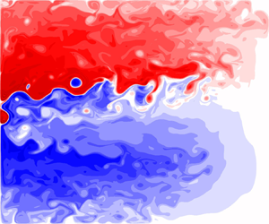
Figure 3 shows that the Sverdrup (i.e. linear) gyres and WBCs in the upper isopycnal layer were present but differed from the nonlinear dynamics solutions. Furthermore, nonlinear phenomena, such as the eastward jet and recirculation zones, were missing. Contours plots for the lower layers were omitted as these only show the gravest basin modes propagating across the basin. This is because the eddy forcing that drives the lower layers (Holland Reference Holland1978) was no longer present.

Figure 3. Contour plots of time-mean solutions for system (2.4) in the upper isopycnal layer. Values of Max for each panel are stated for comparison. (a) Velocity streamfunction,  $\textrm {Max} = 7.0\times 10^4\ \textrm {m}^2\ \textrm {s}^{-1}$. (b) PV anomaly,
  $\textrm {Max} = 3.7\times 10^{-4}\ \textrm {s}^{-1}$. Inter-gyre boundary in (a) is defined in the same manner as discussed in the caption of figure 2.
2.3. Lagrangian particles
In the subsequent sections, we use a Lagrangian particle analysis to identify inter-gyre particle pathways. Such techniques are useful owing to their ability to capture ensemble behaviour of fluid parcels, and hence, long-range material transports. For example, through the Lagrangian framework, we are able to study the long-range transport of PV, to which the Eulerian framework is not well suited.
Simulations were run by releasing an ensemble of  $N$ particles into the upper isopycnal layer and solving
 \begin{equation} \frac{\textrm{d}\boldsymbol{x}_j(t)}{\textrm{d}t}=\boldsymbol{u}(t,\boldsymbol{x}_j(t)),\quad \textrm{for } j=1,\ldots,N , \end{equation}
where  $\boldsymbol {x}_j(t)$ is the position of particle
  $j$ at time
  $t$ and
  $\boldsymbol {u}(t,\boldsymbol {x})=(u(t,\boldsymbol {x}), v(t,\boldsymbol {x}))$ is the velocity of the flow at position
  $\boldsymbol {x}$ and time
  $t$. System (2.5) was solved offline using the 4th-order Runga–Kutta scheme with a two-dimensional (2-D) cubic spatial interpolation and a one-dimensional (1-D) cubic temporal interpolation. Total PV
  $(Q=q+\beta y)$ was estimated along the trajectories by using a 2-D cubic interpolation (Total PV was used for Lagrangian particle analysis rather than PV anomalies because it is a materially-conserved quantity.).
3. Influences of nonlinearity on the ocean gyres
3.1. Nonlinear western boundary layer
The differences in structure of the upper-layer WBL were particularly significant when inspecting figures 2 and 3. Figure 3(b) shows much stronger zonal PV gradients near the western boundary, which are accompanied by increased meridional velocities in the region. Typical time-mean meridional velocities for system (2.2) were  $1\ \textrm {ms}^{-1}$, while they were up to
  $4\ \textrm {ms}^{-1}$ for system (2.4). This implied a cutting down of the high velocity and vorticity in the WBL through nonlinear effects. Indeed, Veronis (Reference Veronis1966a) also showed through a perturbation analysis that this restructuring of the WBL is likely owing to the meridional inhomogeneities in the structure of the wind forcing and ocean gyres. Furthermore, they showed that this restructuring is controlled by effects of PV advection. However, it is unclear what processes maintain the structure of the WBL after the assumptions of the stability analysis break down. A full analysis of the advection term in (2.2a) is required to understand this, which is outside the scope of this study. Reduction of WBC velocities also indicates that the nonlinear dynamics solutions will also show a reduction in viscous relative vorticity fluxes through the western boundary in comparison to the linear dynamics solutions (Spall Reference Spall2014, see also § 3.3). We now continue our analysis by defining the CGAs through a solution decomposition.
3.2. Solution decomposition
The CGAs, as well as other nonlinear circulation features, are defined by decomposing the nonlinear dynamics solutions into the linear dynamics (subscript ‘lin’), time-mean advection-induced nonlinear anomalies (subscript  $\oplus$) and transient fluctuations (primed):
 \begin{equation} \psi_i = \bar{\psi}_{i,{lin}} + \bar{\psi}_{i,\oplus} + \psi_i' , \end{equation}
for layers  $i=1,2,3$ (see Shevchenko & Berloff (Reference Shevchenko and Berloff2016) for identical decomposition). Note that the time-mean streamfunction is given by
  $\bar {\psi }_i=\bar {\psi }_{i,{lin}} + \bar {\psi }_{i,\oplus }$. This process was also repeated for PV anomalies. We chose this particular decomposition as we wanted to highlight the regions where the discrepancy between the nonlinear dynamics solutions, i.e. system (2.2), and linear dynamics solutions, i.e. system (2.4), was the greatest. This then allowed us to pinpoint the regions where nonlinear effects were particularly strong, which will guide our analysis in later sections. Comparisons of the nonlinear dynamics against the linear dynamics have been used in the past to study recirculation zones and eastward jets (e.g. Veronis Reference Veronis1966a; Harrison & Stalos Reference Harrison and Stalos1982), and we will be using the same technique for the CGAs.
The time-mean advection-induced anomalies (figure 4) revealed the recirculation zones on either side of the eastward jet, and the sharp zonal PV anomaly gradients near the western boundary that extended out into the gyre interiors. The CGAs were seen to be embedded in the subpolar (subtropical) gyres as opposite-signed, anti-cyclonic (cyclonic) anomalies. We stress here that because the CGAs were defined as a deviation from the linear dynamics solutions, they would not necessarily be visible in observations/models without this particular solution decomposition. However, because the decomposition was available to us, we will show that these anomalies are dynamically important and linked to mechanisms that control the double-gyre circulation.

Figure 4. Contour plots of time-mean advection-induced anomalies in the upper isopycnal layer for the reference, statistically equilibrated flow regime. Values of Max for each panel are stated for comparison. (a) Velocity streamfunction,  $\textrm {Max}=6.0\times 10^4\ \textrm {m}^2\ \textrm {s}^{-1}$. (b) PV anomaly,
  $\textrm {Max}/5=6.5\times 10^{-5}\ \textrm {s}^{-1}$. See figure 5 for zoomed-in plots of PV anomalies near the western boundary. Use of colour-bar range for (a) is the same as that in figure 1, but the colour-bar range for (b) is limited to 1/5 of the maximum value to better show the anomalies in the ocean interior, as they are weak compared with the anomalies in the WBL. Box surrounded by black dotted lines indicates the region near the western boundary plotted in figure 5.
Upon further inspection of these anomalies, we see that they were, in fact, two separate lobes (see figure 5c). The first lobe, which was by far the stronger anomaly, was situated within the viscous sublayer of the WBLs. We will refer to this lobe as the ‘WBL lobe’ for brevity. The second lobe, which was a much weaker but larger anomaly, was spread throughout the western half of each gyre interior. This lobe will be referred to as the ‘interior lobe’. Why the CGAs were separated into two separate lobes and the influences of nonlinearity in this regions on the global circulation is still not fully known.

Figure 5. Contour plots of time-mean PV anomalies in the upper isopycnal layer near the western boundary. Figures are zoomed-in to show the region outlined in figure 4. Values of Max for each panel are stated for comparison. (a) Nonlinear dynamics solution,  $\textrm {Max} = 7.1\times 10^{-5}\ \textrm {s}^{-1}$. (b) Linear dynamics solution,
  $\textrm {Max} = 3.7\times 10^{-4}\ \textrm {s}^{-1}$. (c) Time-mean advection-induced anomalies,
  $\textrm {Max} = 3.2\times 10^{-4}\ \textrm {s}^{-1}$. Areas that contain the subtropical WBL and interior lobes of the CGAs are marked by dotted lines in (c). Note that the interior lobe extends further outside of (c) into the ocean interior.
For the lower layers, the equivalent plots for figure 4 are shown in figure 2(b,c,e,f). This is because the lower layers were essentially stagnant for the linear dynamics solutions. Inspecting these plots, we observed that the recirculation zones were visible in the lower layers but no CGA-like patterns were present. Thus, we concluded that the CGAs were confined to the upper isopycnal layer, which was the only layer driven directly by wind-stress curl. This indicated that wind-stresses are important in the emergence of the CGAs.
Shevchenko & Berloff (Reference Shevchenko and Berloff2016) found that by strengthening the CGAs through an external forcing term, the eastward jet was weakened. However, they did not analyse in detail the dynamics associated with them. We continue our analysis of the CGAs by examining the relative-vorticity fluxes at the western boundary, where the time-mean advection-induced anomalies are strongest.
3.3. Excess PV buildup
To better understand how nonlinear effects adjust the large-scale circulation in the upper isopycnal layer, we calculated the PV budgets for both the linear and nonlinear dynamics solutions. A similar budget was computed by Berloff et al. (Reference Berloff, Hogg and Dewar2007b), albeit with different model configurations. The sources and sinks of PV in the upper isopycnal layer are considered below and PV fluxes are estimated and given in table 1.
Table 1. PV budgets for linear and nonlinear dynamics solutions for the subtropical gyre in the upper isopycnal layer. PV sources are estimated using time-mean values with units  $\textrm {m}^2\ \textrm {s}^{-2}$. Bracketed values are identical computations made for the subpolar gyre. Terms that account for
  ${<}0.05\,\%$ of the budget are deemed as negligible. We find that the PV budget is largely insensitive to small changes made in the inter-gyre boundary.

To compute a PV budget for each gyre, we need an inter-gyre boundary. This was calculated by following the time-mean contour emanating from the western boundary, which extended eastward across the basin. In the linear dynamics solutions, the inter-gyre boundary was a straight line dividing the two gyres (figure 3a). However, in the nonlinear dynamics solutions, the inter-gyre boundary was given by the time-mean eastward jet position (figure 2a). Note that the time-mean contour was particularly difficult to compute near the eastern boundary, where the eastward jet extension tore itself apart. However, we found that small changes to this inter-gyre boundary had negligible effects on the results from the subsequent PV budget.
The only source of PV for the gyres was through Ekman pumping anomalies generated by wind-curl. This was calculated by integrating (2.3) over each gyre:
 \begin{equation} G_W = \int_{{gyre}} W(x,y)\,\textrm{d} x\,\textrm{d} y . \end{equation}
We note here a phenomenon, which was more pronounced in the nonlinear dynamics solutions, and is referred to as the geometric wind effect (Berloff et al. Reference Berloff, Hogg and Dewar2007b). When the eastward jet extension was situated north of the zero wind-curl line, this led to a  ${\sim }10\,\%$ attenuation of the wind-curl input for both gyres (table 1). A similar but weak effect occurred in the linear dynamics solutions, as the zero wind-curl line is given by the line of zero meridional velocity instead of zero total velocity (Rhines & Schopp Reference Rhines and Schopp1991). However, this only had a small effect on the wind-curl inputs for each gyre (
 ${<}1\,\%$), so we neglected this effect on the linear dynamics.
The sink terms of the PV budget were computed by considering the viscous boundary and inter-gyre PV fluxes. Viscous boundary fluxes were calculated as
 \begin{equation} G_{VB} = \nu\overline{\int_{C\backslash\varGamma}\boldsymbol{\nabla}\left(\nabla^2\psi\right) \boldsymbol{\cdot}\boldsymbol{n}\,\mathrm{d}s}, \end{equation}
where  $\boldsymbol {n}$ is the corresponding outward normal,
  $C$ is the contour running along the exterior of the gyre and
  $\varGamma$ is the inter-gyre boundary. The overline denotes the time averaging over the reference solution.
The inter-gyre viscous fluxes were negligible in the linear dynamics, where they accounted for  ${<}0.05\,\%$ of the budget. They also remained extremely small in the nonlinear dynamics solutions, but we included them to close the PV budget. They were computed similarly to (3.3), as
 \begin{equation} G_{IV} = \nu\overline{\int_{\varGamma}\boldsymbol{\nabla}\left(\nabla^2\psi\right) \boldsymbol{\cdot}\boldsymbol{n}\,\mathrm{d}s} , \end{equation}
except that we integrated over the inter-gyre boundary, rather than along the basin boundary.
The inter-gyre PV fluxes were computed by projecting the PV anomaly fluxes onto unit normal vectors of the inter-gyre boundary:
 \begin{equation} G_{IF} ={-}\overline{\int_{\varGamma} q\boldsymbol{u}\boldsymbol{\cdot}\boldsymbol{n}\,\mathrm{d}s} . \end{equation}
A proportion of this will consist of inter-gyre exchanges of PV through the action of mesoscale eddies, while the remainder consists of contributions arising from the time-mean flow. Note that PV fluxes owing to the time-mean flow were non-zero because the eastward jet extension did not reach the eastern boundary. The inter-gyre eddy PV fluxes largely presided over the eastward jet, where there was zero time-mean flow across it; while the inter-gyre time-mean PV fluxes occurred further east, where there was a ‘gap’ between the eastward jet and eastern boundary for flow to pass through.
Finally, we must consider the tendency term as, owing to the decadal variability of the ocean gyres in the nonlinear dynamics solutions, its time average is non-zero:
 \begin{equation} G_T ={-}\overline{\int_{{gyre}}\frac{\partial q}{\partial t}\,\textrm{d} x\,\textrm{d} y} . \end{equation}
Overall, we must have PV anomaly conserved over each gyre, i.e.
 \begin{equation} G_W+G_{VB}+G_{IV}+G_{IF}+G_T = 0 , \end{equation}
the results of which are shown in table 1. Note that the  $\beta$-term contributions to the budget were zero through mass conservation.
Because the WBL lobes of the CGAs consisted of strong negative (positive) advection-induced PV anomalies in the subpolar (subtropical) WBL, we expected a reduction in the zonal relative vorticity gradients near the western boundary, which is confirmed in figure 6. Indeed, this led to  ${>}80\,\%$ reduction in viscous boundary fluxes (table 1), which was balanced by the inter-gyre PV fluxes. The sign change in advection-induced PV anomalies at the western boundary did not increase the magnitude of relative vorticity in this region, but instead reduced it, as there was also a corresponding sign change in the relative vorticity near the western boundary. This then led to a reduction in viscous boundary fluxes, as they are governed by normal derivatives of the relative vorticity.

Figure 6. Time-mean relative vorticity profiles near the western boundary of linear and nonlinear dynamics solutions, and advection-induced anomalies. The generalised Munk boundary layer solution (see Appendix A) is added to compare with the linear dynamics solution. Profiles have been meridionally averaged over (a) subtropical gyre, (b) subpolar gyre.
These results were consistent with those made by Cessi et al. (Reference Cessi, Ierley and Young1987) and Kiss (Reference Kiss2002), where there was also insufficient loss of PV. Cessi et al. (Reference Cessi, Ierley and Young1987) showed that the excess PV then drives the recirculation zones, and Kiss (Reference Kiss2002) argued that this effect may also be involved in the WBC separation. Our results differed from these studies, as we used a double-gyre, rather than a single-gyre model. This gave the model an extra mechanism to remove excess PV, which was through the inter-gyre PV fluxes downstream of the WBCs.
The extent to which the CGAs were consistent with a linear response to the geometric wind effect was checked by reducing the wind-stress amplitude  $\tau _0$ by 20 % (We define the linear response to the geometric wind effect as the difference between the time-mean linear dynamics solutions for 80 % and 100 % wind-stress amplitudes.). This was to mimic the impact of the geometric wind effect on wind-curl input reduction for each gyre. We will see from the results of this experiment that even by overestimating the impact of the geometric wind effect, the linear response alone was not strong enough. Relative vorticities, rather than PV anomalies, were used to show the linear response, as they determine the viscous boundary fluxes. Figure 7(a) shows anti-cyclonic (cyclonic) anomalies situated within the subpolar (subtropical) WBL, similar to the WBL lobe of the CGAs seen in figure 5(c). Furthermore, figure 7(b) shows a weaker, second lobe similar to those observed in figure 4(b). However, the linear response to reduced wind-curl input in the ocean interior was basin-wide, rather than being confined to the western half of the gyres. This implied that the shape of the CGAs was consistent with a linear response to the geometric wind effect but this alone could not account for the nonlinear dynamics anomalies, which were significantly stronger. Indeed, the linear response only accounted for
  ${\sim }15$% of the viscous boundary flux reduction drop, which may also be seen by comparing the PV budgets of the linear and nonlinear dynamics solutions (table 1).

Figure 7. Contour plots of the time-mean, linear, weakened wind-curl response for relative vorticities in the upper isopycnal layer. Values of Max for each panel are stated for comparison (e.g. with figure 5c). (a) Zoomed-in WBL region,  $\textrm {Max} = 8.5\times 10^{-5}\ \textrm {s}^{-1}$. (b) Ocean interior,
  $\textrm {Max}=1.9\times 10^{-7}\ \textrm {s}^{-1}$.
The separation of the two lobes of the CGAs (figure 5) also suggested that the mechanisms that drive these circulation features were unlikely to be the same. To confirm this, we produced scatter plots of PV anomalies against the velocity streamfunction (see figure 8). In the interior lobe, we observed a functional (nearly linear) relationship between PV anomaly and velocity streamfunction values, which implied the formation of Fofonoff-type gyres (Fofonoff Reference Fofonoff1954). However, in the WBL, the effects of friction made the above-mentioned relationship unfeasible.

Figure 8. Scatter plots of PV anomalies against velocity streamfunction for grid points in the interior and WBL lobes of the CGAs: (a) subtropical gyre, (b) subpolar gyre.
Examining the inter-gyre PV fluxes in table 1, we see they took up a considerably larger proportion of the PV budget compared with that reported by Berloff et al. (Reference Berloff, Hogg and Dewar2007b). This was attributed to the much smaller eddy-viscosity parameter and a boundary condition parameter choice which created a more turbulent flow regime. Because higher inter-gyre PV fluxes were directly associated with stronger advection-induced anomalies in the WBL, we expected CGAs to only become observable in more nonlinear flow regimes. Along with the drop in viscous boundary fluxes, the inter-gyre PV flux increase accounted for the largest changes in the PV budget for the linear and nonlinear dynamics solutions.
To understand the chain of events that led to both the viscous boundary flux reduction and increase in inter-gyre PV fluxes, we performed a numerical experiment, where we solved system (2.2), but used the time-mean solution to system (2.4) as the initial condition. What we would expect to see is the time-mean linear dynamics solution (figure 3) to converge towards the nonlinear dynamics solutions (figure 2), thus, leading to the adjustments in the PV budgets observed in table 1. The time scales associated with these adjustments can help us to identify the likely causal chains taking place. For example, it may be the case that viscous boundary flux reductions, induced by the nonlinear boundary layer, create a PV accumulation which must be rectified by the inter-gyre PV fluxes. Then, we would expect the time scale of this PV budget adjustment in our experiment to be of WBC advective time scales  $T_{{wbc}} \sim L/U\approx 11\ \textrm {days}$, where
  $L$ is the basin length scale and
  $U=2\ \textrm {ms}^{-1}$ is the WBC velocity scale. Alternatively, the uptake in inter-gyre PV fluxes could reduce PV concentrations within each gyre, which then reduce the viscous boundary fluxes. If this were the case, then we would expect to see the PV budget adjustment to take place over gyre recirculation time scales
  $T_{{gyre}}\approx {O}(1\ \textrm {year})$. We found that the viscous boundary flux adjustment took place over an extremely short time frame
  $({\sim }20\ \textrm {days})$, which indicated that it is the WBC advective time scales that are important in the PV budget adjustment. Hence, it is likely that the nonlinear boundary layer is inducing PV accumulation within the viscous sublayer, which must be rectified downstream by the inter-gyre PV fluxes.
To summarise, the shapes of the CGAs are consistent with the linear, weakened wind-curl response created by the geometric wind effect. However, this cannot account fully for the CGAs, as the linear response by itself is too weak without considering nonlinear effects. In the interior lobe, we see the formation of Fofonoff-type gyres, which arise in nonlinear free-flow situations. Alternatively, in the WBL, nonlinear effects reduce zonal relative vorticity gradients near the western boundary, and this severely inhibits the ability of the WBCs to dissipate PV through viscous boundary fluxes. This creates a growing PV imbalance, which is only rectified downstream by the inter-gyre PV fluxes. We conclude that this rectification of the PV imbalance must be controlled by an inter-gyre PV exchange mechanism. Such inter-gyre mechanisms are not new, e.g. Yang (Reference Yang1996) and Coulliette & Wiggins (Reference Coulliette and Wiggins2001) have studied inter-gyre transports before. However, the link between insufficient PV loss in the viscous sublayers and inter-gyre exchanges of PV has not been made. A similar link between anomalous PV generated in the WBL driving the corresponding recirculation zone has been made before (Cessi et al. Reference Cessi, Ierley and Young1987), but this mechanism acts to strengthen the ocean gyres rather than to weaken them. In the next section, we will switch to a Lagrangian framework, which is more suited to identify the underlying mechanism as well as to confirm the hypotheses made in this section.
4. Lagrangian particle analysis
Because the suspect inter-gyre PV exchange necessarily requires long-range transport of PV, a Lagrangian particle analysis is well-suited to identifying the mechanism responsible. Are fluid parcels within the viscous sublayers statistically biased to permanently migrate between the gyres? What are the inter-gyre gateways, if they exist, and is there a measurable PV advection taking place? We investigate these questions through a Lagrangian particle analysis, which is described in detail in the following section.
4.1. Experiment design
We released  $N=400$ particles randomly positioned within the viscous sublayer of the upper isopycnal WBC in 60-day intervals. The viscous sublayer was chosen as this is the region where the PV accumulation has been found to occur (Lozier & Riser Reference Lozier and Riser1989; Kiss Reference Kiss2002). We define the viscous sublayer width to be the perpendicular distance from the western boundary at which the plane parallel to the western boundary gives zero viscous boundary fluxes for each gyre. This coincides with the zonal gradient of relative vorticity profiles changing signs, which we found to be
  ${\sim }15\ \textrm {km}$ (see figure 6). Particles were advected for a period of 8 years, with a total of 10 releases. This was repeated for the four sets of 10-year model runs computed for the reference flow regime in statistical equilibrium. The particle evolution time length of 8 years was chosen, because it allowed particles on average to make one complete gyre circuit, regardless of where a particle was seeded. Seedings were made up to
  $7.5\ \textrm {km}$ away from the western boundary, well within the viscous sublayers, which were about two grid cells wide. The total number of particles that permanently migrated from one gyre to the other after the evolution period were compared with the total number released in that gyre. Using the inter-gyre boundary by itself is unsuitable for this task as this produces false identifications when checking in which gyre the particle is positioned. This arises from the high variability of the eastward jet position, which will regularly diverge from its time-mean position. To remedy this, we introduced a buffer zone of
  $450\ \textrm {km}$ on either side of the inter-gyre boundary, which particles must cross for the particle to be flagged as ‘migrated’. Small adjustments of the width of the buffer zone did not significantly affect any of our results. This experiment was repeated with particles seeded randomly within the ocean interior, which acted as our control case. For Lagrangian particles that migrated over to the opposite gyre, their total PV was approximated using a 2-D cubic spatial interpolation at each time step. This experiment differed from that of Berloff et al. (Reference Berloff, McWilliams and Bracco2002), where a more general analysis of mixing/stirring processes within different regions of the ocean gyres was considered to develop stochastic parametrisations. The analysis in this study was more specific as we are attempting to link insufficient PV dissipation in the viscous sublayers with inter-gyre PV exchanges.
4.2. Results
For particles seeded in both the subtropical and subpolar viscous sublayers, we found that they were 2–3 times more likely to permanently migrate between the gyres, than when particles were seeded in the gyre interiors (table 2). Such an increase in migration rate was statistically significant, which indicated that there were active inter-gyre pathways from the viscous sublayers to the opposite gyre. Table 2 shows that after migration, the ensemble-average behaviour of the particles was to advect transient PV fluctuations which are opposite-signed to that of the gyre. The transient PV fluctuation of the  $i$-th Lagrangian particle after migration was taken by measuring
  $q'(t_i, x(t_i))$, where
  $t_i$ is the first crossing time of particle
  $i$. This confirmed that there was an inter-gyre PV exchange mechanism taking place, as the PVs were measured well outside the eastward jet extension region and recirculation zones, where the eddy backscatter mechanism was predominantly active (Berloff Reference Berloff2016) and may possibly work against the inter-gyre PV exchange. The existence of this mechanism allowed for the correction of the PV imbalance created in the WBL. Table 2 also indicates that the PV fluxes were larger from the subpolar gyre than the subtropical gyre, which was consistent with the reductions in viscous boundary fluxes in table 1 for each gyre. The total PV of migrating particles seeded randomly within each gyre also indicated that transient PV fluctuations were being advected from the gyre interiors. However, upon further inspection of these trajectories, we found that these particles had entered the WBL and then migrated gyres.
Table 2. Ensemble statistics obtained from Lagrangian particles seeded in viscous sublayers of the subtropical and subpolar gyres. Numbers in brackets are results obtained from seeding particles randomly within the corresponding gyre. Ensemble-averaged PV fluctuations are obtained for migrating particles only and measured at first crossing of the buffer zone (see text for more details).

Although the inter-gyre PV exchange mechanism was active for both gyres, the qualitative behaviour of associated particle trajectories was asymmetric. For example, particles released in the subtropical viscous sublayer (see figure 9) tended to migrate through the eastern half of the eastward jet where it was weakest and where there were time-mean PV fluxes between the gyres (figure 10a). Then, the migrated particles remained trapped in the eastern half of the gyre, away from the CGAs up to 500 days after seeding. This indicated that any excess PV from the viscous sublayer was lost through diffusive processes long before they reached the interior lobe of the CGAs. Hence, the interior lobes of the CGAs remained unlikely to be a consequence of the inter-gyre PV exchange, but rather, the formation of Fofonoff-type gyres.

Figure 9. Ensemble distribution of Lagrangian particles in the upper isopycnal layer at  $t=0$, 25, 250, 500, 1000 and
  $1800$ days. Particles are seeded in the viscous sublayer of the subtropical WBC.

Figure 10. Upper panels show p.d.f.s of longitude measured at first crossing time of the buffer zone for seedings in (a) subtropical and (b) subpolar viscous sublayers. Lower panels show p.d.f.s of transient PV fluctuations measured at first crossing time of the buffer zone for seedings in (c) subtropical and (d) subpolar viscous sublayers. Dashed lines indicate the locations of the peaks of transient PV fluctuations. P.d.f.s are obtained using kernel density estimators with data gathered through ensemble trajectories. Gaussian kernels are used and the optimal bandwidth is found using cross-validation techniques. Small adjustments of buffer-zone width do not significantly affect the shapes of the distributions.
For particles released in subpolar viscous sublayer (figure 11), instead of only being able to migrate between the gyres near the eastern boundary, particles were able to migrate across the entire length of the jet through the shedding of mesoscale eddies (see figure 10b). This allowed migrating particles to initially mix more quickly in the subtropical gyre (see figures 9c and 11c), owing to the increased number of inter-gyre gateways. After 250 days, the migrated particles had already begun to leave the subtropical recirculation zone and enter the interior gyres. However, once again, the majority of these particles remained trapped in the eastern half of the gyre until the end of the advection period. These results were consistent with observations made by Rhines & Schopp (Reference Rhines and Schopp1991), where a loss of ‘memory’ of material properties occurred in similar regions of the ocean. This further suggested that the reverse situation to our hypothesis, i.e. inter-gyre PV exchange reducing viscous boundary fluxes at the western boundary, was unlikely to be the case, as seen from our Lagrangian perspective on the dynamics.

Figure 11. Ensemble distribution of Lagrangian particles in the upper isopycnal layer at  $t=0$, 25, 250, 500, 1000 and
  $1800$ days. Particles are seeded in the viscous sublayer of the subpolar WBC.
It also appeared from our experiments that the eastward jet extension was more permeable in the anti-cyclonic direction. That is, there were more active inter-gyre pathways from the subpolar to subtropical gyre, as compared with the reverse direction. Furthermore, inter-gyre pathways from the subpolar to subtropical gyre existed across the entire jet extension. However, inter-gyre pathways from the subtropical to subpolar gyre were limited to the eastern portion of the jet. To our knowledge, the shapes of the distributions in figure 10(a,b) have not been observed before. We believe this is because the Lagrangian particle longitudes have been measured at the first crossing of the buffer zone, rather than at the inter-gyre boundary (e.g. Berloff et al. Reference Berloff, McWilliams and Bracco2002). Such asymmetric behaviour indicated that inter-gyre PV fluxes from the subpolar to the subtropical gyres were generated more strongly through the action of mesoscale eddies, while the reverse case took place through the time-mean PV fluxes. We theorise that this effect arose from the geometric wind effect, which is largely situated over the subtropical recirculation zone. This led to the wind-curl fluxes to act as a PV sink over this region, while it remained a PV source over the remainder of the ocean basin. A PV sink acting over the recirculation zones implies a weakening of the subtropical recirculation zone, which may increase the likelihood of migration from the subpolar viscous sublayer.
Figure 10(c,d) shows the distribution of transient PV fluctuations measured after migration. For seedings in both viscous sublayers, there was a clear double-peak pattern visible. The larger peak consisted of particles which had already removed their excess PV, while the smaller peak consisted of particles that were still holding excess. This double-peak distribution was expected to eventually merge into a single-peak distribution as migrating particles had their PV homogenised by the ocean gyres. We confirmed this by checking the PV of migrating particles at the end of the evolution period and found that this was the case. Indeed, the distribution in figure 10(c) appeared closer to reaching its long-time limit. We propose that this arose from the longer time scales associated with the migration from the subtropical viscous sublayer.
Although the differences in behaviour of the migrating particles from each viscous sublayer were notable, the particles that did not migrate between the gyres behaved largely the same. These particles entered the downstream recirculation zones where they advected excess PV from the viscous sublayers. Once inside, the particles backscattered and strengthened the eastward jet (Cessi et al. Reference Cessi, Ierley and Young1987; Nakano et al. Reference Nakano, Tsujino and Furue2008).
Particles seeded randomly within the ocean interior (figures 12, 13) largely remained trapped within their respective gyres. This indicated that particles seeded here were not responsible for the inter-gyre PV exchange mechanism seen in figures 9 and 11.

Figure 12. Ensemble distribution of Lagrangian particles in the upper isopycnal layer at  $t=0$, 25, 250, 500, 1000 and
  $1800$ days. Particles are seeded randomly in the subtropical gyre.

Figure 13. Ensemble distribution of Lagrangian particles in the upper isopycnal layer at  $t=0$, 25, 250, 500, 1000 and
  $1800$ days. Particles are seeded randomly in the subpolar gyre.
The results of seeding in the viscous sublayers showed that an inter-gyre PV exchange mechanism was active, but that this mechanism was not responsible for the interior lobe of the CGAs. This again was consistent with our previous hypothesis that the interior lobes arose from the formation of Fofonoff-type gyres, which must be distinct from the PV exchange mechanism. To confirm that the interior lobes were not generated by the inter-gyre PV exchange mechanism, we seeded Lagrangian particles in the interior lobe of the CGAs and advected the particles, but reversed in time. We found that particles seeded in the interior lobe regions were not statistically biased to originate from the opposite gyre and behaved similarly to particles seeded in the ocean interior.
4.3. Inter-gyre PV exchange mechanism
The inter-gyre PV exchange is described by following an ensemble of Lagrangian particles released in the subpolar viscous sublayer (see figure 14 for a schematic).

Figure 14. Schematic of inter-gyre PV exchange mechanism. Curved black arrow represents the eastward jet extension. Coloured arrows indicate orientation of mass fluxes associated with PV exchange mechanism, each colour and number represents a step of the mechanism described in § 4.3. (1) Fluid parcels in the viscous sublayer lose insufficient PV through the western boundary. (2) The majority of these fluid parcels then enter the recirculation zones where they backscatter. (3) Remaining fluid parcels migrate across the eastward jet extension where they close the PV budget. (4) Migrated particles get acclimatised to the background PV in the mid-ocean.
(i) The nonlinear western boundary layer reduces viscous boundary fluxes through effects of PV advection. This leads to an accumulation of PV within the viscous sublayers.
(ii) Particles now move downstream where they enter the eastward jet. The majority of these particles then enter the recirculation zone where they fortify the eddy backscatter.
(iii) The remainder of these particles migrate permanently to the opposite gyre, where they are able to rectify the PV imbalance created in (i).
(iv) Particles enter the Sverdrup-gyre circulation in the eastern half of the basin. By the time they reach the WBCs, they have already acclimatised to the background flow and the process is repeated.
5. Summary and discussion
In this study, we examined the impacts of nonlinearity in the WBLs on the classical wind-driven double-gyre circulation. Much of the analysis was motivated by the nonlinear circulation features known as CGAs, which have only been discovered relatively recently (Shevchenko & Berloff Reference Shevchenko and Berloff2016), but we found our results are more far reaching. Such studies of the WBCs are frequent in the literature (e.g. Lozier & Riser Reference Lozier and Riser1989; Haidvogel et al. Reference Haidvogel, McWilliams and Gent1992; Berloff & McWilliams Reference Berloff and McWilliams1999b) and studies of the linear dynamics are even more so. However, the recent advances in simulating more realistic, turbulent QG double-gyre circulation, and effective use of Lagrangian particle analysis have revealed unique insights.
Initial analysis of the CGAs showed that they are split into two separate lobes. The first lobe, which consists of stronger advection-induced anomalies, lies close to the boundary within the viscous sublayers of the WBCs. The second lobe is weaker in strength, but spreads throughout the western half of the gyre. The WBL lobe is found to be created by nonlinear adjustment of the WBL, which leads to the widening and deceleration of the WBC. This result is consistent with Veronis (Reference Veronis1966a,Reference Veronisb), where the WBL restructuring was found to be induced by PV advection. Consequently, this leads to a significant viscous boundary flux reduction at the western boundary, as predicted by the theory in Spall (Reference Spall2014). This flux reduction leads to an accumulation of PV, and hence enstrophy within the ocean gyres, which must be removed downstream through an inter-gyre PV exchange mechanism. Indeed, a similar insufficient loss of PV within the viscous sublayers has been previously observed by Cessi et al. (Reference Cessi, Ierley and Young1987), Lozier & Riser (Reference Lozier and Riser1989), Kiss (Reference Kiss2002) and Nakano et al. (Reference Nakano, Tsujino and Furue2008). This phenomenon has also been found to drive the recirculation zones (Cessi et al. Reference Cessi, Ierley and Young1987; Nakano et al. Reference Nakano, Tsujino and Furue2008), but its link with inter-gyre PV exchange has not been made before. We also confirmed that although the geometric wind effect would also correspond to a reduction in viscous boundary fluxes, the effect is far too weak. Furthermore, the interior lobe is found to arise from the formation of Fofonoff-type gyres. This indicates that the nonlinear mechanisms involved within each of these lobes are likely distinct.
We performed a Lagrangian particle analysis to confirm the link between the viscous sublayers of the WBCs and the inter-gyre PV exchange mechanism. Studies of inter-gyre transport through jet instabilities, ring formations and large-scale changes in wind-forcing, etc. have been performed previously (e.g. Yang Reference Yang1996; Coulliette & Wiggins Reference Coulliette and Wiggins2001; Berloff et al. Reference Berloff, McWilliams and Bracco2002, Reference Berloff, Hogg and Dewar2007b), but its potential control through the viscous sublayer is again, to our knowledge, a new revelation. Confirmation of the inter-gyre PV exchange mechanism through a Lagrangian particle analysis allowed for the PV imbalance to be rectified. These migrating particles were also found to congregate in regions far from the interior lobe of the CGAs, and hence, unlikely to contribute to their formation. The loss of ‘memory’ property of the material properties in the mid-ocean (see Rhines & Schopp Reference Rhines and Schopp1991) also indicates that the ‘reverse’ to our hypothesis, i.e. inter-gyre PV exchange reducing viscous boundary fluxes, is unlikely to be the case from this Lagrangian perspective. Finally, particles that do not migrate between the gyres were found to enter their respective recirculation zones where they backscatter. This implies that nonlinear processes within the WBLs are vital in driving mechanisms that both support and weaken the eastward jet. Indeed, Berloff et al. (Reference Berloff, Hogg and Dewar2007b) found that intrinsic, decadal modes of variability in the ocean gyres can be attributed to competition between these exact two mechanisms.
Although we have revealed some interesting dynamics within this study, it is important to note that our model contains significant idealisations, which we must highlight. First, the lack of continental slope and the idealised basin geometry leads to, at the very least, an oversimplification of the boundary layer dynamics. Stern (Reference Stern1998), and more recently Schoonover et al. (Reference Schoonover, Dewar, Wienders and Deremble2017), indicated that the continental slope acts as a source of cyclonic vorticity for subtropical WBCs, which itself transports anti-cyclonic vorticity. This mechanism was also found by Schoonover et al. (Reference Schoonover, Dewar, Wienders and Deremble2017) to be vital for boundary current separation. These studies suggest that the continental slope is likely to even further inhibit viscous boundary fluxes along coastlines. Another idealisation is that thermal and mechanical coupling between the oceanic mixed layer and atmospheric boundary layer has been neglected. Mesoscale interactions between the ocean and atmosphere are well observed (e.g. Chelton et al. Reference Chelton, Esbensen, Schlax, Thum, Freilich, Wentz, Gentemann, Mcphaden and Schopf2001, Reference Chelton, Schlax, Freilich and Milliff2004), and intense air–sea interactions, which impact upon the boundary layer dynamics, have not been considered. Such interactions may be investigated using idealised coupled models such as that proposed by Hogg et al. (Reference Hogg, Dewar, Killworth and Blundell2003).
There are many other potential further studies that would build upon this work, which we will now discuss. For example, it has been shown that inter-gyre eddy fluxes and eddy backscatter drive intrinsic ocean variability (Berloff et al. Reference Berloff, Hogg and Dewar2007b). Although we have examined the time-mean behaviour of the flow regime, we have not attempted to link any variability in the WBL with the downstream behaviour. In general, the variance of viscous PV boundary fluxes are small compared with variance of the inter-gyre eddy fluxes. However, because the WBLs are situated upstream of the eastward jet, it is likely that the variability of the inter-gyre eddy fluxes are also determined by the WBL. Berloff & McWilliams (Reference Berloff and McWilliams1999b) found that using a linear stability analysis, disturbances propagate much faster with free-slip boundary conditions compared with no-slip. If this is the same for the nonlinear dynamics, then this stabilisation effect may allow disturbances to propagate downstream into the eastward jet extension where they create jet instabilities. This has potential impacts in the prediction of eastward jet extension variability, which plays an important role in the midlatitude climate.
As a concluding remark, it has become even more apparent to us throughout this study that correct modelling of physical processes within the WBL are vital to not only understand the local physics, but the global circulation itself. We emphasise that realistic simulations of the ocean gyres may only be possible through accurate representations of the nonlinear processes within the WBCs. This may require grid resolutions even higher than simply resolving the mesoscales to fully capture the dynamics occurring in these regions.
Funding
R.K. was funded by the UK Engineering and Physical Sciences Research Council (EPSRC) Centre for Doctoral Training in Mathematics of Planet Earth. P.B. was supported by the NERC, UK grants NE/R011567/1 and NE/T002220/1, and by the Moscow Center for Fundamental and Applied Mathematics (supported by the Agreement 075-15-2019-1624 with the Ministry of Education and Science of the Russian Federation). I.S. and P.B. were also supported by the Leverhulme Trust grant RPG-2019-024.
Acknowledgements
The authors are grateful to M. Spall and two other anonymous reviewers for their thoughtful and useful comments. The authors are also grateful to M. Haigh and A. Kadri for comments on an early draft of the manuscript, as well as E. Bourne for his contribution to the inter-gyre PV exchange schematic.
Declaration of interests
The authors report no conflict of interest.
Appendix A
We now generalise the Munk boundary layer solution for partial-slip boundary conditions mentioned in § 2.2 by solving for the steady solution in (2.4a). The following analysis is an adaptation of the steps made in Pedlosky (Reference Pedlosky1987).
First, we decompose the solution into interior and boundary correction terms  $\psi =\psi _I+\phi _B$. The interior solution is simply given by the Sverdrup flow
 \begin{equation} \psi_I(x, y) = \frac{1}{\rho H\beta}\int_{X_e}^x W(x', y)\,\mathrm{d} x' , \end{equation}
where  $X_e(y)$ is the longitudinal coordinate of the eastern boundary, which may depend on latitude.
To compute the boundary correction term (A similar correction term  $\tilde {\phi }_B$ may be computed for the eastern boundary, but it only has an
  ${O}(l)$ effect on the meridional transport.), we solve
 \begin{equation} \beta\frac{\partial\phi_B}{\partial x}=\nu\nabla^4\phi_B . \end{equation}
 This has the solution  $\phi _B=C_1+C_2\textrm {e}^\xi +C_3\textrm {e}^{-\xi /2}\cos ({\sqrt {3}}/{2})\xi +C_4\textrm {e}^{-\xi /2}\sin ({\sqrt {3}}/{2})\xi$, where
  $\xi = (x-X_w)/l$. We require
  $\phi _B\to 0$ for large
  $\xi$, so we must have
  $C_1=C_2=0$. We determine
  $C_3$ through the impermeability condition at the western boundary
  $X_w$ and mass conservation to obtain
 \begin{equation} C_3={-}\psi_I(X_w, y) . \end{equation}
 Now we apply the partial-slip boundary condition  ${\partial ^2\psi }/{\partial x^2}=({1}/{\alpha })({\partial \psi }/{\partial x})$ at the western boundary, which gives us
 \begin{equation} C_4=\frac{(\alpha-l)}{\sqrt{3}(\alpha+l)}\psi_I(X_w,y)-\frac{2l^2}{\sqrt{3}(\alpha+l)}\frac{\partial\psi_I}{\partial x}(X_w,y)+\frac{2l^2\alpha}{\sqrt{3}(\alpha+l)}\frac{\partial^2\psi_I}{\partial x^2}(X_w,y) . \end{equation}
The second and third terms on the right-hand side of (A4) are  ${O}(l)$, so we may neglect them. This leaves us with the final result to
  ${O}(l)$ obtained for the streamfunction near the western boundary:
 \begin{align} \psi(x,y)&=\psi_I(x,y)-\psi_I(X_w,y)\exp\left({-\frac{(x-X_w)}{2l}}\right)\left[ \cos\left(\frac{\sqrt{3}(x-X_w)}{2l}\right) \right.\nonumber\\ &\left.\quad-\frac{(\alpha-l)}{\sqrt{3}(\alpha+l)}\sin\left(\frac{\sqrt{3}(x-X_w)}{2l}\right)\right] . \end{align}
The meridional velocity within the boundary layer to  ${O}(l)$ is
 \begin{align} v(x, y) &= \psi_I(X_w,y)\exp\left({-\frac{(x-X_w)}{2l}}\right)\left[\frac{\alpha}{l(\alpha+l)} \cos\left(\frac{\sqrt{3}(x-X_w)}{2l}\right) \right.\nonumber\\ &\quad\left. +\left(\frac{2}{l\sqrt{3}}-\frac{\alpha}{l\sqrt{3}(\alpha+l)}\right) \sin\left(\frac{\sqrt{3}(x-X_w)}{2l}\right)\right]. \end{align}
It is easy to check that setting  $\alpha =0$ returns the no-slip solution obtained by Pedlosky (Reference Pedlosky1987). When
  $\alpha \neq 0$, there is a non-zero contribution to the meriodional velocity at the western boundary corresponding to slipping. The free-slip solution is computed by taking
  $\alpha \to \infty$. Comparisons made against the reference solution (figure 15) show that the above solution is a good approximation for the linear dynamics.

Figure 15. WBL profiles of the generalised Munk boundary layer solution (A5) for  $\alpha =120\ \textrm {km}$, (A6) plotted against the time-mean reference solution to (2.4), at
  $y=-945\ \textrm {km}$. Plots made approximately at the central latitude of the subtropical gyre: (a) velocity streamfunction, (b) meridional velocity.


