


1. INTRODUCTION
In North America, especially in the US, the problem of unexploded ordnance (UXO) extends beyond military training sites, fields of battle, and military bases. According to the Defense Science Board Task Force on UXO, 15 million acres or more are potentially contaminated at over 1500 different sites (DSB, 1998). The traditional method to find UXO employs electromagnetic induction (EMI) devices that measure distorted signals of local electromagnetic fields. Based on the analyzed signals, holes are dug to remove potential UXO. However, the false alarm rate is often very high and the detection and remediation of UXO in contaminated sites using such detect-and-dig methods is extremely inefficient since it is difficult to distinguish the buried UXO from the noise of geologic magnetic sources or anthropic clutter items such as exploded ordnance fragments and agricultural or industrial artefacts (Bell, Reference Bell2001). The cost can be as high as $1.4 million/acre (Collins et al., Reference Collins, Zhang, Li, Wang, Carin, Hart, Rose-Pehrsson, Nelson and McDonald2001; Zhang et al., Reference Zhang, Collins, Yu, Baum and Carin2003). Thus, new aiding technologies that can improve discrimination performance for UXO detection are urgently needed.
Digital Geophysical Mapping (DGM) integrates multiple sensors to detect and characterize potential UXO. However, without highly precise position data DGM is ineffective because the position uncertainty can degrade the inversion of EMI data and the subsequent classification (Tarokh et al., Reference Tarokh, Miller, Won and Huang2004; U.S. Army Corps of Engineers 2006). The requirements of position accuracy for UXO detection fall into three levels; initial screening that needs tens of centimetres accuracy as standard deviation, area mapping that needs better than 5 cm, and characterization and discrimination that need better than 2 cm accuracy.
The Global Positioning System (GPS) has been used as a precise positioning system specifically for geolocation of UXO detectors. Laser-based ranging, radio, and acoustic ranging have also been considered as alternative positioning methods. All ranging systems perform geolocation by trilateration, which requires unobstructed lines-of-sight and uninterrupted transmission of signals that connect the detector and at least three reference points. From this standpoint, GPS is representative of all ranging systems. However, the temporal resolution of GPS kinematic positioning (1 Hz, typically) is less than for some other systems, such as laser ranging, which diminishes the efficiency of UXO detection systems that pass over target sites at high speed (Bell, Reference Bell2005).
The problem of bridging gaps in the ranging solution due to obstructed or otherwise interrupted signals is solved by integrating GPS (or any other ranging system) with an inertial measurement unit (IMU), which is an autonomous relative positioning device. Indeed, a recently conducted comprehensive program to assess the geolocation technology for UXO detection and remediation (U.S. Army Corps of Engineers, 2006) concluded that all geolocation systems could benefit from augmentation with an IMU. Since IMUs generally also provide very high temporal resolution (50 Hz–250 Hz), and since GPS is the most efficient and cost-effective ranging tool, the integrated IMU/GPS ranging system is the target of this study for uninterrupted, high-resolution, high-accuracy geolocation in support of UXO detection and characterization.
The three main data processing steps of an integrated IMU/ranging system are data pre-processing, data integration, and post-processing with smoothing. This paper focuses on the optimal filters and smoothing methods associated with the second and third steps, including the (extended) Kalman filter, and non-linear filters, such as the unscented Kalman filter. The non-linear filters, which have received extensive study for vehicle navigation systems, are especially applicable to the dynamics associated with UXO detection platforms that may experience rapid changes in orientation and acceleration. Our previous simulation studies have demonstrated about 50% position accuracy improvement of the non-linear filters over the extended Kalman filter. Moreover, within the class of non-linear filters, the particle filter shows only slightly improved results when adaptive techniques are included (Lee and Jekeli Reference Lee and Jekeli2009). Therefore, we do not consider the particle filter in the present study because the adaptive methods generally can achieve similar results.
Other studies have also addressed the potential improvement of the unscented Kalman filter over the traditional extended Kalman filter in navigation applications. Van der Merwe and Wan (Reference Van der Merwe and Wan2004) predict up to 30% improvement on an unmanned airborne vehicle (UAV). St. Pierre and Gingras (Reference St-Pierre and Gingras2004) and Shin (Reference Shin2005) showed only slightly better or mixed results based on simulations and a land vehicle IMU analysis, respectively. Yi and Grejner-Brzezinska (Reference Yi and Grejner-Brzezinska2006) obtained improvement when GPS is blocked (free-inertial navigation), but there was no improvement during periods of GPS coverage.
However, these filters cannot overcome the natural accumulation of process errors as the ranging solution gap increases, especially in dynamic environments. One common method that adapts to the potentially changing process and measurement noise characteristics estimates the corresponding covariances using the Kalman filter innovations (Salychev, Reference Salychev1999). However, the estimation in such adaptive filters can be unstable; and other or auxiliary approaches based on artificial intelligence, such as neural networks, have been proposed, particularly for GPS/IMU integration (Jwo and Huang, Reference Jwo and Huang2004; Wang et al., Reference Wang, Wang, Sinclair and Watts2006). In addition, since detection system data likely undergo post-processing for characterization and discrimination of UXO, smoothing techniques, such as the Rauch-Tung-Striebel (RTS) backward smoother based on the extended Kalman filter (EKF), yield superior positioning results when bridging ranging solution gaps.
We tailored this type of smoothing to the non-linear filters (Lee et al. Reference Lee, Jekeli and Hayal2008), and for this paper the resulting adaptive EKF-RTS smoothing (AEKS) and adaptive UKF-RTS smoothing (AUKS) methods were tested and analyzed using data from an inertial geolocation system. The results show that free inertial navigation up to 12 seconds using tactical grade inertial measurement units improves the geolocation precision by at least 50% to a few decimetres using non-linear smoothing filters.
Finally, we developed and tested a neural network as an aid to both the adaptive extended Kalman filter/smoother (NN-AEKS) and the adaptive unscented Kalman filter/smoother (NN-AUKS) to bridge outages in the ranging solution for UXO detectors in quiescent and moderately dynamic environments. Results from laboratory experiments show that this proposed aiding improves the overall position accuracy and homogenizes the performance of the integrated positioning system.
2. FILTERING TECHNIQUES
2.1. Extended Kalman Filter (EKF)
The (discrete) Kalman filter is the recursive estimation of the system states as time progresses on the basis of external observations (Kalman, Reference Kalman1960). It provides the closed form of the solution (analytic solution) for the filtering problem where the system and measurement models are linear and Gaussian. Since the Kalman filter assumes the posterior density as Gaussian, the two parameters (mean and covariance) can characterize the posterior density, p(x k|y 1:k) completely. The full and formal derivation of the Kalman Filter is well written in several articles (Kalman, Reference Kalman1960; Maybeck Reference Maybeck1979; Welch and Bishop, Reference Welch and Bishop2001; Haykin, Reference Haykin2001). Here only a summary of the Kalman filter is presented.
The linear dynamics of the system are modelled according to:
where x k is the (m×1) state variable vector which is following the Markov process. The Markovian process means that x k given x k−1 is independent from any states in the past and can be formulated in probabilistic terms:
F(t k, t k−1) is the state transition matrix that takes the state from time k−1 to k. The system is assumed to be driven or excited by random component G kw k, where G k (m×l) is a constant over Δt=t k−t k−1 and w k (l×1) is a Gaussian, zero-mean, white noise process with covariance matrix at the time t k, defined by (Brown and Hwang, Reference Brown and Hwang1992, p. 219):
The observations are linearly related to the state variables through the measurement matrix H k(n×m):
where v k is the measurement noise in the form of a Gaussian vector of zero-mean, white noise processes and with covariance matrix defined by:
Furthermore, the process noise is uncorrelated with the measurement noise.
The parameters of the Gaussian distribution of the Kalman filter can be computed with the prediction and update steps. In the prediction step of the Kalman filter, the state estimate and its covariance propagate according to:
where ![]() k−1 is the estimated state vector at time k−1,
k−1 is the estimated state vector at time k−1, ![]() k− is the predicted state vector for the next epoch, P k−1 is the estimated state covariance matrix at time k−1 and P k− is the predicted state covariance matrix.
k− is the predicted state vector for the next epoch, P k−1 is the estimated state covariance matrix at time k−1 and P k− is the predicted state covariance matrix.
The measurement update of the Kalman filter is:
where the Kalman gain which updates weighted difference between measurements and predictions from the system dynamics model is given by:
The innovation in equation (8) can be defined as:
In actuality, the system and observation models of the inertial navigation system are non-linear and the Kalman filter should be “extended” using linearized models. Thus, the Taylor series expansion of the non-linear functions f(⋅) and h(⋅) around the state estimates ![]() k−1 is required (Anderson and Moore, Reference Anderson and Moore1979). These equations use only the first term of linearized equations based on the assumption that the errors are small enough to be represented by differential perturbations of the navigation equation. The second or higher order terms of the linearized equations are neglected. Thus, if the system errors grow too large, the linear perturbation development may no longer yield an adequate model. For example, the Taylor series is:
k−1 is required (Anderson and Moore, Reference Anderson and Moore1979). These equations use only the first term of linearized equations based on the assumption that the errors are small enough to be represented by differential perturbations of the navigation equation. The second or higher order terms of the linearized equations are neglected. Thus, if the system errors grow too large, the linear perturbation development may no longer yield an adequate model. For example, the Taylor series is:
Using only the linear expansion terms, it is easy to derive the precise update equations, for the mean and covariance of the Gaussian approximation to the posterior distribution of the states, where:
are the Jacobians of the process model and the measurement model respectively.
Since a higher order EKF has a limited usage because of its complexity and little improvement (Nassar, Reference Nassar2003), the EKF which uses only the first term in a Taylor expansion of the non-linear function was employed.
2.2. Unscented Kalman Filter (UKF)
The UKF is a recursive application of the unscented transformation (UT) of state variables through the nonlinear state dynamic model (Julier and Uhlmann, Reference Julier, Uhlmann and Durrant-Whyte1995). This also results in Gaussian approximation to the filtering distribution, p(x k|y 1, …, y k). The unscented Kalman filter is different from the EKF in that it propagates sample states directly to approximate the mean and covariance of the posterior density through the non-linear models without the linearization (Julier and Uhlmann, Reference Julier, Uhlmann and Durrant-Whyte1995). Thus, it avoids the formulation and computation of derivatives of the system model. Because the EKF only uses the first order terms of the Taylor series expansion of the nonlinear functions, it often introduces large errors in the estimated statistics of the posterior distributions of the states, especially when the models are highly non-linear and the local linearity assumption breaks down, i.e., the effects of the higher order terms of the Taylor series expansion become significant.
The unscented transformation (UT) propagates a suitably chosen set of sample points (called sigma points) in the state space through the (non-linear) system dynamics such that they accurately capture the transformed mean and covariance of the states. The general scaled version of the UT is summarized here (Julier et al., Reference Julier, Uhlmann and Durrant-Whyte2000; Wan and Van der Merwe, Reference Wan, Van Der Merwe and Simon2001).
For the n x dimensional random variable x with mean ![]() , and covariance P x, 2n x+1 sigma points, S i={W i, χi}, are generated as follows:
, and covariance P x, 2n x+1 sigma points, S i={W i, χi}, are generated as follows:

where α and κ are scaling parameters and ![]() is the i th row or column of the matrix square root of
is the i th row or column of the matrix square root of ![]() . Given a non-linear function, g(x), it can be shown that the following weighted combinations of y i=g(χi) i=0, …, 2n x estimate the first two statistical moments (mean and covariance) of g at least up to second order in the non-linearities.
. Given a non-linear function, g(x), it can be shown that the following weighted combinations of y i=g(χi) i=0, …, 2n x estimate the first two statistical moments (mean and covariance) of g at least up to second order in the non-linearities.
with weights given by:

The weights for the mean sum to unity, while for the covariance they sum to (1−α2+β). The scaling parameter, α (10−4⩽α⩽1), controls the spread of the sigma points around ![]() and serves to maintain the positive semi-definiteness of the covariance (van der Merwe, Reference Van der Merwe and Wan2004). For Gaussian states, x, the estimation of the mean and covariance of g is accurate up to third order. The parameter β is used to increase the accuracy of higher-order moments (β=2 is optimal for Gaussian variables) (Julier and Uhlmann, Reference Julier, Uhlmann and Durrant-Whyte1995).
and serves to maintain the positive semi-definiteness of the covariance (van der Merwe, Reference Van der Merwe and Wan2004). For Gaussian states, x, the estimation of the mean and covariance of g is accurate up to third order. The parameter β is used to increase the accuracy of higher-order moments (β=2 is optimal for Gaussian variables) (Julier and Uhlmann, Reference Julier, Uhlmann and Durrant-Whyte1995).
In comparison, the EKF only calculates the posterior mean and covariance accurately to the first order, and all high order terms are truncated (For more detailed proof, see Julier and Uhlmann, Reference Julier and Uhlmann1996). The UKF proceeds with the usual two-step, prediction and measurement update formalism, but the mean and covariance are determined using the sigma points. Table 1 summarizes the UKF.
Table 1. Unscented Kalman Filter (zero-mean) noise case.

Since there is no explicit calculation of Jacobians or Hessians to implement this algorithm, the UKF requires computation of a matrix square root which can be implemented directly using a Cholesky factorization in order n x3/6. However, the covariance matrices can be expressed recursively, and thus the square-root can be computed in order n x2 by performing a recursive on the Cholesky factorization. So, not only does the UKF outperform the EKF in accuracy, it does not require an extra computational cost.
2.3. Adaptive filtering
The drawback of these navigation filters is that they are adversely affected by potentially inaccurate system and measurement noise statistics. Particularly for highly dynamic trajectories (such as may be encountered by UXO detection equipment) the error statistics may vary in time, thus invalidating the initially defined models. To improve the filters under such circumstances and mitigate such effects, adaptive methods are often employed.
Among the various parameters that require a priori specification in the UKF, including the initial states and their covariance, the unscented transformation parameters, and the covariances of the process noise (Q) and measurement noise (R), the latter influence most significantly the filter's performance and stability. The initial states and covariance have negligible influence as the filter processes more and more data. The UT parameters only affect the higher order terms of the non-linear model and have little impact on the accuracy of the estimated position (Lee and Jekeli, Reference Lee and Jekeli2009). Therefore, usually an innovation-based covariance matching algorithm is employed in order to tune the Q and R matrices of the Kalman filter.
This technique is based on the supposition that the actual filter residuals should be consistent with their theoretical covariance (Jwo and Huang, Reference Jwo and Huang2004). In this paper, since a loosely-coupled INS/GPS system was employed, we considered only the system (IMU) noise. According to Salychev (Reference Salychev1999), the a priori information of the system (as represented by the covariance matrices, Q) can be adjusted according to the accuracy of estimation. From the Kalman filter equations (6), (8), and (11):
and
where C k=E(υkυkT) and the estimate of this covariance is:
where m is the estimation window size. Originally developed for the KF (and EKF) this technique has also been employed for the UKF (Song and Han Reference Song and Han2008).
2.4. Neural network aided adaptive filtering
The adaptive estimation of the covariance using equation (20) depends on the proper choice of the window size, which for optimal results may be variable and difficult to determine (Jwo and Huang, Reference Jwo and Huang2004). Because of this potential shortcoming, we considered modifying these adaptive filters using methods applied in artificial intelligence (AI). AI provides a successful and effective solution to certain engineering and science problems which cannot be solved by using conventional methods (Cawsey, Reference Cawsey1998). Various approaches such as neural networks, fuzzy logic, evolutionary computing, probabilistic computing, expert program, and genetic programming can provide an “artificial intelligence” (defined as the ability to learn, understand and adapt) to complex and uncertain systems (Honavar and Uhr, Reference Honavar and Uhr1994). Among these techniques, we selected the neural network to aid adaptive filters because it can learn input-output relationships without a priori knowledge of the dynamic models and noise statistics of the measurements. Employing the neural network for similar applications has already been demonstrated with success by Jwo and Huang (Reference Jwo and Huang2004), Wang et al. (Reference Wang, Wang, Sinclair and Watts2006, Reference Wang, Ding and Wang2007), Korniyenko et al. (Reference Korniyenko, Sharawi and Aloi2005), and Chiang and El-Sheimy (Reference Chiang and El-Sheimy2004). Specifically, Wang et al. (Reference Wang, Wang, Sinclair and Watts2006) proposed a neural network and Kalman filter hybrid approach to reduce KF drift during GPS outages. Also, Wang et al. (Reference Wang, Ding and Wang2007) used the neural-network-aided adaptive KF to reduce vehicle dynamic variations and to improve the navigation solution. And Zhan and Wan (Reference Zhan and Wan2006) derived a multi-layer, neural-network-based unscented Kalman filter for nonlinear estimation, and their simulation results showed overall improvement of the filter performance.
A neural network consists of neurons that process an input to generate an output (Figure 1). The neuron includes a synaptic weight (or weight), an adder, and a transfer (activation) function (Haykin, Reference Haykin1999). An input signal, x i (i=1,2, …, n), is multiplied by a synaptic weight, w ji, and connected to neuron, j. An adder sums up the weighted input signals (simply, ![]() ). The neuron model also has a bias, b j (also called the external threshold) that is used to increase or decrease the input to the transfer function. Therefore, the simple model of a neuron is;
). The neuron model also has a bias, b j (also called the external threshold) that is used to increase or decrease the input to the transfer function. Therefore, the simple model of a neuron is;
where f is a transfer function and y j represents the output.

Figure 1. The neuron with three basic elements.
A transfer function modifies and limits the amplitude range of the output signal, typically normalizing it in the range of [0,1] or [−1,1]. Common transfer functions, selected according to the application, include the hard limiter (a binary or bipolar output), a linear (or piecewise linear) function, and the sigmoid (s-shaped) nonlinear function (Haykin, Reference Haykin1999). We use the sigmoid function, f(v)=(1+e −αv)−1, with slope parameter, α, because the relationship between input and output in our case is essentially non-linear (see also Ham and Kostanic, Reference Ham and Kostanic2001).
The neurons are used to form layers that build a neural network. The architecture of the network can be classified as single-layer feed-forward (one hidden layer and an output layer; SFN), as multi-layer feed-forward (multiple hidden layers and an output layer; MFN) and as recurrent (at least one feedback loop based on a SFN or a MFN; RN) (Haykin, Reference Haykin1999). Demuth and Beale (Reference Demuth and Beale2004) showed that the two-layer feed-forward network (first layer is sigmoid and second is linear) can be trained to approximate any arbitrary nonlinear function. Golden (Reference Golden1996) also showed that an MFN can be designed to provide the best approximation accuracy to the unknown model. We applied the multi-layered feed-forward neural network (three layers) to aid the various adaptive filtering techniques for the INS/GPS system.
The usual way to decide on the appropriate number of hidden neurons is empirical (however, see also Bishop, Reference Bishop1995; and Haykin, Reference Haykin1999). That is, many candidate networks having different numbers of hidden neurons should be tested to determine the one with the best performance. Our laboratory tests indicate that optimal geolocation results are obtained with 16, 24, and 15 neurons, respectively, in the three layers, where sigmoid transfer functions are used in the first and second layers and the third layer is linear.
The principal idea of this paper is the hybrid method of traditional adaptive covariance estimation aided by a neural network trained on given platform dynamics. The Kalman filter estimates the navigation errors in position, velocity and attitude using external control. At the same time, the neural network is trained to map a relationship between the platform dynamics (the input) and the Kalman filter estimations (the desired output). The input comprises changes in velocity (Δv N, Δv E, Δv D) in a local north-east-down coordinate frame, and Euler angles, φ, θ, ψ, for the platform attitude, and their changes, Δφ, Δθ, Δψ. The Euler angles are determined from the gyro data and the changes in these and in the velocity are calculated from the last measurement update to the current measurement update:
where k is the measurement update index.
Wang et al. (Reference Wang, Wang, Sinclair and Watts2006, Reference Wang, Ding and Wang2007) suggested that rapid changes in the heading angle can disturb the training of the neural network. However, in our laboratory test, training with the heading angle produced better results because this angle clearly identifies the dynamic manoeuvring of the platform. For the neural network's desired outputs (d), we select the innovations of the Kalman filter, given by equation (11). For the unscented Kalman filter the desired output of the neural network is y k−![]() k (
k (![]() k is from equation (15)).
k is from equation (15)).
If measurements (external control points) are available, the neural network is trained at the control update rate using all available input and desired output values until it reaches a certain pre-defined error (threshold). The weights and biases of the network were adjusted iteratively using the Levenberg-Marquardt algorithm to minimize the differences between the computed output, y, and the desired output, d (Chiang and El-Sheimy, Reference Chiang and El-Sheimy2004; Wang et al., Reference Wang, Wang, Sinclair and Watts2006). When measurements are not available (during a GPS outage), the computed output of the neural network is used to determine the process noise covariance (GQG T) according to equations (19) and (20). In our laboratory tests, the neural network does not have enough training data from the first few control points, and the process noise (Q) is estimated initially by the traditional adaptive filtering method (equation (20)).
2.5. Smoothing
A smoothing filter or a smoother is designed to decrease abrupt changes in the time series of the geolocation solution by using all available data (past and future). The smoother substantially reduces the free-inertial geolocation errors between control points where external (e.g., GPS) measurements are available. The well known Rauch-Tung-Striebel (RTS) fixed-interval smoother was combined with the aforementioned adaptive forward filters, yielding the adaptive Extended Kalman Smoother (AEKS), the adaptive Unscented Kalman Smoother (AUKS, also named as Unscented RTS Smoother, Sarkka, Reference Sarkka2008), the neural network aided adaptive EKS (NN-AEKS) and neural network aided adaptive UKS (NN-AUKS). Figure 2 shows the flow of the neural network aided adaptive filtering and smoothing for INS/GPS Geolocation System.

Figure 2. Loosely-coupled, decentralized INS/GPS integration.
3. LABORATORY TESTS
3.1. Cart Based Geolocation System (CBGS)
We tested the filter/smoothers (AEKF and AUKF), and neural-network aided adaptive filter/smoothers (NN-AEKS and NN-UKS) in the laboratory using IMUs mounted on a cart. The state vector included three position errors, three velocity errors and three orientation errors associated with the navigation, and a bias and a scale factor error for each of the three accelerometers and the three gyros. For the UKF, four quaternions were employed instead of three angles for the orientation error.
This cart-based system contains three Honeywell IMUs (the H764G navigation-grade IMU, and two tactical-grade IMUs, the HG1700 and the HG1900), along with IMU data collection computer hardware and a physical pointer used to identify the cart's passing or occupation of a control point (Figure 3). This pointer served a function similar to an external position observation (such as from GPS). The error specifications of the three IMUs as provided by the manufacturer are described in Table 2. These specified error parameter values are used to generate the initial covariance matrix of the system noise (Q). The accelerometer bias of the H764G is about 50 times smaller than for the medium-grade units and its gyro biases are similarly much smaller. The HG1700 gyros are more accurate than those of the HG1900 in terms of bias uncertainty (HG1700 and HG1900 have the same accelerometers).

Figure 3. Cart Based Geolocation System, A: HG1700 and HG1900 with runbox, B: H764G, C: Pin point indicator with mark.
Table 2. The error specification of three IMUs.
In our laboratory tests, we used simulated position updates (a manual coordinate registration system) instead of integrating the IMU with a ranging system such as GPS. The cart was pushed along a trajectory with pre-defined waypoints that have known coordinates. Whenever the cart passed a particular waypoint, the event was recorded with a timing mark from the computer clock that also time-tagged the collection of data from the IMU. The imperfect recording of the passage of the cart pointer (Figure 3C) over the ground marker could be considered an error in the control point coordinates, although it is a personal error and not as large in magnitude as a kinematic GPS position error. The magnitude of this error is estimated to be less than 1 cm per control point; however, the variance of the measurement error (diagonal matrix, R) was conservatively set to (1cm)2. The test trajectory had four straight lines and four curved sections (Figure 4). Twenty-eight ground marks were used as “measured” control points for the filtering/smoothing. The distance between points is 12 inches and the CBGS needed about 4 seconds to move from one control point to another. Therefore, the speed of the cart was about 0·076 m/s.

Figure 4. Laboratory test trajectory.
3.2. Test Result and Analysis
We tested the integrated system by comparing positioning solutions at control points not used in the integration. In the first case, every other point was used to update the system and the filtered/smoothed position estimate was compared to the skipped control. The total duration of inertial positioning between control updates is about eight seconds in this situation. In the second case, every third point served as an update and the estimated positions were compared to the coordinates of the two skipped points. The total simulated GPS outage in this case is about 12 seconds. The (neural-network aided) filtered/smoothed position errors were analyzed along the straight and curved sections, respectively, in terms of the standard deviation of the total 3-D position error computed from five separate tests along the same trajectory. In the first case, there were eight (six) comparison points in the straight (curved) segments, hence 40 (30) comparisons contribute to the standard deviation of the error. In the second case, the corresponding number of comparisons is 45 for both straight and curved segments.
Figures 5 and 6 show the standard deviations of position errors of the CBGS according to the different IMUs, the various filtering/smoothing methods, and the interval between control updates. Figures 7 and 8 show the corresponding standard deviations when the neural-network-aided-adaptive filter/smoothers were applied. As anticipated, the navigation-grade IMU (HG764G) performs best. Also, the non-linear based smoothing method (AUKS) yields better results than the EKF-based smoothing method, especially in the turning segments. The HG1900 performs only slightly worse than the HG1700. The relative difference in performance between the tactical or medium grade IMUs (HG1700 and HG1900) and the navigation-grade IMU in these tests decreased significantly using the non-linear filtering techniques.
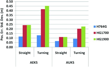
Figure 5. Position errors of CBGS according to different IMUs and filtering/smoothing methods (control updates every 2 points).

Figure 6. Position errors of CBGS according to different IMUs and filtering/smoothing methods (control updates every third point).

Figure 7. Position error of CBGS according to different IMUs and NN aided filtering/smoothing method (control updates every 2 points).

Figure 8. Position error of CBGS according to different IMUs and NN aided filtering/smoothing method (control updates every third point).
Similar to the two-point update case, in every three-point update case the H764G achieved the best position accuracy; and, the nonlinear, adaptive filter/smoothing techniques demonstrated better performance than the AEKS. However, compared to the first case, there was less difference with both methods (AEKS and AUKS) between the straight and turning segments because the accumulation of IMU errors overwhelmed the superiority of the nonlinear filter in a dynamic environment. On the other hand, the non-linear filter still achieves better estimates of states in an essentially non-linear system.
The overall position accuracy was improved by including the neural network aiding, and the disparity in performance between straight and turning sections was reduced. It is noted that the position error of the NN-AEKS decreased dramatically compared to the AEKS in both straight and curved section. The H764G with NN-aided adaptive filtering/smoothing can achieve the area-mapping position requirement (5 cm) along straight sections with eight seconds between updates. Similar results were obtained with the longer interval between updates (every third control point). The position error (st. dev.) of the H764G is less than 10 cm in this case, but in particular, the HG1700 and HG1900 yielded only slightly worse results (1~3 cm more in standard deviation). With the increased interval between control points the NN-aided adaptive filter/smoother was able to maintain the position accuracy better than the unaided adaptive filter/smoother.
4. CONCLUSIONS
For precise geolocation to support UXO detection and characterization, various ranging systems such as GPS, laser, radio, or acoustic ranging can be employed. However, all such systems share limitations or are subject to degradation due to signal occlusions by intervening structures, vegetation, or terrain. In addition, some systems, like GPS, have relatively low temporal resolution. Integration with an inertial measurement unit attempts to overcome, or at least ameliorate these limitations by bridging potential gaps in the ranging solution and increasing the resolution of the geolocation solution. Appropriate integration filters and smoothers are needed to account for the non-linear nature of the system error dynamics, as well as the unknown characteristics of the error statistics. In this paper, both non-linear Kalman filters/smoothers and adaptations based on neural network aiding were studied for the local precise geolocation of UXO detectors.
Laboratory tests were conducted using IMUs with different capabilities and along trajectories with different dynamics. The positioning performance was evaluated for linear and non-linear, as well as adaptive and neural-network-aided adaptive Kalman filter/smoothers. As expected, the nonlinear smoothers, developed from a combination of adaptive unscented Kalman filter and RTS smoother (AUKS) yields superior performance over the standard adaptive extended Kalman smoother.
Each neural-network-aided adaptive filter/smoother improved the overall positioning accuracy for both benign and more dynamic trajectory segments of the test. The navigation-grade IMU (H764G) achieved the area-mapping accuracy level (5 cm) required for UXO detection and discrimination along straight segments and control gaps of eight seconds. However, the medium grade IMUs (HG1700 and HG1900) performed well (~10 cm) under the same circumstances and using the NN-aided adaptive non-linear filter/smoother (NN-AUKS). In addition, the neural-network aiding tends to decrease the difference in performance between benign and dynamic components of the trajectory.
ACKNOWLEDGMENTS
This study was supported by SERDP project MM-1565, contracts W912HQ-07-P-0013 and W912HQ-08-C-0044.


