


1. Introduction
Rayleigh–Taylor instability (RTI) develops when light fluids accelerate heavy fluids (Rayleigh Reference Rayleigh1883; Taylor Reference Taylor1950), then bubbles (the light fluid penetrating the heavy one) and spikes (the heavy fluid penetrating the light one) arise, and turbulence is finally induced. A similar phenomenon is observed in Richtmyer–Meshkov instability (RMI), which occurs when an interface separating two kinds of fluids is impulsively accelerated by a shock wave (Richtmyer Reference Richtmyer1960; Meshkov Reference Meshkov1969). Both instabilities play essential roles in various industrial and scientific fields, such as inertial confinement fusion (ICF) (Lindl et al. Reference Lindl, Landen, Edwards, Moses and Team2014) and supernova explosion (Kuranz et al. Reference Kuranz2018). For example, RMI occurs when the shocks generated by intense lasers or X-rays interact with the ablator layer or the fuel layer of an ICF capsule. RMI determines the seed of RTI during the implosion in ICF. Finally, the mixing induced by RMI and RTI significantly reduces and even eliminates the thermonuclear yield. In addition, the shocks generated by star collapse in a supernova interact with the multi-layer heavy elements throughout interstellar space. The mixing induced by RMI and RTI shapes the filament structures in the remnant of the historical supernova of 1054 AD. Therefore, it is significant to investigate the RMI and RTI involved in the interaction of a shock wave and a finite-thickness fluid layer. However, most previous work has focused on the evolution of a single-mode interface with a semi-infinite thickness induced by these two instabilities (Sharp Reference Sharp1984; Brouillette Reference Brouillette2002; Zhou Reference Zhou2017a, Reference Zhoub; Zhai et al. Reference Zhai, Zou, Wu and Luo2018; Banerjee Reference Banerjee2020).
Theoretically, Taylor (Reference Taylor1950) was the first to consider the RTI of a finite-thickness liquid layer and found that the interface-coupling effect is significant when the fluid-layer thickness is sufficiently small. Subsequently, Ott (Reference Ott1972) proposed a nonlinear solution describing the RTI of a thin massless fluid layer and explained the formation of bubbles and spikes. Mikaelian (Reference Mikaelian1982, Reference Mikaelian1985, Reference Mikaelian1990, Reference Mikaelian1995, Reference Mikaelian1996) deduced linear solutions for quantifying the perturbation growths induced by RTI and RMI on an arbitrary number of stratified fluids. If the number of stratified fluids is larger than three, it is difficult to infer the analytical solutions. Jacobs et al. (Reference Jacobs, Jenkins, Klein and Benjamin1995) considered the RMI of a heavy fluid layer and deduced a linear model for the perturbation growth rates at two sides of the fluid layer and a vortex model for the mixing width growth of the fluid layer. Wang et al. (Reference Wang, Guo, Wu, Ye, Liu, Zhang and He2014) analysed the RTI of a fluid layer in a vacuum and proposed a third-order weakly nonlinear solution for the perturbation growths on two sides of the fluid layer. Subsequently, Liu et al. (Reference Liu, Li, Yu, Fu, Wang, Wang and Ye2018b) discussed the RMI of two superimposed fluid layers in a vacuum and inferred a third-order weakly nonlinear solution for the middle-interface perturbation growth.
Experimentally, Jacobs et al. (Reference Jacobs, Klein, Jenkins and Benjamin1993) adopted the gas curtain technique to investigate the shock-induced evolution of a thin  $\textrm {SF}_6$ gas layer and observed three specific flow patterns. Budzinski, Benjamin & Jacobs (Reference Budzinski, Benjamin and Jacobs1994) concluded that the three distinct flow patterns are ascribed to different perturbation amplitudes at two sides of the fluid layer. Jacobs et al. (Reference Jacobs, Jenkins, Klein and Benjamin1995) found it difficult to predict or control the flow pattern because the initial shape of the gas curtain is not controllable. Prestridge et al. (Reference Prestridge, Vorobieff, Rightley and Benjamin2000) measured the circulation on a shocked gas curtain and validated the vortex model proposed by Jacobs et al. (Reference Jacobs, Jenkins, Klein and Benjamin1995). Recently, shock-induced inclined
  $\textrm {SF}_6$ curtain evolution was explored (Olmstead et al. Reference Olmstead, Wayne, Yoo, Kumar, Truman and Vorobieff2017; Romero et al. Reference Romero, Poroseva, Vorobieff and Reisner2021), and it was found that the pressure waves inside the heavy gas are responsible for the scale selection in fully three-dimensional initial conditions, resulting in the Kelvin–Helmholtz instability (KHI) becoming dominant. The soap-film technique was recently utilised to study the interaction of a converging shock wave and a heavy or light fluid layer (Ding et al. Reference Ding, Li, Sun, Zhai and Luo2019; Li et al. Reference Li, Ding, Si and Luo2020; Sun et al. Reference Sun, Ding, Zhai, Si and Luo2020). Compared with the planar RMI, the additional geometric convergent effect (Bell Reference Bell1951; Plesset Reference Plesset1954) and Rayleigh–Taylor stabilisation (RTS) effect induced by high pressures near the focusing point (Luo et al. Reference Luo, Zhang, Ding, Si, Yang, Zhai and Wen2018), introduced by the cylindrical or spherical RMI, complicate the analysis on the fluid-layer evolution. Our previous work (Liang et al. Reference Liang, Liu, Zhai, Si and Wen2020a) extended the soap-film technique and investigated the RMI of five kinds of
  $\textrm {SF}_6$ gas layers in the planar geometry. Except for examining the conclusion of Budzinski et al. (Reference Budzinski, Benjamin and Jacobs1994) that amplitudes of the two interfaces determine the flow patterns, Liang et al. (Reference Liang, Liu, Zhai, Si and Wen2020a) discovered that the rarefaction waves (RW) reflected from the second interface induce the additional RTI of the first interface, which coincides with previous numerical studies (de Frahan, Movahed & Johnsen Reference de Frahan, Movahed and Johnsen2015).
Although significant progress in the study of shock-induced fluid-layer evolution has been made, the influence of the fluid-layer thickness on the layer evolution has not been experimentally studied because the realisation of such experiments is difficult. For example, the fluid-layer thickness is normally fixed by the gas-curtain generation device. However, the fluid-layer thickness could be used advantageously to minimise the amount of mixing and spike penetration in ICF capsules (Drake Reference Drake2018), and an appropriate thickness of the fluid layer even results in the freeze-out of the first interface perturbation growth (Mikaelian Reference Mikaelian1996). Therefore, it is very desirable to investigate the influence of the fluid-layer thickness on the layer evolution, especially when the fluid layer is thin and the interface-coupling effect is prominent. Previous studies (de Frahan et al. Reference de Frahan, Movahed and Johnsen2015; Liang et al. Reference Liang, Liu, Zhai, Si and Wen2020a) only considered the RW but ignored the compression waves (CW) inside a heavy fluid layer. As a result, previous studies only recognised the instability induced by the RW but neglected the CW stabilisation effect involved in the shock-induced heavy-fluid-layer evolution. In this work, to establish a general one-dimensional (1-D) theory for describing the wave patterns and interface motions, we first experimentally investigate the interaction of a shock wave and three kinds of quasi-1-D  $\textrm {SF}_6$ gas layers by varying the fluid-layer thickness. Then, to explore the interfacial instabilities at both sides of a fluid layer, we experimentally study the interaction of a shock wave with six kinds of quasi-two-dimensional (2-D)
  $\textrm {SF}_6$ gas layers with different fluid-layer thicknesses and amplitude combinations. Linear and nonlinear theories will be established to describe the perturbation growths induced by various interfacial instabilities at both sides of the heavy fluid layer. We will explore the shock-induced light-fluid-layer evolution in a future study.
2. Experimental method
To create an  $\textrm {SF}_6$ gas layer, the extended soap-film technique is utilised to generate two shape-controllable and discontinuous interfaces, mainly eliminating the additional short-wavelength perturbations, diffusion layer and three-dimensionality (Liu et al. Reference Liu, Liang, Ding, Liu and Luo2018a; Liang et al. Reference Liang, Zhai, Ding and Luo2019). As shown in figure 1(a), three transparent devices with a width of 140 mm and a height of 10 mm are first manufactured using transparent acrylic sheets with a thickness of 3 mm. The adjacent boundaries of the middle device are carefully engraved to be of a sinusoidal shape with a depth of 1.8 mm. Four thin filaments with a height of 2.0 mm are attached to the inner surfaces of the upper and lower plates at two sides of the middle device in order to restrict the soap film. In this way the filament bulges in the flow field with only 0.2 mm height and its influence on the flow is limited (Liang et al. Reference Liang, Liu, Zhai, Si and Wen2020a). Before the interface formation, the filaments are properly wetted by a soap solution with a mass fraction of 78 % distilled water, 2 % sodium oleate and 20 % glycerine. First, a small rectangular frame with moderate soap solutions dipped on its borders is pulled along the sinusoidal filaments on both sides of the middle device, and two soap-film interfaces are generated and the closed space is formed. Second,
  $\textrm {SF}_{6}$ is pumped into the closed space through an inflow hole to discharge air inside through an outflow hole. An oxygen concentration detector is placed at the outflow hole to ensure the
  $\textrm {SF}_6$ purity inside the closed space. Subsequently, the inflow and outflow holes are sealed. Finally, the left and right transparent devices are gently connected to the middle device, and the combined one is inserted into the test section of a shock-tube.

Figure 1. Schematics of (a) the soap-film interface generation and (b) the initial configuration studied in the present work. Here  $L_0$ denotes the fluid-layer thickness,
  $\textrm {II}_1$ denotes the initial first interface,
  $\textrm {II}_2$ denotes the initial second interface and IS denotes the incident shock wave.
In the Cartesian coordinate system, as sketched in figure 1(b), the perturbations on the two interfaces are single mode as  $y=a_{n}^0\cos (kx)$ within the range of
  $x\in [-60,60]\ \mathrm {mm}$, where
  $a_{n}^0$ denotes the initial amplitude of the
  $n$th interface with
  $n=1$ and 2 and
  $k$ the wavenumber of the two interfaces. In this work,
  $k=104.7\ \textrm {m}^{-1}$, while
  $a_{1}^{0}$ and
  $a_{2}^{0}$ in all cases are listed in table 1. The initial thickness of a fluid layer (
 $L_0$) is defined as the distance between the average positions of the initial first interface (
 $\textrm {II}_1$) with the initial second interface (
 $\textrm {II}_2$). In all, we investigate three kinds of quasi-1-D
  $\textrm {SF}_6$ gas layers with no perturbations and six kinds of quasi-2-D
  $\textrm {SF}_6$ gas layers with three fluid-layer thicknesses and two amplitude combinations. Here, we define the three cases (i.e. cases L10-IP, L30-IP and L50-IP) with
  $a_2^0>0$ as in-phase cases and the three cases (i.e. cases L10-AP, L30-AP and L50-AP) with
  $a_2^0<0$ as anti-phase cases. To minimise the wall effect of the shock tube on the interface evolution, a short flat part with 10 mm on each side of the two interfaces is adopted. Its influence on the interface evolution is limited (Luo et al. Reference Luo, Liang, Si and Zhai2019). The surrounding gas outside the fluid layer is air. The test gas inside the fluid layer is a mixture of
  $\textrm {SF}_6$ and air, and the mass fraction of
  $\textrm {SF}_6$ is
  $0.97\pm 0.01$. The incident shock wave (IS) travels from left to right.
Table 1. Initial physical parameters of an  $\textrm {SF}_6$ fluid layer for different cases. Here,
  $a_{1}^0$ (
 $a_{2}^0$) represents the initial amplitude of the first (second) interface.

The ambient pressure and temperature are 101.3 kPa and  $295.5\pm 1.0$ K, respectively. The Mach number of the IS is
  $1.20\pm 0.01$, the velocity of the IS (
 $u_s$) is
  $412\pm 2\ \textrm {m}\ \textrm {s}^{-1}$, the speed of the transmitted shock (
 $\textrm {TS}_1$) after the IS passes the
  $\textrm {II}_1$, i.e.
  $u_{t1}$, is
  $188\pm 2\ \textrm {m}\ \textrm {s}^{-1}$, the speed of the transmitted shock (
 $\textrm {TS}_2$) after the
  $\textrm {TS}_1$ passes the
  $\textrm {II}_2$, i.e.
  $u_{t2}$, is
  $406\pm 2\ \textrm {m}\ \textrm {s}^{-1}$. Based on the 1-D gas dynamics theory (Han & Yin Reference Han and Yin1993), the jump speed of the first interface (
 $\Delta u_{1}$) is
  $72\pm 1\ \textrm {m}\ \textrm {s}^{-1}$, and the jump speed of the second interface (
 $\Delta u_{2}$) is
  $94\pm 1\ \textrm {m}\ \textrm {s}^{-1}$. Here, we define the Atwood number of gas layer (
 $A$) as
  $(\rho _2-\rho _1)/(\rho _2+\rho _1)$ with
  $\rho _1$ and
  $\rho _2$ the density of air outside the fluid layer and the test gas inside the fluid layer, respectively.
  $A$ equals
  $0.63\pm 0.01$ in this work. The flow field is monitored by high-speed schlieren photography. The high-speed video camera (FASTCAM SA5, Photron Limited) is 60 000 f.p.s. with a shutter time of
  $1 \ \mathrm {\mu }\textrm {s}$. The spatial resolution of schlieren images is
  $0.4 \ \textrm {mm}\ \textrm {pixel}^{-1}$. The flow-field visualisation is limited within the range of
  $x\in [-50,50]\ \mathrm {mm}$, as shown in figure 1(b).
3. Results and discussion
3.1. Quasi-1-D experimental results and analysis
Schlieren images of the shock-induced quasi-1-D  $\textrm {SF}_6$ gas layer evolution are shown in figures 2(a)–2(c) for
  $L_0=10$, 30 and 50 mm, respectively. The moment when the IS impacts the average position of
  $\textrm {II}_1$ is defined as
  $t=0$. Taking the L50-1D case as an example, the wave patterns and interface motions are discussed in detail. After the IS impacts the
  $\textrm {II}_1$, the
  $\textrm {TS}_1$ is generated, and the shocked first interface (
 $\textrm {SI}_1$) begins to move forwards (
 $58\ \mathrm {\mu }\textrm {s}$). Then the
  $\textrm {TS}_1$ impacts the
  $\textrm {II}_2$ (
 $274 \ \mathrm {\mu }\textrm {s}$), and the
  $\textrm {TS}_2$ moves outside the fluid layer followed by the shocked second interface (
 $\textrm {SI}_2$). Meanwhile, the RW is reflected inside the fluid layer and moves towards the
  $\textrm {SI}_1$ (
 $458\ \mathrm {\mu }\textrm {s}$), because the second interface is a slow/fast interface relative to the RW motion. Subsequently, the RW impacts and accelerates the
  $\textrm {SI}_{1}$. Meanwhile, the CW is reflected inside the fluid layer (
 $658\ \mathrm {\mu }\textrm {s}$) and moves towards the
  $\textrm {SI}_2$ because the first interface is a slow/fast interface relative to the CW motion. Later, the CW impacts and accelerates the
  $\textrm {SI}_2$. After the CW passes the
  $\textrm {SI}_2$, the waves reflected inside the fluid layer are feeble and therefore ignored in this work. Finally, all waves refract outside the fluid layer and the interfaces at two sides of the fluid layer move with the same speed (
 $958\ \mathrm {\mu }\textrm {s}$). Notably, owing to the limited
  $L_0$ in the L10-1D case, the two interfaces coalesce to one at a late time (
 $958\ \mathrm {\mu }\textrm {s}$).

Figure 2. Schlieren images of the shock-induced quasi-1-D  $\textrm {SF}_6$ gas-layer evolution in cases (a) L10-1D, (b) L30-1D and (c) L50-1D. Here
  $\textrm {SI}_1$ (
 $\textrm {SI}_2$) denotes the shocked first (second) interface,
  $\textrm {TS}_1$ denotes the transmitted shock after the IS impacts the
  $\textrm {II}_1$ and
  $\textrm {TS}_2$ denotes the transmitted shock after the
  $\textrm {TS}_1$ impacts the
  $\textrm {II}_2$. Numbers denote time in microseconds.
The interface displacements ( $x_{SI_n}$) and velocities (
 $u_{SI_n}$) of the two interfaces are measured from experiments (
 $n=1$ for the first interface and
  $n=2$ for the second interface), as shown in figures 3(a) and 3(b), respectively. We measure the positions of the top, middle and bottom points of both interfaces from each schlieren image and calculate the average value of the three-point positions as the interface position. The pixel size of schlieren images introduces the experimental measurement uncertainty, which is 0.4 mm in this work. The size of error bars equals the size of symbols representing the experimental results. Time is scaled as
  $tu_{t1}/L_0$, interface displacement is scaled as
  $(x_{SI_n}-x_{01})/L_0$ with
  $x_{01}$ the initial position of the first interface and interface velocity is scaled as
  $u_{SI_n}/\Delta u_1$, respectively. The dimensionless displacements and velocities of the first (second) interface converge in all
  $L_0$ cases, especially the interface velocity increment of the first (second) interface during the interaction of the RW (CW) with the first (second) interface, which indicates that we can establish a general 1-D theory applicable to an arbitrary fluid-layer thickness to describe the behaviour of the two interfaces.

Figure 3. The dimensionless displacements (a) and velocities (b) of the first interface (solid symbols) and the second interfaces (hollow symbols). Black, yellow and purple solid (dash-dotted) lines represent the 1-D theory predictions for the first (second) interface in stages I, II and III, respectively. The light blue zones in the insets indicate the interaction of the RW (CW) with the  $\textrm {SI}_1$ (
 $\textrm {SI}_2$). The black dashed lines in the insets represent the scale of measurement error.
First, we define the specific times when the RW and CW are initially generated as  $t^0_{r}$ and
  $t^0_{c}$, the time when the RW impacts the
  $\textrm {SI}_1$ as
  $t^*_{r}$ and the time when the CW impacts the
  $\textrm {SI}_2$ as
  $t^*_{c}$, as sketched in figure 4, respectively. Then
  $t^0_{r}$,
  $t^0_{c}$,
  $t^*_{r}$ and
  $t^*_{c}$ can be calculated as
 \begin{equation} \left.\begin{gathered} t^0_r=\frac{L_0}{u_{t1}},\\ t^0_c=t^*_r=t^0_r+\frac{L_0(1-\Delta u_1/u_{t1})}{c_1},\\ t^*_c=t^*_r+\frac{L_0}{c_1^*}\left[1-\frac{\Delta u_1}{u_{t1}}-\frac{(1-\Delta v_1/v_{t1})(\Delta u_2-\Delta u_1)}{c_1}\right], \end{gathered}\right\} \end{equation}
where  $c_1$ and
  $c^*_1$ are the sound speeds of the test gas between the
  $\textrm {SI}_1$ with
  $\textrm {TS}_1$, and between the
  $\textrm {SI}_2$ with the RW tail, respectively. Based on 1-D gas dynamics theory (Han & Yin Reference Han and Yin1993),
  $c_1$ and
  $c^*_1$ are
  $148\pm 1\ \textrm {m}\ \textrm {s}^{-1}$ and
  $146\pm 1\ \textrm {m}\ \textrm {s}^{-1}$, respectively. Then
  $t^0_{r}$,
  $t^0_{c}$,
  $t^*_{r}$ and
  $t^*_{c}$ are derived in all cases, as listed in table 2. As
  $L_0$ increases,
  $t^0_{r}$,
  $t^0_{c}$,
  $t^*_{r}$ and
  $t^*_{c}$ increase. However, the dimensionless times, i.e.
  $t^0_{r}v_{t1}/L_0$,
  $t^0_{c}v_{t1}/L_0$,
  $t^*_{r}v_{t1}/L_0$ and
  $t^*_{c}v_{t1}/L_0$, equal 1.00, 1.78, 1.78 and 2.68 in all cases, which indicates that the motions of waves inside the fluid layer are not influenced by the fluid-layer thickness.

Figure 4. Sketches of (a) the interaction of  $\textrm {TS}_1$ and
  $\textrm {II}_2$, (b) the interaction of the RW and
  $\textrm {SI}_1$ and (c) the interaction of the CW and
  $\textrm {SI}_2$. Here,
 $c_1$ represents the sound speed of the test gas between the
  $\textrm {SI}_1$ with
  $\textrm {TS}_1$,
  $c_1^*$ denotes the sound speed of the test gas between the
  $\textrm {SI}_2$ with RW tail,
  $c_5$ denotes the sound speed of air after the IS impacts
  $\textrm {II}_1$,
  $p_1$ denotes the pressure of the flow behind the
  $\textrm {TS}_1$,
  $p_2$ denotes the pressure of the flow behind the RW and
  $p_3$ denotes the pressure of the flow behind the CW tail.
Table 2. Physical parameters of an  $\textrm {SF}_6$ fluid layer calculated by the 1-D theory established in this work (3.4) and (3.5). Here
  $t^0_r$ (
 $t^0_c$) denotes the time when RW (CW) is initially generated,
  $t^*_r$ (
 $t^*_c$) denotes the time when the RW (CW) impacts the first (second) interface,
  $L_r$ (
 $L_c$) denotes the streamwise length of the RW (CW) at
  $t^*_r$ (
 $t^*_c$),
  $\delta t_r$ (
 $\delta t_c$) denotes the interaction time of the RW (CW) with the first (second) interface,
  $\overline {g_r}$ (
 $\overline {g_c}$) denotes the average acceleration imposed on the first (second) interface by the RW (CW) and
  $t_r^+$ (
 $t_c^+$) denotes the time when the RW (CW) tail leaves the first (second) interface. The units for time, length and acceleration are microseconds, millimetres and
  $10^6\ \mathrm {m}\ \mathrm {s}^{-2}$, respectively.

Second, as sketched in figure 4, we define the streamwise length of the RW when its head impacts  $\textrm {SI}_1$ as
  $L_r$, the streamwise length of the CW when its head impacts
  $\textrm {SI}_2$ as
  $L_c$, the interaction time of the RW with
  $\textrm {SI}_1$ as
  $\delta t_r$, the interaction time of the CW with
  $\textrm {SI}_2$ as
  $\delta t_c$, the average acceleration that the RW imposes on the
  $\textrm {SI}_1$ as
  $\overline {g_r}$ and the average acceleration that the CW imposes on the
  $\textrm {SI}_2$ as
  $\overline {g_c}$, respectively. Notably, although the acceleration imposed by the RW on the
  $\textrm {SI}_1$ during
  $\delta t_r$, and the acceleration imposed by the CW on the
  $\textrm {SI}_2$ during
  $\delta t_c$ are not constant (Morgan et al. Reference Morgan, Cabot, Greenough and Jacobs2018; Liang et al. Reference Liang, Zhai, Luo and Wen2020b), to simplify the analysis, the accelerations are taken as constant (Morgan, Likhachev & Jacobs Reference Morgan, Likhachev and Jacobs2016; Liang et al. Reference Liang, Liu, Zhai, Si and Wen2020a), which can be regarded as a first-order approximation. To calculate the
  $L_r$,
  $L_c$,
  $\delta t_r$,
  $\delta t_c$,
  $\overline {g_r}$ and
  $\overline {g_c}$, the final velocity (
 $u_{fn}$) of the fluid layer, i.e. the speed of the
  $\textrm {SI}_1$ after the RW accelerates it, should be derived at first. Based on 1-D gas dynamics theory (Velikovich & Phillips Reference Velikovich and Phillips1996; Liang et al. Reference Liang, Zhai, Luo and Wen2020b),
 \begin{equation} u_{fn}=\Delta u_1-\frac{2c_1}{\gamma_1-1}\left[p_{21}^{(\gamma_1-1)/2\gamma_1}-1\right]+ \frac{\sqrt{2}c_1(p_{31}/p_{21}-1)}{\sqrt{\gamma_1(\gamma_1+1)p_{31}/p_{21}}}, \end{equation}
where  $\gamma _1$ is the specific heat ratio of the test gas inside the fluid layer and equals 1.1,
  $p_{21}$ is the ratio of the pressure of the flow behind the
  $\textrm {TS}_2$ (
 $p_2$) to the pressure of the flow behind the
  $\textrm {TS}_1$ (
 $p_1$), as sketched in figure 4 and which equals 0.85. The only unknown parameter
  $p_{31}$, i.e. the ratio of the pressure of the flow behind the CW tail (
 $p_3$) to
  $p_1$, satisfies
 \begin{equation} \frac{c_5}{c_1}=\frac{\gamma_5-1}{p_{31}^{(\gamma_5-1)/2\gamma_5}-1}\left\{\frac{2}{\gamma_1-1} \left[p_{21}^{(\gamma_1-1)/2\gamma_1}-1\right]-\frac{\sqrt{2}(p_{31}/p_{21}-1) p_{21}^{(\gamma_1-1)/2\gamma_1}}{\sqrt{(\gamma_1+1)\gamma_1p_{31}/p_{21}+(\gamma_1-1)\gamma_1}}\right\}, \end{equation}
where  $c_5$ is the sound speed of air after the IS impacts
  $\textrm {II}_1$ and equals
  $369\pm 2\ \textrm {m}\ \textrm {s}^{-1}$ and
  $\gamma _5$ is the specific heat ratio of air and equals 1.4. Then the
  $p_{31}$ and
  $u_{fn}$ can be calculated as 0.90 and
  $101\pm 1\ \textrm {m}\ \textrm {s}^{-1}$ by solving (3.2) and (3.3). Subsequently, we can deduce the expressions for
  $L_r$,
  $\delta t_r$ and
  $\overline {g_r}$ as
 \begin{equation} \left.\begin{gathered} L_r=\frac{L_0(1-\Delta u_1/u_{t1})(\gamma_1+1)(\Delta u_2-\Delta u_1)}{2c_1},\\ \delta t_r=\frac{2L_r}{\gamma_1(\Delta u_1-\Delta u_2)+u_{fn}-\Delta u_1+2c_1},\\ \overline{g_r}=\frac{u_{fn}-\Delta u_1}{\delta t_r}. \end{gathered}\right\} \end{equation}
In this work, because the waves reflected inside the fluid layer after the CW impacts the  $\textrm {SI}_2$ are ignored, the sound speed of the test gas between the
  $\textrm {SI}_1$ with the CW tail equals
  $c_1^*$, as sketched in figure 4(c). Then the expressions for
  $L_c$,
  $\delta t_c$ and
  $\overline {g_c}$ are
 \begin{equation} \left.\begin{gathered} L_c=\delta t_r\left[u_{fn}+c_1^*+\frac{1}{2}(\Delta u_1-\Delta u_2)\right]-(t_c^*-t_r^*)(u_{fn}-\Delta u_2)-\frac{1}{2}\overline{g_r}(\delta t_r)^2,\\ \delta t_c=\frac{2L_c}{(u_{fn}-\Delta u_2)+2c_1^*},\\ \overline{g_c}=\frac{u_{fn}-\Delta u_2}{\delta t_c}. \end{gathered}\right\} \end{equation}
The values of  $L_r$,
  $L_c$,
  $\delta t_r$,
  $\delta t_c$,
  $\overline {g_r}$ and
  $\overline {g_c}$ are listed in table 2. As
  $L_0$ increases,
  $L_r$,
  $L_c$,
  $\delta t_r$ and
  $\delta t_c$ increase, but
  $\overline {g_r}$ and
  $\overline {g_c}$ decrease, which indicates the strengths of the RW and CW become weaker.
In summary, we establish a general 1-D theory to describe the motions of the first interface and second interface in three stages. For the first interface: (I) uniform motion with  $\Delta u_1$ during
  $t^*_r>t>0$; (II) acceleration with
  $\overline {g_r}$ during
  $t_r^+>t>t^*_r$ with
  $t_r^+=t^*_r+\delta t_r$ and (III) uniform motion with
  $u_{fn}$ during
  $t>t_r^+$. For the second interface: (I) uniform motion with the
  $\Delta u_2$ during
  $t^*_c>t>t^0_r$, (II) acceleration with
  $\overline {g_c}$ during
  $t_c^+>t>t^*_c$ with
  $t_c^+=t^*_c+\delta t_c$, and (III) uniform motion with
  $u_{fn}$ during
  $t>t^*_c+\delta t_c$. The values of
  $t_r^+$ and
  $t_c^+$ are listed in table 2. The predictions of the 1-D theory for the interface motions in stages I, II and III are marked with black, yellow and purple lines, respectively, as represented with solid lines for the first interface and dash-dotted lines for the second interface in figures 3(a) and 3(b), which agree well with the experimental results.
3.2. Quasi-2-D experimental results and analysis
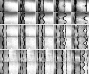
Schlieren images of six kinds of the shock-induced quasi-2-D  $\textrm {SF}_6$ fluid-layer evolution are shown in figures 5(a)–5(f). Except for the actual timescale, we also provide a dimensionless timescale, i.e.
  $\tau _R$ (
 ${=}kv_1^Rt$, in which
  $v_1^R$ is the Richtmyer growth rate calculated with (3.6)). Taking the L30-IP case as an example, the deformations of the two interfaces are discussed in detail. After the IS impacts the perturbed
  $\textrm {II}_1$, the perturbation on the
  $\textrm {SI}_1$ grows, and a rippled
  $\textrm {TS}_1$ moves towards
  $\textrm {II}_2$ (
 $58\ \mathrm {\mu }\textrm {s},\ \tau _R=0.05$). After the
  $\textrm {TS}_1$ impacts the perturbed
  $\textrm {II}_2$, the rippled RW is reflected inside the fluid layer and moves towards
  $\textrm {SI}_1$ (
 $258\ \mathrm {\mu }\textrm {s},\ \tau _R=0.21$). Meanwhile, the perturbation on
  $\textrm {SI}_2$ decreases gradually owing to the phase reversal process (Brouillette Reference Brouillette2002). Subsequently, after the RW impacts
  $\textrm {SI}_1$, the rippled CW is reflected inside the fluid layer and moves towards
  $\textrm {SI}_2$, and the perturbation on
  $\textrm {SI}_2$ nearly disappears at
  $389\ \mathrm {\mu }\textrm {s}$,
  $\tau _R=0.32$). Later, the perturbation on
  $\textrm {SI}_2$ increases with the phase opposite to
  $\textrm {SI}_1$ (
 $673\ \mathrm {\mu }\textrm {s},\ \tau _R=0.56$). Finally, vortices appear on the spike of
  $\textrm {SI}_1$ (
 $956\ \mathrm {\mu }\textrm {s},\ \tau _R=0.79$), which are ascribed to the KHI. The final phase of the
  $\textrm {SI}_2$ in the three in-phase cases is opposite to that of the
  $\textrm {SI}_1$, whereas the final phase of the
  $\textrm {SI}_2$ in the three anti-phase cases is the same as that of the
  $\textrm {SI}_1$. The two interfacial deformations in the L50-IP and L50-AP cases are similar to the corresponding L30-IP and L30-AP cases. Nevertheless, the late-time interface morphologies of the two interfaces in the L10-IP and L10-AP cases are different from the other four large
  $L_0$ cases. In the L10-IP case at
  $959\ \mathrm {\mu }\textrm {s}$ (
 $\tau _R=0.79$), bubbles of the two interfaces coalesce while spikes grow oppositely with their sizes much smaller than the other four large
  $L_0$ cases. In the L10-AP case at
  $965\ \mathrm {\mu }\textrm {s}$ (
 $\tau _R=0.80$), all structures of the two interfaces coalesce. The whole fluid layer evolves into a ‘sinuous’ shape, which qualitatively agrees with the shock-induced gas-curtain morphology reported previously (Jacobs et al. Reference Jacobs, Klein, Jenkins and Benjamin1993; Budzinski et al. Reference Budzinski, Benjamin and Jacobs1994; Jacobs et al. Reference Jacobs, Jenkins, Klein and Benjamin1995).

Figure 5. Schlieren images of the shock-induced quasi-2-D  $\textrm {SF}_6$ fluid-layer evolution in cases (a) L10-IP, (b) L10-AP, (c) L30-IP, (d) L30-AP, (e) L50-IP and (f) L50-AP. Numbers denote time in microseconds.
The amplitudes of the first and second interfaces,  $a_1$ and
  $a_2$, are defined as half of the streamwise distance between the spike tip with the bubble tip of the first interface and second interface, respectively. We measure the positions of two bubble tips and one spike tip of the first interface from each schlieren image, and calculate the
  $a_1$ by the average of two bubble tip positions minus the spike tip position. We measure the positions of two bubble (spike) tips and one spike (bubble) tip of the second interface in the three in-phase (anti-phase) cases from each schlieren image, and calculate the
  $a_2$ by the average of two bubble (spike) tip positions minus the spike (bubble) tip position. The amplitude growths on the two interfaces are divided into three stages based on the 1-D theory established in this work: I. Linear stage (
 $t^*_r>t>0$ for the first interface,
  $t^*_c>t>t^0_r$ for the second interface), II. Early nonlinear stage (
 $t^+_r>t>t^*_r$ for the first interface,
  $t^+_c>t>t^*_c$ for the second interface) and III. Late nonlinear stage (
 $t>t^+_r$ for the first interface,
  $t>t^+_c$ for the secondinterface).
In the linear stage, only RMI decides the amplitude growths of the two interfaces. The linear growth rates of the amplitude of the two interfaces,  $v_1^{exp}$ and
  $v_2^{exp}$, are acquired by linear fitting the two interface amplitudes measured from experiments, as listed in table 3. For cases with the same
  $L_0$, the
  $v_1^{exp}$ and
  $v_2^{exp}$ are larger in the three anti-phase cases than those in the three in-phase cases. For cases with the same amplitude combinations, as the
  $L_0$ increases, the
  $v_1^{exp}$ and
  $v_2^{exp}$ increase in the three in-phase cases, but decrease in the three anti-phase cases. In order to determine the difference between the classical RMI of a semi-infinite single-mode interface with the RMI of a heavy fluid layer, the Richtmyer impulsive theory (Richtmyer Reference Richtmyer1960) is adopted to calculate the first interface amplitude growth rate (
 $v_1^R$), and the Meyer–Blewett impulsive theory (Meyer & Blewett Reference Meyer and Blewett1972) is utilised to obtain the second interface amplitude growth rate (
 $v_2^{MB}$) as
 \begin{equation} \left.\begin{gathered} v_1^R=Z_1a_1^0k\Delta u_1A,\\ v_2^{MB}={-}\frac{(Z_2+1)a_2^0k\Delta u_2A}{2}, \end{gathered}\right\} \end{equation}
with two compression factors  $Z_1=1-\Delta u_1/v_s$ and
  $Z_2=1-\Delta u_2/v_{t1}$. The values of
  $v_1^R$ and
  $v_2^{MB}$ in all cases are listed in table 3. Here
  $v_1^{exp}$ is smaller than
  $v_1^R$ in the three in-phase cases, and
  $v_2^{exp}$ is larger than
  $v_2^{MB}$ in the three anti-phase cases. The difference between the experimental result and the corresponding theoretical result is pronounced when
  $L_0$ is limited, which agrees with previous findings (Ott Reference Ott1972). As a result, the coupling between the two interfaces of a fluid layer, i.e. the interface-coupling effect, plays a vital role in influencing RMI development (Jacobs et al. Reference Jacobs, Jenkins, Klein and Benjamin1995; Mikaelian Reference Mikaelian1996; Liang et al. Reference Liang, Liu, Zhai, Si and Wen2020a), especially when the initial fluid-layer thickness is small.
Table 3. The amplitude growth rates of the two interfaces in different cases. Here,  $v_1^{exp}$ (
 $v_2^{exp}$) denotes the linear amplitude growth rate of the first (second) interface measured from experiments,
  $v_1^{R}$ (
 $v_2^{MB}$) denotes the linear amplitude growth rate of the first (second) interface calculated with the Richtmyer (Meyer–Blewett) impulsive theory (3.6),
  $v_1^{l}$ (
 $v_2^{l}$) denotes the linear amplitude growth rate of the first (second) interface calculated with the mJ model (3.9) and (3.10a,b) and
  $v_{1b/1s}^{+}$ (
 $v_{2b/2s}^{+}$) denotes the early nonlinear bubble/spike amplitude growth rate of the first (second) interface at
  $t_r^+$ (
 $t_c^+$) calculated with the mZG model (3.11) and (3.12). The unit for velocity is
  $\textrm {m}\ \mathrm {s}^{-1}$.

Jacobs et al. (Reference Jacobs, Jenkins, Klein and Benjamin1995) introduced a linear solution (J model) for describing the amplitude growth rates of the first interface ( $v_1^l$) and second interface (
 $v_2^l$) by considering the interface-coupling effect on the RMI,
 \begin{equation} \left.\begin{gathered} v_1^l=\frac{k\Delta u_1\left[A_t(a_1^0-a_2^0)+A_c(a_1^0+a_2^0)\right]}{2},\\ v_2^l=\frac{k\Delta u_2\left[A_t(a_1^0-a_2^0)-A_c(a_1^0+a_2^0)\right]}{2}, \end{gathered}\right\} \end{equation}
with two modified Atwood numbers,
 \begin{equation} A_t=\frac{\rho_2-\rho_1}{\rho_2\tanh(kL_0/2)+\rho_1}\quad \mathrm{and}\quad A_c=\frac{\rho_2-\rho_1}{\rho_2\coth(kL_0/2)+\rho_1}. \end{equation}
When  $L_0\rightarrow \infty$,
  $A_t=A_c=A$ and the J model reduces to the Richtmyer impulsive theory. Notably, the amplitude growth rate of one interface is influenced by the initial amplitude of the other interface, which indicates the interface-coupling effect. The J model adopts the pre-shock parameters and ignores the shock compression effect. Here, we modify the J model for the first interface by considering the IS compression and for the second interface by considering the
  $\textrm {TS}_1$ compression. Then the modified J model (mJ model) can be expressed as
 \begin{equation} \left.\begin{gathered} v_1^l=\frac{k\Delta u_1\left\{A_t\left[Z_1a_1^0-(Z_2+1)a_2^0/2\right]+A_c\left[Z_1a_1^0+(Z_2+1)a_2^0/2\right]\right\}}{2},\\ v_2^l=\frac{k\Delta u_2\left\{A_t\left[Z_1a_1^0-(Z_2+1)a_2^0/2\right]-A_c\left[Z_1a_1^0+(Z_2+1)a_2^0/2\right]\right\}}{2}, \end{gathered}\right\} \end{equation}
with two new modified Atwood numbers,
 \begin{equation} A_t=\frac{\rho_2-\rho_1}{\rho_2\tanh(Z_LkL_0/2)+\rho_1}\quad \mathrm{and} \quad A_c=\frac{\rho_2-\rho_1}{\rho_2\coth(Z_LkL_0/2)+\rho_1}, \end{equation}
where a new compression factor  $Z_L=1-\Delta u_1/v_{t1}$ is introduced. The values of
  $v_1^l$ and
  $v_2^l$ are listed in table 3, which agree well with the experimental results. As a result, the mJ model is applicable for describing the interface-coupling effect on the RMI in the linear stage.
The time-varying nonlinear amplitudes of the two interfaces are shown in figures 6(a) and 6(b), respectively. For the first interface, the time is scaled as  $\tau _1=kv_1^l(t-t_r^*)$, and the amplitude is scaled as
  $\eta _1=k(a_1-a_1^*)$ with
  $a_1^*$ the amplitude of the first interface at
  $t_r^*$. For the second interface, the time is scaled as
  $\tau _2=k|v_2^l|(t-t_c^*)$ and the amplitude is scaled as
  $\eta _2=k(|a_2|-|a_2^*|)$ with
  $a_2^*$ the amplitude of the second interface at
  $t_c^*$. The predictions of the mJ model, as shown with black lines in figures 6(a) and 6(b), underestimate the dimensionless
  $a_1$ but overestimate the dimensionless
  $a_2$ when
  $\tau _1>0$ and
  $\tau _2>0$, respectively. Therefore, the interaction of the RW with the first interface leads to the first interface being more unstable, and the interaction of the CW with the second interface results in the second interface being more stable. In addition, for the first interface, the dimensionless
  $a_1$ converges in all cases, which indicates that the fluid-layer thickness and amplitude combinations have limited influence on the nonlinear behaviour of the first interface perturbation growth. For the second interface, although the dimensionless
  $a_2$ converges in the four large
  $L_0$ cases, the dimensionless
  $a_2$ in the two
  $L_0=10$ mm cases are different and larger than the other four large
  $L_0$ cases at a late time, which indicates that the nonlinear behaviour of the second interface perturbation growth is influenced by the amplitude combination and the fluid-layer thickness when the
  $L_0$ is limited.

Figure 6. Comparisons of the dimensionless amplitudes of (a) the first interface and (b) the second interface. Black, yellow and purple lines represent the theoretical predictions for two interface amplitudes in the linear stage (3.9) and (3.10a,b), early nonlinear stage (3.11)–(3.15) and late nonlinear stage (3.16)–(3.18), respectively. The black dashed lines in the insets represent the scale of measurement error.
In the early nonlinear stage, during the interaction of the RW and the first interface, as sketched in figure 7(a), the light fluids outside the fluid layer accelerate the heavy fluids inside the fluid layer, which leads to the additional RTI of the first interface. In contrast, during the interaction of the CW and the second interface, the heavy fluids inside the fluid layer accelerate the light fluids outside the fluid layer, leading to the additional RTS of the second interface. The additional RTI increases the amplitude growth rate of the first interface (de Frahan et al. Reference de Frahan, Movahed and Johnsen2015; Liang et al. Reference Liang, Liu, Zhai, Si and Wen2020a) but the additional RTS decreases the amplitude growth rate of the second interface. Here, we modify the ZG model Zhang & Guo (Reference Zhang and Guo2016) by considering the universal curves of all spikes and bubbles at any density ratio, to quantify the additional RTI of the first interface and the additional RTS of the second interface. To simplify the analysis, we consider that the RTI of the first interface and the RTS of the second interface are induced by the 1-D RW and CW, respectively. Then the expressions of the modified ZG model, i.e. the mZG model, for the first interface bubble/spike amplitude growth rate ( $v_{1b/1s}^{en}$) and the second interface bubble/spike amplitude growth rate (
 $v_{2b/2s}^{en}$) are
 \begin{equation} \left.\begin{gathered} \frac{\mathrm{d}v_{1b/1s}^{en}}{\mathrm{d}t}={-}\alpha_{b/s}k\left[(v_{1b/1s}^{en})^{2}-(v_{1b/1s}^{qs})^2\right],\\ \frac{\mathrm{d}v_{2b/2s}^{en}}{\mathrm{d}t}=\frac{a_2^0}{|a_2^0|}\alpha_{b/s}k\left[(v_{2b/2s}^{en})^{2}-(v_{2b/2s}^{qs})^2\right], \end{gathered}\right\} \end{equation}
with
 \begin{equation} \left.\begin{gathered} v_{1b/1s}^{qs}=\sqrt{\frac{A\overline{g_{r}}}{3k}\frac{8}{(1\pm A)(3\pm A)}\frac{\left[3\pm A+\sqrt{2(1\pm A)}\right]^{2}}{\left[4(3\pm A)+\sqrt{2(1\pm A)}(9\pm A)\right]}},\\ v_{2b/2s}^{qs}=\sqrt{\frac{A\overline{g_{c}}}{3k}\frac{8}{(1\pm A)(3\pm A)}\frac{\left[3\pm A+\sqrt{2(1\pm A)}\right]^{2}}{\left[4(3\pm A)+\sqrt{2(1\pm A)}(9\pm A)\right]}}, \end{gathered}\right\} \end{equation}
and
 \begin{equation} \alpha_{b/s}=\frac{3}{4}\frac{(1\pm A)(3\pm A)}{\left[3\pm A+\sqrt{2(1\pm A)}\right]}\frac{\left[4(3\pm A)+\sqrt{2(1\pm A)}(9\pm A)\right]}{\left[\sqrt{3\pm A}+2\sqrt{2(1\pm A)}(3\mp A)\right]}. \end{equation}
The upper (lower) sign of  $\pm$ and
  $\mp$ in all equations of this work applies to the bubble (spike). Note that the interface-coupling effect is considered because the initial
  $v_{1b/1s}^{en}$ equals
  $v_1^l$ at
  $t^*_r$, and the initial
  $v_{2b/2s}^{en}$ equals
  $v_2^l$ at
  $t^*_c$. The final bubble/spike amplitude growth rates of the two interfaces at the end of the early nonlinear stage, i.e. the bubble/spike amplitude growth rate of the first interface (
 $v_{1b/1s}^{+}$) at
  $t_r^+$, and the bubble/spike amplitude growth rate of the second interface (
 $v_{2b/2s}^{+}$) at
  $t_c^+$, are calculated with the mZG model (3.11) and (3.12), as listed in table 3. The differences between
  $v_{1b/1s}^{+}$ with
  $v_1^l$ are prominent in all cases, which indicates the effect of the RTI induced by the RW on the first interface perturbation growth is essential, regardless of a large or small fluid-layer thickness. The differences between
  $v_{2b/2s}^{+}$ with
  $v_2^l$ are prominent when the
  $L_0$ is limited, which indicates as the fluid-layer thickness decreases, the RTS induced by the CW plays an increasingly important role on influencing the second interface perturbation growth.

Figure 7. Sketches of (a) the interaction of the RW with  $\textrm {SI}_1$ and (b) the interaction of the CW with
  $\textrm {SI}_2$.
In addition, the RW firstly accelerates the bubble, then the spike of the first interface, as shown in figure 7(a). The direction of the acceleration that the RW imposes on the bubble is the same as the bubble amplitude growth. Hence, the RW decompresses the bubble before it impacts the spike of the first interface. The streamwise distance between the bubble tip with the spike tip of the first interface is  $2a_1^*$, the relative velocity between the first interface and the RW head is
  $c_1$, and the first interface speed increment induced by the RW is (
 $u_{fn}-\Delta u_1$). Therefore, the time-varying RW decompression effect on the first interface bubble amplitude (
 $a_r$) is
 \begin{equation} a_r=\frac{(u_{fn}-\Delta u_1)(t-t_r^*+a_1^*/c_1)}{2}, \end{equation}
with  $(t_r^*+a_1^*/c_1)>t>(t_r^*-a_1^*/c_1)$. The CW also first accelerates the bubble, then the spike of the second interface, as shown in figure 7(b). However, the direction of the acceleration that the CW imposes on the bubble is the opposite of the bubble amplitude growth. Hence the CW compresses the bubble before it impacts the spike of the first interface. The streamwise distance between the bubble tip with the spike tip of the second interface is
  $2a_2^*$, the relative velocity between the second interface and the CW head is
  $c_1^*$, and the second interface speed increment induced by the CW is (
 $u_{fn}-\Delta u_2$). Therefore, the time-varying CW compression effect on the second interface bubble amplitude (
 $a_c$) is
 \begin{equation} a_c={-}\frac{(u_{fn}-\Delta u_2)(t-t_c^*+a_2^*/c_1^*)}{2}, \end{equation}
with  $(t_c^*+a_2^*/c_1^*)>t>(t_c^*-a_2^*/c_1^*)$.
Based on the previous analysis, it is concluded that in the early nonlinear stage, the first interface evolution is dominated by the RMI, RTI and the decompression induced by the RW; and the second interface evolution is dominated by the RMI, RTS and the compression caused by the CW. The prediction for the  $a_1$ by considering the additional RTI using the ZG model and the decompression induced by the RW, as shown with yellow lines in figure 6(a), agrees well with all experimental results. The prediction for the
  $a_2$ by considering the additional RTS using the ZG model and the compression induced by the CW, as shown with yellow lines in figure 6(b), agrees well with all experimental results except for the two cases with
  $L_0=10$ mm. In the L10-IP and L10-AP cases, the CW impacts the second interface before the end of the phase reversal of the second interface owing to the limited
  $L_0$. Therefore, the decrement of the dimensionless
  $a_2$ in the early nonlinear stage is mainly ascribed to the phase reversal process imposed by the RMI.
In the late nonlinear stage, after the RW tail leaves the first interface, the first interface moves with a constant speed, and therefore only the RMI dominates the first interface evolution. Similarly, after the CW tail leaves the second interface, only the RMI dominates the second interface evolution. Because the amplitudes of the two interfaces,  $a_1^+$ and
  $a_2^+$, at the end of the early nonlinear stage violate the small-amplitude prerequisite (i.e.
  $ka_1^+\ll 1$ and
  $|ka_2^+|\ll 1$), the high-amplitude effect on the nonlinear behaviour of the RMI development is non-negligible. Here, we modify the DR model (Dimonte & Ramaprabhu Reference Dimonte and Ramaprabhu2010) by considering various amplitude-wavelength ratios and density ratios to describe the late nonlinear RMI in this study. The expressions of the modified DR model, i.e. mDR model, for the first interface bubble/spike amplitude growth rate (
 $v_{1b/1s}^{ln}$) and the second interface bubble/spike amplitude growth rate (
 $v_{2b/2s}^{ln}$) are
 \begin{equation} \left.\begin{gathered} v_{1b/1s}^{ln}=\frac{v_{1b/1s}^{+}\left[1+(1\mp A)kv_{1b/1s}^{+}t\right]}{1+C_{1b/1s}kv_{1b/1s}^{+}t+(1\mp A)F_{b/s}(kv_{1b/1s}^{+}t)^2},\\ v_{2b/2s}^{ln}=\frac{v_{2b/2s}^{+}\left[1+(1\mp A)k|v_{2b/2s}^{+}|t\right]}{1+C_{2b/2s}k|v_{2b/2s}^{+}|t+(1\mp A)F_{b/s}(k|v_{2b/2s}^{+}|t)^2}, \end{gathered}\right\} \end{equation}
with
 \begin{equation} \left.\begin{gathered} C_{1b/1s}=\frac{4.5\pm A+(2\mp A)ka_{1b/1s}^+}{4},\\ C_{2b/2s}=\frac{4.5\pm A+(2\mp A)k|a_{2b/2s}^+|}{4}, \end{gathered}\right\} \end{equation}
and
 \begin{equation} F_{b/s}=1\pm A. \end{equation}
The mDR model predictions for  $a_1$ and
  $a_2$ are shown in figures 6(a) and 6(b) with purple lines, respectively, and agree well with all experimental results for the first interface, and the four large
  $L_0$ cases for the second interface. As the RTI and decompression effect induced by the RW promote the first interface perturbation growth, and the RTS and compression effect caused by the CW suppress the second interface perturbation growth, the
  $a_1$ is larger than the
  $a_2$ in all cases. In addition, bubbles of the two interfaces coalesce in the L10-IP case, and all structures of two interfaces combine in the L10-AP case at a late time, as shown in figures 5(e) and 5(f). As a result, the second interface perturbation growths are promoted by the first interface counterpart in the L10-IP and L10-AP cases, and which exceed the mDR model predictions. Overall, the
  $a_2$ in the L10-IP and L10-AP cases is smaller than the
  $a_1$ but larger than the mDR model prediction.
4. Conclusions
Experimental and theoretical studies on an air/ $\textrm {SF}_6$/air fluid layer with a finite thickness have been performed to investigate the wave patterns, interface motions and interfacial instabilities of both sides of a fluid layer. Experimentally, the extended soap-film technique has been utilised in a shock tube to create three kinds of quasi-1-D layers with different layer thicknesses, and six kinds of quasi-2-D layers with diverse layer thicknesses and amplitude combinations. We have adopted schlieren photography and have used a high-speed camera to capture experimental pictures. The RW and CW going back and forth inside fluid layers have been identified.
First, wave patterns and interface motions in the three quasi-1-D heavy-fluid-layer cases have been studied. The RW reflected from the second interface accelerates the first interface, and the CW reflected from the first interface accelerates the second interface. Finally, all waves refract outside the fluid layer and the two interfaces of the fluid layer move with a same speed. A general 1-D theory is established to describe the two interfaces’ motions in three stages: (I) uniform motion with the post-shock velocity, (II) acceleration induced by the RW or CW and (III) uniform motion with the final speed.
Second, the morphologies of the two interfaces of a quasi-2-D heavy fluid layer induced by a shock wave are investigated. The final phase of the second interface is opposite of that of the first interface when the initial amplitudes of the two interfaces are the same, whereas the final phase of the second interface is the same as that of the first interface when the initial amplitudes of the two interfaces are the opposite. For the first time, it is observed experimentally that local or whole structures of the two interfaces coalesce when the initial fluid layer is very thin.
Third, the interfacial instabilities of a quasi-2-D heavy fluid layer are examined, which can be divided into three stages. (I) Linear stage. Before the RW impacts the first interface, or before the CW impacts the second interface, only the RMI dominates the perturbation growth of the first interface, or the second interface. (II) Early nonlinear stage. During the interaction of the RW and the first interface, the RMI, the RTI and the decompression effect induced by the RW dominate the first interface perturbation growth. During the interaction of the CW and the second interface, the RMI, the RTS and the compression effect induced by the CW dominate the second interface perturbation growth. The RW destabilises the first interface, but the CW stabilises the second interface. (III) Late nonlinear stage. After the RW passes the first interface, or after the CW passes the second interface, only the RMI dominates the perturbation growth of the first interface, or the second interface.
Fourth, linear and nonlinear models are successfully established by considering the interface-coupling effect on the RMI, and the additional interfacial instabilities induced by these waves inside the heavy fluid layer. The linear amplitude growths of the two interfaces can be well described by the mJ model considering the interface-coupling effect and the post-shock parameters. The early nonlinear perturbation growth on the first interface can be characterised by the sum of the mZG model prediction for quantifying the additional RTI and the decompression effect on the first interface bubble amplitude. The early nonlinear perturbation growth on the second interface can be described by a sum of the mZG model prediction for quantifying the additional RTS and the compression effect on the second interface bubble amplitude. The late nonlinear perturbation growths on the two interfaces can be characterised by the mDR model. As local or whole structures of the first interface and second interface coalesce and the amplitude growth rate of the first interface is larger than that of the second interface, the nonlinear perturbation growth of the second interface of a thin fluid layer is promoted by the first interface counterpart and exceeds the mDR model prediction. It is worth looking forward to testing the proposed models in this study with more experiments by varying the shock strengths, amplitudes, wavenumbers and phases of the perturbations on the two interfaces.
Funding
This work was supported by Tamkeen under the NYU Abu Dhabi Research Institute grant CG002 and the Natural Science Foundation of China (grant numbers 11772329, 91952205 and 11625211). The authors are grateful to Dr L. Liu's help on performing experiments.
Declaration of interests
The authors report no conflict of interest.


