


U.S. corporate defined benefit pension plans have received considerable recent attention from both practitioners and academic researchers, and for good reason. Pension assets are substantial, averaging roughly 1/6 of total firm value. Among about 2,000 firms that sponsor defined benefit plans, average total plan assets exceed $1,500 billion and average total projected benefit obligations exceed $1,600 billion.
In addition to the importance conveyed by their size, corporate pension plans involve some interesting and complex financial contracts. One long-standing issue is the question ‘Who owns the assets in a defined benefit pension plan?’ (Bulow and Scholes, Reference Bulow, Scholes, Bodie and Shoven1983). Prior to the passage of the Employee Retirement Income Security Act (ERISA) in 1974, pension liabilities were not liabilities of the firm. At plan termination, beneficiaries or employees had claims on the assets of the pension fund, but no claims on other corporate assets. However, under ERISA, pension assets and liabilities are treated as corporate assets and liabilities; this is explicitly recognized by the Financial Accounting Standards Board (FASB) in its statement SFAS 87. On the other hand, ERISA shifted some of the firm's contingent obligations onto the government, specifically the Pension Benefit Guaranty Corporation (PBGC). If the company is in distress and pension funding is inadequate to support promised retirement benefits, the PBGC's insurance program guarantees those benefits up to specified limits. This implicit put option implies that the government has a stake in – and implicit property rights to – the firm's pension assets and liabilities.
A number of empirical studies (Oldfield, Reference Oldfield1977; Feldstein and Seligman, Reference Feldstein and Seligman1981; Feldstein and Morck, Reference Feldstein, Morck, Bodie and Shoven1983; Daley, Reference Daley1984; Dhaliwal, Reference Dhaliwal1986; Landsman, Reference Landsman1986; Bodie et al., Reference Bodie, Light, Morck, Taggart, Bodie, Shoven and Wise1987; Bulow et al., Reference Bulow, Morck, Summers, Bodie, Shoven and Wise1987; Barth, Reference Barth1991) have attempted to infer the implicit property rights to pension plan assets and liabilities. These studies commonly entail regressions of firm value on pension plan assets and liabilities. The typical empirical question is whether the estimated coefficients on pension assets or liabilities in firm valuation regressions are close to 1.0 in absolute value. Feldstein and Seligman (Reference Feldstein and Seligman1981) find that while each dollar increase in pension liabilities reduces equity value by about a dollar, a corresponding increase in pension assets increases equity value by less than a dollar. These results support the hypothesis that stock market investors treat the liabilities, but not the assets, of pension plans as fully internalized by the firm. This is consistent with the view that firms are responsible for underfunded liabilities but may have difficulty in accessing assets of overfunded plans for general corporate purposes. However, a more recent study by Liébana and Vincent (Reference Liébana and Vincent2004) finds no consistent evidence that investors value firms' pension assets and liabilities as though they belonged to the sponsoring firms. The valuation implications of pension plans remain unanswered.
Unlike earlier studies, we explicitly consider in this paper the implications of the firm's financial health on the valuation effects of pension plan funding. To the extent that firms may eventually walk away from their obligations, other parties (e.g., the PBGC as well as incompletely insured employees) may be partial claimants on the assets and liabilities of the plan. This will attenuate the response of firm value to pension funding. We therefore distinguish among firms based on their financial condition.
Firms may behave strategically in allocating pension assets and choose to ‘go for broke’ (Harris and Raviv, Reference Harris and Raviv1992) when they approach financial distress to maximize the value of the PBGC put option. Besides increasing the total value of the pension put, such risk-shifting behavior can reallocate the values of the contingent claims (and liabilities) across the various stakeholders.Footnote 1
Moreover, flexible actuarial choices make pension valuation soft and discretionary (Scholes and Wolfson, Reference Scholes, Wolfson, Scholes and Wolfson1992). Several papers show that firms' actuarial choices, such as pension discount rate, cost method, and the forecast salary growth rate vary with the financial condition of the firm (Morris et al., Reference Morris, Nichols and Niehaus1983; Bodie et al., Reference Bodie, Light, Morck, Taggart, Bodie, Shoven and Wise1987; Ghicas, Reference Ghicas1990; Gopalakrishnan and Sugrue, Reference Gopalakrishnan and Sugrue1995; Godwin et al., Reference Godwin, Goldberg and Duchac1996; Petersen, Reference Petersen, Fernandez, Turner and Hinz1996; Asthana, Reference Asthana1999). As a general rule, firms appear to choose conservative pension assumptions in good times and aggressive ones in bad times. All these factors, i.e., the PBGC put option, strategic risk-taking, and discretionary actuarial choices, call for pension valuation models that are conditioned on financial status.
We capture the level and change in firms' financial conditions over consecutive fiscal years using bankruptcy-risk scores developed in three studies: Ohlson (Reference Ohlson1980), Altman (Reference Altman1968), and Campbell et al. (Reference Campbell, Hilscher and Szilagyi2008). We use Ohlson_BS, Altman_Z, and CHS_BS to denote the corresponding bankruptcy scores and ΔOhlson_BS, ΔAltman_Z, and ΔCHS_BS to denote changes in firms' financial status between consecutive fiscal years. (In all cases, we add minus signs to the changes in bankruptcy-risk scores, so that positive numbers indicate improvements in financial condition.)
Taking Ohlson's (Reference Ohlson1980) bankruptcy score as an example, we use the estimated parameters from his model to calculate Ohlson_BS for each firm in our sample. Then, we compute the difference between the Ohlson_BS during consecutive fiscal years. The resulting ΔOhlson_BS index measures the change in firms' financial condition. Depending on whether ΔOhlson_BS is positive or negative, we partition firms into healthier versus more distressed groups and estimate a pension valuation model for the two groups. We ask how changes in various items on the pension fund balance sheet affect changes in the market valuation of the firm, and whether those valuation effects depend on the firm's financial status.
Aside from conditioning valuation effects on financial status, the other major novelty in our approach is a focus on the changes in market value that result from changes in pension funding. Earlier studies have focused almost exclusively on the level of plan assets and obligations. The valuation measures employed by these studies typically include the ratio of market value to book value of assets (Tobin's Q), the ratio of market value to book value of equity (M/B), or the market value of equity normalized by other deflators. However, these multiples, which are used to assess the impact of pension funding on the market valuation of the firm, are relatively crude benchmarks. Moreover, because levels of balance sheet items are highly persistent from year to year, time series variation in pension funding and financial condition does not provide much power to tease out corresponding variation in valuation multiples, especially given the imprecision in the benchmarks.
Our focus on changes rather than levels offers several advantages. First, changes in stock market value are observed as contemporaneous rates of return, and we have a rich set of tools to net out the impact of broad market movements to obtain cleaner estimates of the firm-specific return in any period. By controlling more precisely for benchmark returns, we enhance the signal-to-noise ratio and improve the power of our empirical tests. Second, an excess-return valuation method allows for an adjustment for the difference in risk factors and, therefore, the difference in discount rates on firm valuation (Faulkender and Wang, Reference Faulkender and Wang2006).
Third, whereas variation in pension funding may have only a second-order impact on valuation multiples, they are far more telling for changes in market value. Changes in pension net funding will have a far greater proportional impact on equity value (which will show up as an excess return) than on variation in any valuation multiple.Footnote 2 Therefore, we adopt a long-run benchmark-adjusted stock return approach, as in Grinblatt and Moskowitz (Reference Grinblatt and Moskowitz2004) and Faulkender and Wang (Reference Faulkender and Wang2006). The dependent variable is a stock's excess return relative to the matched size and book-to-market portfolio of Fama and French (Reference Fama and French1992, Reference Fama and French1993).
The focus on changes rather than levels poses one potential problem in interpretation. For consistency with our other variables, we partition firms based on change in financial status, but are ultimately interested in the difference between healthy and distressed firms. However, we demonstrate that changes in bankruptcy scores display considerable serial correlation: on average, strengthening firms in 1 year continue to strengthen in the following year, and weakening firms continue to weaken. Therefore, it would be reasonable for the market to conclude that firms with currently worsening financial metrics are more likely to encounter serious challenges in the future, and therefore present a higher likelihood of offloading pension obligations onto other parties. Moreover, when we partition on the level of distress score, we obtain results broadly consistent with, albeit less powerful than, results based on partitions using changes.
We summarize our major results as follows. First, using all firm-year observations from June 1988 to June 2017, we find the following point estimates, given in the ‘All firms’ column, for the impact on firm value changes in various pension assets or liabilities:

These results thus offer new evidence suggesting that pension fund assets and liabilities are valued by the market much less than one-for-one. Moreover, the market seems to value an extra dollar of accumulated benefit obligations more highly than an extra dollar of projected benefit obligations. Investors seem to recognize off-balance sheet pension liabilities as well. Not only is the estimate large in magnitude, but the significance level is high.
Second, the valuation impact of pension funding differs considerably by financial health. The three columns to the right show that for all three indices of financial strength, the valuation effects for healthier firms are greater than those for the entire sample of firms. This result suggests that pension funding has stronger valuation effects on financially secure firms.
In contrast, for firms that have become financially weaker, valuation effects (not shown in this excerpt) are much smaller; in fact in the majority of cases, they are statistically indistinguishable from zero. Below, we present formal tests of the hypothesis that the valuation effects are the same for healthy and distressed stocks. We firmly reject the null hypothesis for each of the five pension asset and liability variables above, regardless of which distress-risk score is used to partition the sample. These patterns are even stronger following the adoption of pension accounting rules that increased disclosure requirements.
While we employ several measures of financial strength, our results are robust to the particular measure used to partition the sample. This is in part because the alternative indices of the evolution of financial status (ΔOhlson_BS, ΔAltman_Z, and ΔCHS_BS) are themselves generally consistent. The pairwise correlations between the three are all positive, ranging from 0.29 to 0.47, and are all statistically significant at better than a 5% level.
Third, both improvements and deterioration in financial health tend to persist. On average, firms in the improving or STRONGER group in 1 year exhibit further reductions in financial risk in the next year. Conversely, firms in the WEAKER group exhibit higher risk in the next year. This pattern implies that forecasts of future financial distress can be sensitive to recent changes in bankruptcy-risk scores. This is consistent with our finding that valuation effects are highly associated with such changes.
Fourth, we estimate the valuation impacts of mandatory contributions to pension plans. While overfunded plans do not have to make contributions, firms operating underfunded plans (for which projected benefit obligations exceed pension assets) are required by law to make catch-up contributions. We construct two measures of mandatory contributions following Moody (2006) and Campbell et al. (Reference Campbell, Dhaliwal and Schwartz2012). The first, Mand1, equals service cost (retirement benefits accrued by plan participants during the year) plus one-thirtieth of current underfunding, measured as the difference between accrued benefits and plan assets. The second, Mand2, is simply that year's service cost. (If either statistic is negative, e.g., due to plan overfunding, the variable is set equal to zero.) The stock market reacts to either measure of mandatory contributions with a sensitivity far exceeding one-for-one. Every incremental dollar of mandatory contributions reduces stock market value by more than $5 for STRONGER firms versus roughly zero to $2 for WEAKER firms. We interpret these results as evidence that a change in mandatory contributions is generally long lasting, and the market discounts the present value of the entire stream of required future contributions. For distressed firms, for which there is a greater likelihood that the stream of contributions will be interrupted, the impact is significantly lower.
Fifth, we find that small firms, which generally are less likely to hedge uncertainty (Nance et al., Reference Nance, Smith and Smithson1993), are more sensitive to variation in pension valuation. We carry out a two-way partition based on both market capitalization and each of the three distress-risk indices. The partition divides all firms into the following four interactive groups: large and healthier, large and more distressed, small and healthier, and small and more distressed. We find the differential valuation effects between healthier and more distressed firms are stronger for small firms than large firms.
Our work is also related to the accounting literature on pension valuation focusing on the relevance of a fair or market value model versus that of a smoothed model under SFAS 87, the pension accounting recognition and measurement rule instituted by the Financial Accounting and Standards Board. The accounting literature is typically based on empirical variants of the Ohlson (Reference Ohlson1995) model that provide a direct link between accounting measures and firm value. These studies include Daley (Reference Daley1984), Landsman (Reference Landsman1986), Barth (Reference Barth1991), Barth et al. (Reference Barth, Beaver and Landsman1992), Coronado and Sharpe (Reference Coronado and Sharpe2003), Coronado et al. (Reference Coronado, Mitchell, Sharpe and Nesbitt2008), and Hann et al. (Reference Hann, Heflin and Subramanyam2007). Glaum (Reference Glaum2009) provides a detailed review of the value relevance of pension accounting information. There is also a growing related literature on the management of pension assumptions and actuarial choices (Thomas, Reference Thomas1988; Thomas and Tung, Reference Thomas and Tung1992; Blankley and Swanson, Reference Blankley and Swanson1995; Amir and Gordon, Reference Amir and Gordon1996; Amir and Benartzi, Reference Amir and Benartzi1998; Bergstresser et al., Reference Bergstresser, Desai and Rauh2006).Footnote 4
The rest of the paper proceeds as follows. Section 1 develops our main hypothesis. Section 2 describes data sources, sample screening, and variable definitions. Section 3 presents summary statistics. Section 4 provides the baseline valuation for corporate pension plans. Section 5 constructs three bankruptcy scores used to develop partitioning indices. Section 6 examines the persistence of firms' changes in financial condition. Section 7 estimates the valuation model for firms' pension assets and liabilities, conditional on recent changes in financial condition. Section 8 examines the conditional valuation of mandatory contributions. Section 9 explores the role of firm size in pension valuation. Finally, Section 10 concludes.
1. Hypothesis development
ERISA has important implications regarding the property rights of corporate pension plans. Since its implementation, researchers have tended to view pension assets as corporate assets and pension liabilities as corporate liabilities (Sharpe, Reference Sharpe1976; Treynor, Reference Treynor1977; Barnow and Ehrenberg, Reference Barnow and Ehrenberg1979; Tepper, Reference Tepper1981; Bulow, Reference Bulow1982). Nevertheless, both are subject to a few important special considerations (Bulow et al., Reference Bulow, Scholes, Menell, Bodie and Shoven1983).
First, ERISA created the PBGC, which insures obligations to plan beneficiaries. If distressed firms terminate their plans, the PBGC pays the difference between (i) the guaranteed benefit and (ii) the assets in the pension funds plus 30% of the firms' net worth. Employers pay insurance premiums against plan termination. Second, ERISA restricts the transfer of pension plan assets to the corporation, making it costly for firms to overfund pension plans and later pull back the funds. In addition, the Tax Reform Act of 1986 introduced an excise tax on reversion of pension plan assets. These considerations imply that the ownership of net pension assets is only partially retained by the firm.
We will focus primarily on the financial status of the firm. Regardless of the current level of pension funding, financially healthy firms cannot simply walk away from pension obligations; the PBGC put comes into play only in the event of bankruptcy. Pension obligations, like other prospective liabilities, are more likely to be internalized by shareholders when the firm is healthier and more likely to honor them, so this is the variable on which we focus. For example, an increase in the value of pension assets due to strong market returns should increase the value of a financially strong firm that is likely to pay its pension obligations by more than the value of a distressed firm that is viewed as likely to renege on those obligations in any event. Therefore, the response of firm value to the value of pension funding should depend on the firm's financial status. This suggests these two hypotheses:
Hypothesis 1
Only a fraction of the change in net pension assets should be internalized in the market's assessment of a firm's intrinsic value.
Hypothesis 2
Pension valuation effects should be stronger for financially healthy firms than for those vulnerable to financial distress.
Nevertheless, conditional on financial distress, pension funding will matter, as shown in Bulow and Scholes (Reference Bulow, Scholes, Bodie and Shoven1983). In practice, of course, pension funding tends to be correlated with financial strength, so these effects are intertwined. We will present evidence on the interaction of these two variables.
2. Data sources, sample screening, and variable definitions
2.1 Data sources and sample stocks
The data for U.S. equity markets are from the CRSP and COMPUSTAT merged files. We obtain monthly returns, monthly stock prices, and market capitalization from CRSP. The annual accounting items, such as fiscal year-end shares outstanding and book value of equity, and pension related variables, such as plan assets and projected benefit obligations, are taken from COMPUSTAT. We use NYSE, AMEX, and NASDAQ firms, excluding financial firms with 4-digit SIC codes between 6000 and 6999.
2.2 Sample period and FASB statements
Our sample period begins in June 1988 when SFAS 87 imposed new standards on pension reporting. SFAS 87 (FASB, 1985) requires that accumulated benefit obligations determine recognition of minimum liability and dictates a smoothed rather than a fair or market-value model for pension accounting. Under SFAS 132 (FASB, 1988), effective in December 1997, firms are no longer required to report separate pension items for over- and under-funded plans. Under SFAS 158, effective as of December 2006 (FASB, 2006), firms must incorporate fair value funding status, or the difference between plan assets and projected benefit obligations, in their consolidated statements. Minimum pension liability adjustments associated with accumulated benefit obligations under SFAS 87 are no longer required. The sample ends in June 2017.
2.3 Variable definitions
Our variables fall into four groups: pension variables, raw and benchmark-adjusted excess stock returns, accounting variables, and financial strength measures. We discuss the first three categories in this section. Pension-plan related variables include plan assets (PA), projected benefit obligations (PBO), accumulated benefit obligations (ABO), funding status (Funding_Status), off-balance sheet items (OFF_BAL), and two measures of mandatory contributions (Mand1 and Mand2). These are all scaled by beginning-of-fiscal-year market capitalization. The details of the construction of these variables are provided in Appendix A. The measures of financial strength are treated in Section 5.
Plan assets (PA) refer to funds set aside to meet a firm's obligations. They increase due to capital gains on existing assets as well as from the difference between firm contributions and benefit payouts. PBO is the present value of employees' projected future benefits, which requires firms to make several actuarial assumptions, for example, concerning number of years until retirement, post-retirement life expectancy, final salary, and the appropriate discount rate. Whereas PBO is based on expected future salaries, ABO calculates employees' future benefits using their current salaries; it is the current value of obligations already earned, and equal to the present value of benefits if the plans were terminated immediately.
Funding_Status is the difference between PA and PBO. According to SFAS 158, this difference must be immediately incorporated into the balance sheet. However, until 2006, U.S. GAAP kept some pension gains and losses off the firm's financial statements to smooth the periodic pension cost. Off-balance-sheet pension assets or liabilities (OFF_BAL) included unrecognized gains and losses (Unreg_GL), unrecognized prior service costs (Unreg_SC), and unrecognized transitional assets and liabilities (Unreg_TAL). Unreg_SC measures retroactive benefits awarded to employees due to plan amendments. COMPUSTAT integrates Unreg_GL and Unreg_TAL together into one number. It estimates changes in PBO due to changes in actuarial assumptions and the deferred gains and losses that result from the difference between expected and actual returns on plan assets.Footnote 5
Following the literature, we control for risk and macroeconomic factor exposure using the 25 size and book-to-market portfolios of Fama and French (Reference Fama and French1992, Reference Fama and French1993). Liew and Vassalou (Reference Liew and Vassalou2000) show that these factors predict GDP growth, and may therefore control for some aspects of business cycle risk. To the extent that market returns depend on interest rate innovations, the FF factors at least partially control for that source of risk as well. Stock i's excess return in year t is its return minus that of the benchmark portfolio to which it belongs at the beginning of the fiscal year. We calculate annual returns (including dividends) for the fiscal year by cumulating monthly returns for both individual stocks and the 25 FF portfolios.
Our regression model for valuation of pension variables incorporates the following ten control variables; for each, we calculate changes between consecutive fiscal years of: cash holdings (CASH); interest expenses (INT); earnings before interest and taxes (EBIT); and non-cash total assets (Non-Cash_Assets). We adjust EBIT for pension cost (PC) by adding back the pension cost that is typically deducted. We also control for beginning-of-period cash holding (CASH t−1); accruals (ACCRUALS); external financing (XFIN), which includes both debt and equity financing; asset growth (ASST_GWTH); market leverage (MLEV); and beginning-of-fiscal year firm size (Mkt_Eq t−1). We deflate the firm-specific factors (except for asset growth, market leverage, and firm size) by the 1-year lagged market value of equity (Mkt_Eq t−1). This standardization enables us to interpret the estimated coefficients as the dollar change in value for a $1 change in the corresponding independent variable. The details of the construction of these variables using COMPUSTAT items are provided in Appendix A.
3. Summary statistics
The sample for NYSE/AMEX/NASDAQ covers 348 months, from June 1988 to June 2017. There are 2,737 stocks for which the necessary pension variables are available in this period. While we have 23,446 firm-year observations for ΔPA, ΔPBO, ΔFunding_Status, and ΔOFF_BAL, there are fewer firm-year observations for ΔABO because disclosure of ABO was not required between 1999 and 2003. The number of firms in our sample in each year ranges from 606 in fiscal year 2016 to 997 in 1994. However, these are not the same firms in each year, so 2,117 distinct firms appear at least once in the sample. Panel A of Table 1 provides summary statistics, including mean, median, 25th and 75th percentile values, and standard deviations. Panel B presents pairwise correlations of key variables.
Table 1. Summary statistics

The sample consists of U.S. firms on the NYSE/AMEX/NASDAQ and the CRSP and COMPUSTAT merge files during the June 1988 to June 2017 period. Panel A reports summary statistics, constructed using pooled firm-year observations. Pension asset and liability related items include changes in the following variables: pension assets (ΔPA), projected benefit obligations (ΔPBO), accumulated benefit obligations (ΔABO), funding status (ΔFunding_Status), and off-balance-sheet pension assets or liabilities (ΔOFF_BAL). Mandatory contributions include two measures, Mand1 and Mand2, following Moody's (2006) and Campbell et al. (Reference Campbell, Dhaliwal and Schwartz2012), respectively. The return variables include the raw returns (R it) and the Fama–French 25 size and book-to-market ratio adjusted returns (R it − R Bt) measured over the corresponding fiscal year. The accounting variables include lagged cash holdings (CASH −1), changes in cash holdings (ΔCASH), changes in interest payments (ΔINT), changes in pension-cost adjusted earnings before interest and taxes (ΔEBIT + PC), changes in non-cash assets (ΔNon-Cash_Assets), the level of accrual (ACCRUALS), the level of external financing (XFIN), asset growth (ASST_GWTH), market leverage (MLEV), and beginning-of-fiscal-year market capitalization (Mkt_Eq −1). Pension variables and accounting variables are all scaled by beginning of the fiscal year market capitalization except for ASST_GWTH and MLEV. The details of the construction of the variables are given in Appendix A. Panel B reports pair-wise correlation coefficients. * and ** indicate significance at the 10% and 5% levels, respectively.
Panel A shows that the average increase in pension assets is 1.6% and the average increase in projected benefit obligations is 1.8%, resulting in an average annual change in funding status of −0.3% of the beginning of the fiscal year market value. The mean annual stock return in excess of the Fama and French (Reference Fama and French1992, Reference Fama and French1993) size and book-to-market adjusted benchmark is 1.4%. This is roughly the same magnitude as the average change in pension-cost adjusted earnings before interest and taxes, 1.7%.
Panel B reveals that ΔPA has significant correlations of 0.43, 0.70, and 0.74, respectively, with ΔPBO, ΔABO, and ΔFunding_Status. ΔABO and ΔPBO are highly correlated (0.81), which is not surprising. However, the positive correlation (0.30) between ΔABO and ΔFunding_Status combined with the negative correlation between ΔPBO and ΔFunding_Status (−0.21) suggests that pension assets track accumulated benefit obligations more closely than projected benefit obligations.
4. Baseline valuation
4.1 Pension assets and liabilities
Table 2 presents estimates of the following baseline valuation model for the entire sample of firms, in which the dependent variable R i,t − R B,i,t is the return of stock i during fiscal year t, net of the return on the benchmark portfolio (matched by size and book-to-market ratio):
 $$\eqalign{R_{i,t}-R_{B,i,t} = & \, \alpha _0 + \alpha _1\Delta Y_{i,t} + \gamma _1\displaystyle{{CASH_{i,t-1}} \over {Mkt\_Eq_{i,t-1}}} + \gamma _2\displaystyle{{\Delta CASH_{i,t}} \over {Mkt\_Eq_{i,t-1}}} + \gamma _3\displaystyle{{\Delta INT_{i,t}} \over {Mkt\_Eq_{i,t-1}}} \cr & + \gamma _4\displaystyle{{\Delta {(EBIT + PC)}_{i,t}} \over {Mkt\_Eq_{i,t-1}}} + \gamma _5\displaystyle{{Non{\rm -}Cash\,Assets_{i,t}} \over {Mkt\_Eq_{i,t-1}}} + \gamma _6\displaystyle{{ACCRUALS_{i,t}} \over {Mkt\_Eq_{i,t-1}}} \cr & + \gamma _7\displaystyle{{XFIN_{i,t}} \over {Mkt\_Eq_{i,t-1}}} + \gamma _8ASST\_{GWTH_{i,t}}\; + \gamma _9MLEV_{i,t} + \gamma _{10}\log (Mkt\_Eq_{i,t-1}) + \varepsilon _{i,t}} $$
The independent variables in equation (1) include the control variables discussed earlier.Footnote 6 The variable of interest is denoted by ΔY, which in each column of Table 2 equals the change in one of the following pension variables respectively: plan assets (ΔPA), projected benefit obligations (ΔPBO), accumulated benefit obligations (ΔABO), funding status (ΔFunding_Status), off-balance sheet pension items (ΔOFF_BAL), and mandatory contributions. The control variables in Table 2 generally exhibit high levels of significance with the expected signs.
Table 2. Stock market valuation of corporate pension plans

Regression estimates of equation (1):
 $$\eqalign{R_{i,t}-R_{B,i,t} = & \,\alpha _0 + {\rm} \alpha _1\Delta Y_{i,t} + \gamma _1\displaystyle{{CASH_{i,t-1}} \over {Mkt\_Eq_{i,t-1}}} + \gamma _2\displaystyle{{\Delta CASH_{i,t}} \over {Mkt\_Eq_{i,t-1}}} + \gamma _3\displaystyle{{\Delta INT_{i,t}} \over {Mkt\_Eq_{i,t-1}}} \cr & + \gamma _4\displaystyle{{\Delta {(EBIT + PC)}_{i,t}} \over {Mkt\_Eq_{i,t-1}}} + \gamma _5\displaystyle{{Non{\rm -}Cash\,Assets_{i,t}} \over {Mkt\_Eq_{i,t-1}}} + \gamma _6\displaystyle{{ACCRUALS_{i,t}} \over {Mkt\_Eq_{i,t-1}}} \cr & + \gamma _7\displaystyle{{XFIN_{i,t}} \over {Mkt\_Eq_{i,t-1}}} + \gamma _8ASST\_{GWTH_{i,t}}\; + \gamma _9MLEV_{i,t} + \gamma _{10}log(Mkt\_Eq_{i,t}_{-1} ) + \varepsilon _{i,t}} $$
The sample consists of U.S. firms on the NYSE/AMEX/NASDAQ and the CRSP and COMPUSTAT merge files during the June 1988 to June 2017 period. The table reports the estimation results for the model in Grinblatt and Moskowitz (Reference Grinblatt and Moskowitz2004) and Faulkender and Wang (Reference Faulkender and Wang2006). The dependent variable is the Fama–French 25 size and book-to-market ratio adjusted return (R it − R Bt). The independent variables include lagged cash holdings (CASH −1), changes in cash holdings (ΔCASH), changes in interest payments (ΔINT), changes in pension-cost adjusted earnings before interest and taxes (Δ(EBIT + PC)), changes in non-cash assets (ΔNon-Cash_Assets), the level of accrual (ACCRUALS), the level of external financing (XFIN), asset growth (ASST_GWTH), market leverage (MLEV), and beginning-of-fiscal-year market value (Mkt_Eq −1). Pension variables and accounting variables are all scaled by beginning-of-fiscal-year capitalization except for ASST_GWTH and MLEV. * and ** indicate significance at the 10% and 5% levels, respectively. Petersen (Reference Petersen2009) and Thompson (Reference Thompson2011) two-dimension firm and year clustered t-statistics are reported.
Because ΔPA is scaled by market capitalization, its coefficient in column (1) implies that each extra dollar of plan assets is valued by shareholders at $0.43, with a t-statistic of 2.27. Similarly, each dollar in other pension items are valued on the margin as follows: projected benefit obligations (ΔPBO), −$0.28, with a t-statistic of −2.41; accumulated benefit obligations (ΔABO), −$0.58, with a t-statistic of −2.06; funding status (ΔFunding_Status), $0.37, with a t-statistic of 2.21; off balance sheet pension items (ΔOFF_BAL), $0.34, with a t-statistic of 1.83. We include industry fixed effects in the ordinary least squares (OLS) regressions; standard errors have been adjusted for clustering in both firm and year (Petersen, Reference Petersen2009; Thompson, Reference Thompson2011).
If the market views the firm as completely responsible for the additional assets and liabilities generated during the fiscal year, then the estimated coefficients should be close to $1.00 for asset-related items and −$1.00 for liability-related items. In fact, the regression coefficients are generally closer to one-half. Investors seem to be most sensitive to changes in accumulated benefit obligations (ΔABO), for which the −$0.58 valuation coefficient is closest to $1.00 in absolute value. The fact that these coefficients are all below 1.0 may reflect in part the fact that the net-of-tax value-impact of pension contributions and reversions would reflect the tax deductibility of such cash flows. However, even allowing for such effects, these coefficients are still considerably below the values one would expect if the firm had full and certain ownership claims and obligations for the pension plan.
The glaring exception is the response to mandatory contributions. The estimates (t-statistics) on Mand1 and Mand2 are −5.03 (−3.37) and −6.37 (−3.54), respectively. This high response superficially suggests market overreaction, but far more likely, it reflects a recognition that any change in mandatory contribution this year signifies a repeated obligation in following years for catch-up funding. Thus, the market appears to be imputing the present value of an annuity of mandatory contributions. In contrast, changes in the other pension fund measures, for example, accrued benefits, would not be expected to be persistent.
In Table 3, we check the robustness of these results by considering five alternative estimation methods. Method 1 employs OLS regressions with year and industry fixed effects. Method 2 employs OLS regressions with year and industry fixed effects, but with t-statistics adjusted for the clustering by firm. Method 3 includes only industry fixed effects. The t-statistics are adjusted for the clustering-in-year effects. Whereas the first three OLS regression methods do not employ firm dummies, method 4 uses a fixed-effect panel regression controlling for both year and firm effects with t-statistics adjusted for clustering by firm. Finally, method 5 employs a random-effect panel regression controlling for year, industry, and firm effects. The t-statistics are adjusted for clustering by firm. Because these OLS and panel regressions all generate similar results, in subsequent analysis, we rely on the simpler OLS approach with standard errors adjusted for clustering by both firm and year, as in Table 2.
Table 3. Alternative regression methods

Alternative regression estimates of equation (1). The sample consists of U.S. firms on the NYSE/AMEX/NASDAQ and the CRSP and COMPUSTAT merge files during the June 1988 to June 2017 period. The dependent variable is the Fama–French 25 size and book-to-market ratio adjusted return (R it − R Bt). The independent variables include lagged cash holdings (CASH −1), changes in cash holdings (ΔCASH), changes in interest payments (ΔINT), changes in pension-cost adjusted earnings before interest and taxes (Δ(EBIT + PC)), changes in non-cash assets (ΔNon-Cash_Assets), the level of accrual (ACCRUALS), the level of external financing (XFIN), asset growth (ASST_GWTH), market leverage (MLEV), and beginning-of-fiscal-year market value (Mkt_Eq −1). Pension variables, including changes in pension assets and liabilities (ΔPA, ΔPBO, ΔABO, ΔFunding_Status, and ΔOFF_BAL), are included one-at-a-time in each equation. Pension variables and accounting variables are all scaled by beginning of the fiscal year market capitalization except for ASST_GWTH and MLEV. * and ** indicate significance at the 10% and 5% levels, respectively.
5. Indices measuring changes in financial conditions
To test Hypothesis 2 (that pension funding effects depend on financial status), we require measures of financial strength. Therefore, we construct three measures to capture the evolution of firms' financial conditions and link that evolution to the valuation of corporate pension plans. Our measures are based on three popular models of bankruptcy risk: Ohlson (Reference Ohlson1980), Altman (Reference Altman1968), and Campbell et al. (Reference Campbell, Hilscher and Szilagyi2008). We use original estimates from these papers, except for the Altman (Reference Altman1968) model, for which we use the updated estimates from Shumway (Reference Shumway2001). Appendix A summarizes the construction of these bankruptcy scores.Footnote 7
5.1 Ohlson (1980) bankruptcy score
Ohlson (Reference Ohlson1980) estimates a static binary logit bankruptcy model. The probability of bankruptcy is modeled as P(X i,β) = [1 + exp(−X iβ)]−1, where X i is a vector of variables constructed from the firm's financial statements observed 1 year before bankruptcy. He finds four factors to be statistically significant for assessing the probability of bankruptcy: size, leverage, performance, and liquidity. The original estimated parameters from model 1 in Table 4 of Ohlson (Reference Ohlson1980) are used to compute Ohlson's bankruptcy score for firm i in fiscal year t:  $Ohlson\_BS_{i,t} = {\rm } \ndash X_{i,t}\hat{\beta} $.Footnote 8
Table 4. Bankruptcy scores and change in financial condition indices
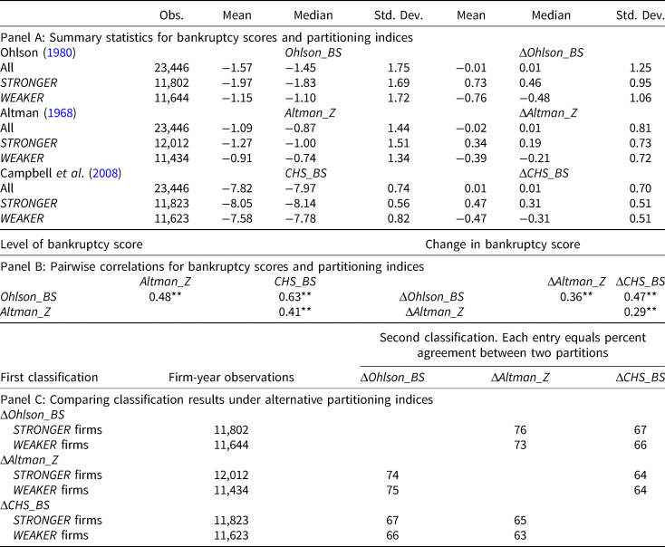
The sample consists of U.S. firms on the NYSE/AMEX/NASDAQ and the CRSP and COMPUSTAT merge files during the June 1988 to June 2017 period. Firms are partitioned into STRONGER and WEAKER groups based on whether annual changes in the following three bankruptcy scores are positive or negative: the Ohlson (Reference Ohlson1980) score (ΔOhlson_BS), the Altman (Reference Altman1968) index (ΔAltman_Z), and the Campbell et al. (Reference Campbell, Hilscher and Szilagyi2008) score (ΔCHS_BS). Panel A tabulates simple summary statistics for bankruptcy scores and partitioning indices for the entire sample and for the STRONGER and WEAKER subgroups of firms. Panel B presents pairwise correlations between bankruptcy scores and partitioning indices, using all firm-year observations. Panel C compares the classification results for STRONGER and WEAKER firms based on the partitioning indices. * and ** indicate significance at the 10% and 5% levels, respectively.
5.2 Altman bankruptcy score
Altman (Reference Altman1968) applies discriminant analysis to a sample of bankrupt and non-bankrupt firms during the 1946–65 period. The following variables best distinguish between these two types of firms: working capital, retained earnings, earnings before interest and taxes, and sales, all scaled by total assets, and the ratio of market value of equity to book value of total debt. Shumway (Reference Shumway2001) updates the estimates using data from 1962 to 1992. We use the estimates in Table 2 of Shumway (Reference Shumway2001) to construct Altman's (Reference Altman1968) Z-score. We also add a negative sign to Z-scores, so that, like our other measures, higher algebraic values indicate riskier firms,  $Altman\_Z_{i,t} = {\rm } \ndash X_{i,t}\hat{\beta} $.
5.3 Campbell, Hilscher, and Szilagyi bankruptcy score
Campbell et al. (Reference Campbell, Hilscher and Szilagyi2008) estimate bankruptcy risk using a multi-period dynamic logit model over the 1963–2003 period. Their model is similar to those of Shumway (Reference Shumway2001) and Chava and Jarrow (Reference Chava and Jarrow2004). The probability of bankruptcy in the next year is computed as P(X i,t−1,β) = [1 + exp(−X i,t−1β)]−1. They identify several variables that are significant in predicting the probability of failure: relative size, lagged stock excess return, volatility, profitability, leverage, and current liquidity. The model is employed to predict 1, 6, 12, 24, and 36-month-ahead probabilities of failure. We use the original estimated coefficients for 1-year-ahead predictions in Table 4 of Campbell et al. (Reference Campbell, Hilscher and Szilagyi2008) to compute the bankruptcy score for firm i during fiscal year t,  $CHS\_BS_{i,t}\; = \ndash X_{i,t}\hat{\beta} $.
5.4 Indices measuring changes in financial conditions
Bankruptcy scores provide measures of each firm's financial condition. A simple INDEX of the change in financial condition over consecutive fiscal years is the difference in the bankruptcy score from t to t − 1. For example, using the Ohlson bankruptcy score measure as the partitioning index:
 $$INDEX_{i,t}\; = \Delta Ohlson\_BS_{i,t}\; = \; -(Ohlson\_BS_{i,t}\; -Ohlson\_BS_{i,t}_- _1)$$
The higher the value of ΔOhlson_BS i,t, the more the firm's financial condition has improved. We construct analogous indexes for the two other bankruptcy scores, thus generating INDEX i,t = ΔAltman_Z i,t and ΔCHS_BS i,t respectively.
We use these indexes to partition firms in each fiscal year into healthier and more distressed groups according to whether the INDEX is positive or negative and create two dummy variables (STRONGER and WEAKER)Footnote 9:
 $$STRONGER_{i,t}\; = \left\{ {\matrix{ 1 & {if\; \;INDEX_{i,t} \gt 0} \cr 0 & {if\; \;INDEX_{i,t} \le 0} \cr}} \right.$$
and
 $$WEAKER_{i,t}\; = \left\{ {\matrix{ 1 & {if\; \;INDEX_{i,t} \le 0} \cr 0 & {if\; \;INDEX_{i,t} \gt 0} \cr}} \right.$$
Our partition generates a roughly equal number of firm-year observations for firms in both the healthier and more distressed groups for each of the three partitioning indices.
Figure 1 shows the mean values of each of these financial health indexes in each year. The figure shows that small funds exhibit noticeably greater variation in the evolution of their financial health: for each measure of financial strength, improving small firms enjoy greater average increases in financial health than improving large firms, and weakening small firms suffer greater average declines in financial health than weakening large firms.

Figure 1. The evolution of indices measuring changes in financial conditions over time. Panel A: ΔOhlson_BS; panel B: ΔAltman_Z; panel C: ΔCHS_BS.
5.5 Consistency of classification
The three partitioning indices, ΔOhlson_BS, ΔAltman_Z, and ΔCHS_BS, each measuring changes in financial conditions, are constructed from historical estimates based on differing statistical models and sample periods. This raises the question of whether the indices generally identify the same set of firm-years as exhibiting improved or worsening financial conditions.
Panel A of Table 4 reports the mean, median, and standard deviation of the three bankruptcy-risk scores (Ohlson_BS, Altman_Z, and CHS_BS) as well as their changes. We report summary statistics for all firms, healthier firms, and more distressed firms, respectively. Panel B reports correlations between bankruptcy scores and between partitioning indices. The correlations between bankruptcy scores range from 0.41 to 0.63. Correlations between the partitioning indices that measure changes in financial conditions range from 0.29 to 0.47. All correlations are significant at better than the 1% level.
Panel C examines the consistency of classification under these alternative partitioning indices. There are a total of 23,446 firm-year observations in our entire sample. Of these, 11,802 and 11,644 are classified as STRONGER and WEAKER, respectively, under the first partitioning index, ΔOhlson_BS. The question is how many of these 11,802 firm-year observations will be similarly classified as STRONGER under the two other partitioning indices. Panel C shows that of the 11,802 STRONGER firm-year observations, 76% and 67% are also classified as STRONGER under ΔAltman_Z and ΔCHS_BS, respectively. Similarly, of the 11,644 firm-year observations classified as WEAKER under ΔOhlson_BS, 73% and 66% are also classified as WEAKER under ΔAltman_Z and ΔCHS_BS, respectively.
The other parts of panel C summarize the classification results when we alternate the first partitioning index and the second partitioning index. Between 64% and 76% of firms identified as STRONGER under the first index remain so under the second index. Between 63% and 75% of firms identified as WEAKER under the first index remain so under the second. We conclude that these measures are largely in agreement.
6. Persistence of firms' financial conditions
The stability of financial ratios may change over time, especially when firms approach bankruptcy (Dambolena and Khoury, Reference Dambolena and Khoury1980). Therefore, in this section, we examine two issues related to the reliability of the bankruptcy scores. First, we compare the information content of their current levels as well as their change over consecutive years. Second, we study the persistence of changes in condition of firms in the STRONGER and WEAKER groups.
6.1 The information content of bankruptcy scores and changes in bankruptcy score
We examine the information content of the level and change in the three alternative bankruptcy scores following the approach in Hillegeist et al. (Reference Hillegeist, Keating, Cram and Lundstedt2004). However, rather than applying these models to predict actual failure during the sample period, we apply them to predict which firms are at risk of entering financial distress. A firm is defined to be at risk of distress in year t + 1 if net income as a percent of beginning-of-fiscal year market value, NI t/Mkt_Eq t−1, is less than −20%. We use ‘at risk of distress’ rather than actual failure because financial distress is sufficient to encourage risk-shifting behavior. This criterion for distress is still demanding: the fraction of firms in our sample that exhibit financial distress according this criterion is small, only 3.45% of the firm-year observations. Our results are robust to alternative cut-off levels of NI t/Mkt_Eq t−1 such as −30%.
We test the 1-year-ahead predictive power for financial distress constructed from alternative bankruptcy scores (BS) using the following logit regression:
 $$P\lpar {At\_Risk_{i,t + 1} = {\rm} 1} \rpar = \displaystyle{{\exp (a_0 + a_1BS_{i,t})} \over {1 + \exp (a_0 + a_1BS_{i,t})}}$$
where At_Risk i,t+1 is a dummy variable that takes the value 1 if firm i in fiscal year t + 1 is at risk of distress and 0 otherwise. Panel A of Table 5 reports logit regressions when current financial conditions measured by the three bankruptcy scores (Ohlson_BS, Altman_Z, and CHS_BS) are used as explanatory variables. Panel B reports estimates when both lagged levels and changes in financial conditions are used as explanatory variables.
Table 5. Predictive power of levels and changes in financial conditions

The sample consists of U.S. firms on the NYSE/AMEX/NASDAQ and the CRSP and COMPUSTAT merge files during the June 1988 to June 2017 period. The table reports the 1-year ahead predictive power of bankruptcy scores (BS) for future firm ‘distress’ in the following logit regression:
 $$P(At\_Risk_{i,t + 1} = 1) = \displaystyle{{{\rm e}^{a_0 + a_1BS_{i,t}}} \over {1 + {\rm e}^{a_0 + a_1BS_{i,t}}}},$$
where At_Risk ,t+1 is a dummy variable that takes the value one if firm i in fiscal year t + 1 is deemed to be in distress and zero otherwise. A firm is defined to be in distress if its net income scaled by beginning-of-fiscal-year market equity is less than −20%. A total of 3.37% of firm-years in our sample exhibit distress. Panel A reports the logit regressions when current levels of financial conditions constructed from three bankruptcy scores (Ohlson_BS, Altman_Z, and CHS_BS) are used as explanatory variables. Panel B reports the logit regressions when both lagged levels and changes in financial conditions are used as explanatory variables. * and ** indicate significance at the 10% and 5% levels, respectively.
By and large, these credit risk scores do predict financial distress over short horizons, with highly significant coefficient estimates. Table 5 shows that the CHS_BS score from the Campbell et al. (Reference Campbell, Hilscher and Szilagyi2008) model has the highest predictive power for financial distress measured by both the R 2 and log-likelihood function, followed by the Altman_Z score and the Ohlson_BS score. The models that use both lagged level and change in scores slightly outperform those that use only the current level of bankruptcy.
6.2 Persistence of changes in firms' financial conditions
We now examine the serial correlation of changes in bankruptcy scores following the method in Ali and Zarowin (Reference Ali and Zarowin1992). In each year, we estimate the following cross-sectional regression for both groups of firms (STRONGER and WEAKER), respectively:
 $$INDEX_{i,t} = c_0 + c_1INDEX_{i,t-1} + \varepsilon _{i,t}$$
where INDEX i,t is one of the three measures capturing the change in firms' financial conditions.Footnote 10 Table 6 partitions firms each year into STRONGER and WEAKER groups based on their change in financial condition (ΔOhlson_BS, ΔAltman_Z, ΔCHS_BS). The table reports the annual average of the intercept and slope coefficients of equation (2) as well as the corresponding Fama and MacBeth (Reference Fama and MacBeth1973) t-statistics for the two partitioned groups. The table also reports the Wilcoxon (Reference Wilcoxon1945) signed rank test statistic and the corresponding p-values for the null hypothesis that the intercept and slope coefficients for the STRONGER and WEAKER groups are equal.
Table 6. Persistence of changes in financial condition indices

Regression estimates of equation (2):
 $$INDEX_{i,t} = c_0 + c_1INDEX_{i,t}_{-1} + \varepsilon _{i,t}$$
where INDEX i,t is one of the three measures capturing the change in firms' financial condition. The sample consists of U.S. firms on the NYSE/AMEX/NASDAQ and the CRSP and COMPUSTAT merge files during the June 1988 to June 2017 period. Every year, the table partitions firms into STRONGER and WEAKER groups based on the change in financial conditions (ΔOhlson_BS, ΔAltman_Z, ΔCHS_BS). The table reports the annual average of the regression coefficients and the corresponding Fama and MacBeth (Reference Fama and MacBeth1973) t-statistics for the two partitioned groups. The table also reports the Wilcoxon (Reference Wilcoxon1945) signed rank test statistics and the corresponding p-values for the null hypothesis that the slope coefficients from the STRONGER and WEAKER groups are the same. * and ** indicate significance at the 10% and 5% levels, respectively.
Table 6 reveals two broad patterns. On the one hand, average intercepts are positive for STRONGER firms and negative for WEAKER ones. Therefore, improving (STRONGER) firms in 1 year tend to strengthen again in the following year, while WEAKER firms continue to weaken. On the other hand, average slope coefficients for both groups are negative. The more negative the slope coefficient, the greater the mean reversion in financial condition. Nevertheless, the values of c 1 and the changes in bankruptcy scores are sufficiently small that these mean-reversion terms do not come close to offsetting the impact of the intercepts.
For example, panel A of Table 4 shows that the mean values of ΔOhlson_BS are 0.73 and −0.76, respectively for the STRONGER and WEAKER groups. The mean values of c 0 are 0.64 and −0.70, respectively, and the mean values of c 1 are −0.24 and −0.16, respectively (Table 6). Therefore, the predicted change in the ΔOhlson_BS for each group of firms is:
 $$\eqalign{& STRONGER{\kern 1pt} :\,\;0.64\; -0.24 \times 0.73 = 0.46 \cr & WEAKER{\kern 1pt} :\;\;-0.70\; -0.16 \times (-0.76) = -0.58} $$
Therefore, changes in financial condition continue into the following year, with improving firms continuing to improve and deteriorating firms continuing to worsen. The product of the average value of c 1 and the mean value of the INDEX is generally much less than the average value of the intercept; the product is typically less than 30% of the intercept.
Given this pattern, recent changes in financial condition appear to be informative for assessing longer-horizon likelihood of financial distress. The strength of this persistence alleviates concerns that random fluctuations in probability of distress would lead to misclassification of improving or deteriorating firms.Footnote 11 It seems plausible that the market would extrapolate recent changes into the future as it forecasts a firm's financial condition.
7. Conditional valuation of pension assets and liabilities
We now proceed to examine Hypothesis 2 regarding the relation between financial strength and pension valuation effects. Equation (3) allows the response of excess return to changes in various components of pension funding to depend on financial condition:
 $$\eqalign{R_{i,t}-R_{B,i,t} = &\alpha _0 + \lpar {\alpha_1 \times STRONGER + \alpha_2 \times WEAKER} \rpar \Delta Y_{i,t} \cr & + \alpha _3 \times INDEX_{i,t} + {\bf \gamma} \cdot {\bi Z}_{{\bi i,t}} + \varepsilon _{i,t}} $$
where INDEX i,t denotes ΔOhlson_BS i,t, ΔAltman_Z i,t, and ΔCHS_BS i,t, respectively and ΔY i,t is the change in one of the pension variables. The response of STRONGER firms to each item is α 1, while that of WEAKER firms is α 2. We hypothesize that α 1 is greater than α 2, indicating that market values of STRONGER firms are more sensitive to changes in pension variables. The vector Z i,t contains the same control variables as those specified in equation (1); γ = [γ 1,…,γ 10] represents the vector of regression coefficients associated with the control variables.
Table 7 presents OLS estimates for equation (3). We first discuss the ΔOhlson_BS index. Looking across the top row of panel A (which report the estimates of α 1), we see that market valuations of STRONGER firms respond between $0.48 and $0.95 to each dollar change in various measures of pension funding; all coefficients are significant at better than the 1% level.
Table 7. Stock market valuation conditional on change in financial condition

Regression estimates of equation (3):
 $$R_{i,t}-R_{B,i,t} = {\rm} \alpha _0 + {\rm} \lpar {\alpha_1 \times STRONGER + {\rm} \alpha_2 \times WEAKER} \rpar \Delta Y_{i,t} + {\rm} \alpha _3 \times INDEX_{i,t} + {\bi \gamma} \cdot {\bi Z}_{{\bi i}{\bf,} {\bi t}}_{\; \;} + \varepsilon _{i,t}$$
The sample consists of U.S. firms on the NYSE/AMEX/NASDAQ and the CRSP and COMPUSTAT merge files during the June 1988 to June 2017 period. Panel A reports the results of regressing the Fama–French 25 size and book-to-market ratio adjusted excess returns (R it − R Bt) on pension funding variables. Pension variables, including changes in pension assets and liabilities (ΔPA, ΔPBO, ΔABO, ΔFunding_Status, and ΔOFF_BAL), are included one-at-a-time in each equation. In panel A, dummy variables are constructed based on the ΔOhlson_BS index to indicate firms that experience improvement in financial conditions (STRONGER) and the firms that experience deterioration in financial conditions (WEAKER). The table reports estimated coefficients on the interactive terms STRONGER × ΔY and WEAKER × ΔY, where ΔY denotes one of the pension variables. Panel B repeats the analysis using the ΔAltman_Z index. Panel C repeats the analysis using the ΔCHS_BS index. The reported F-statistic is for the test of the null hypothesis that the regression coefficients for STRONGER and WEAKER firms are the same, i.e., α 1 = α 2. Other control variables and industry dummies are included in the regressions. * and ** indicate significance at the 10% and 5% levels, respectively. Petersen (Reference Petersen2009) and Thompson (Reference Thompson2011) two-dimension firm and year clustered t-statistics are reported.
In sharp contrast, the second row shows that the estimated coefficients, α 2, on WEAKER × ΔY are much smaller and generally not statistically significant. These results thus indicate strong differential effects between firms experiencing improvement in financial health and those encountering financial difficulty. The F-statistics in panel A confirm that one can easily reject the null hypothesis that regression coefficients from the STRONGER and WEAKER firms are equal, i.e., that α 1 = α 2 for all five pension variables.
We also include the health INDEX directly in the regressions (see the estimates of α 3 in the third row). For the first set of regressions, the INDEX is taken to be ΔOhlson_BS. The estimated coefficient on ΔOhlson_BS, α 3, is positive and highly significant in all cases, indicating that stock returns respond to improvements in financial condition. The R 2s of the model fit range from 0.18 to 0.23.
Panels B and C of Table 7 summarize the results when we use ΔAltman_Z and ΔCHS_BS as the partitioning indices. Overall, the results are remarkably stable across each measure of financial health. The null hypothesis that regression coefficients from the STRONGER and WEAKER subsamples are the same, i.e.,α 1 = α 2, is firmly rejected for all five pension variables under both the ΔAltman_Z and ΔCHS_BS indices. The R 2s range from 0.21 to 0.26 under the ΔAltman_Z index and from 0.28 to 0.30 under the ΔCHS_BS index.
The valuation impact of an extra dollar of ABO is approximately $1.00 under all three indices, whereas the coefficients on PBO are generally only about half of that value. This suggests that shareholders are far more sensitive to changes in accumulated benefit obligations (ΔABO) than to changes in projected benefit obligations (ΔPBO). This is consistent with the fact that ABO measures the firm's legal liability.
As a robustness check, we present Table 8, in which we distinguish firms using dummy variables for the level rather than the change in financial condition. WEAK_FIRMs are the riskiest, with the highest 10% of credit-risk scores, while STRONG_FIRMs are the remaining 90% of firm-year observations. As noted above, total firm-year observations is 23,446, corresponding to 2,117 unique firms. The 10% highest credit-risk firms therefore produce 2,344 firm-year observations. The numbers of unique firms are 842, 754, and 999 when measuring credit-risk by OBS, ABS, and CBS respectively. This number of unique firms is quite large, so our results are not driven by a small number of extremely weak firms.
Table 8. Stock market valuation conditional on level of financial condition

Regression estimates of equation (4):
 $$R_{i,t}-R_{B,i,t} = {\rm} \alpha _0 + {\rm} \lpar {\alpha_1 \times STRONG\_FIRM + {\rm} \alpha_2 \times WEAK\_FIRM} \rpar \Delta Y_{i,t} + {\rm} \alpha _3 \times INDEX_{i,t} + {\bi \gamma} \cdot {\bi Z}_{{\bi i}{\bf,} {\bi t}} + \varepsilon _{i,t}$$
The sample consists of U.S. firms on the NYSE/AMEX/NASDAQ and the CRSP and COMPUSTAT merge files during the June 1988 to June 2017 period. Panel A reports the results of regressing the Fama–French 25 size and book-to-market ratio adjusted excess returns (R it − R Bt) on pension-funding variables. Pension variables, including changes in pension assets and liabilities (ΔPA, ΔPBO, ΔABO, ΔFunding_Status, and ΔOFF_BAL), are included one-at-a-time in each equation. Dummy variables are constructed based on the Ohlson_BS, Altman_Z, and CHS_BS, respectively, to indicate firms that have low or high probability of distress. The WEAK_FIRM dummy equals 1 if the firm is the 10% of firms with the highest probability of financial distress. The STRONG_FIRM dummy equals 1 for the remaining 90% of firms. The reported F-statistic is for the test of the null hypothesis that the regression coefficients for STRONG_FIRMs and WEAK_FIRMs firms are the same, i.e., α 1 = α 2. Other control variables and industry dummies are included in the regressions. * and ** indicate significance at the 10% and 5% levels, respectively. Petersen (Reference Petersen2009) and Thompson (Reference Thompson2011) two dimension firm and year clustered t-statistics are reported.
We estimate the following equation, and report in Table 8 the estimates of α 1 and α 2 as well as F-statistics for the difference between them:
 $$\eqalign{R_{i,t}-R_{B,i,t} = & \,\alpha _0 + \lpar {\alpha_1 \times STRONG\_FIRM + \alpha_2 \times WEAK\_FIRM} \rpar \Delta Y_{i,t} \cr & + \alpha _3 \times INDEX_{i,t} + {\bf \gamma} \cdot {\bi Z}_{{\bi i,t}} + \varepsilon _{i,t}} $$
The results for levels are generally consistent with those for which the sample was split by change in credit risk. The coefficients on strong firms all have the expected sign and are (with only one exception) statistically significant. The coefficients on weak firms are less consistent, which is not surprising, since these firms would have the weakest claim to net pension assets. In every case that the difference in coefficients is statistically significant, the coefficient on strong firms has higher absolute value than the one on weak firms. Other splits (e.g., 20% weakest/80% other firms) yielded similar results. On balance, however, the stronger results obtained in Table 7 using changes in financial condition support the hypothesis that the market recognizes the high persistence of these changes and extrapolates them into the future.
We also examine interactions between financial condition and pension funding. We define UNDERFUNDED plans as those for which the pension plan asset shortfall relative to PBO exceeds 10% of the market value of equity. The remainder of funds is deemed ADEQUATELY_FUNDED. The following regression specification allows the value impact of changes in pension funding to vary according to a two-way classification by both funding and financial strength. Results are presented in Table 9.
 $$\eqalign{R_{i,t}-R_{B,i,t} = & \,\alpha _0 + \lpar {\alpha_1 \times UNDERFUNDED + \alpha_2 \times ADEQUATELY\_FUNDED} \rpar \cr & \times STRONG\_FIRM + \lpar {\alpha_3 \times UNDERFUNDED + \alpha_4 \times ADEQUATELY\_FUNDED} \rpar \cr & \times WEAK\_FIRM + \alpha _5 \times INDEX_{i,t} + {\bf \gamma} \cdot {\bi Z}_{{\bi i,t}} + \varepsilon _{i,t}.} $$
Results of Table 9 add nuance to those in Table 8, but do not reverse any of its key conclusions. For adequately funded weak firms, increases in net pension funding actually tend to be value reducing: the estimates of α 4 are negative and significant for increases in assets or funding status. For example, using the Ohlson (Reference Ohlson1980) score, the estimated coefficient (t-statistic) on ΔPA is α 4 = −0.27 (−2.56). This may signify that firms already at high risk of financial distress reduce value by transferring funds into pension accounts, at least when those plans are already adequately funded and the contributions are not immediately necessary. α 3 has the opposite sign as α 4. The corresponding estimate of α 3 is 0.33 (1.96), implying that contributions by weak firms to underfunded plans are value increasing. This may reflect an information effect, with those contributions signaling confidence that the firm will overcome its current financial weakness, making the shoring up of underfunded pension plans a reasonable strategy.
Table 9. Interaction effects between financial strength and pension funding

Regression estimates of equation (5):
 $$\eqalign{R_{i,t}-R_{B,i,t} = &\, \alpha _0 + \lpar {\alpha_1 \times UNDERFUNDED + \alpha_2 \times ADEQUATELY\_FUNDED} \rpar \times STRONG\_FIRM \cr & + \lpar {\alpha_3 \times UNDERFUNDED + \alpha_4 \times ADEQUATELY\_FUNDED} \rpar \times WEAK\_FIRM \cr & + \alpha _5 \times INDEX_{i,t} + {\bi \gamma} \cdot {\bi Z}_{{\bi i}{\bf,} {\bi t}} + \varepsilon _{i,t}} $$
The sample consists of U.S. firms on the NYSE/AMEX/NASDAQ and the CRSP and COMPUSTAT merge files during the June 1988 to June 2017 period. The dependent variable is the Fama–French 25 size and book-to-market ratio adjusted return (R it − R Bt). ADEQUATELY_FUNDED is a dummy variable equal to 1 if (PA − PBO)/Mkt_Eq −1 is greater than −10%. UNDERFUNDED is a dummy variable equal to 1 if (PA − PBO)/Mkt_Eq −1 is less than −10%. Control variables are the same as in equation (1). * and ** indicate significance at the 10% and 5% levels, respectively. Petersen (Reference Petersen2009) and Thompson (Reference Thompson2011) two-dimension firm and year clustered t-statistics are reported.
For strong firms, funding underfunded pension plans is consistently value enhancing, with increases in assets receiving consistently positive coefficients and increases in pension liabilities receiving negative coefficients (see the estimates for α 1). Again, we interpret this as an information effect, in which the decision to shore up an underfunded plan is a signal of confidence in the firm's prospects as a going concern. In contrast, when pension plans of strong firms are already adequately funded, further funding does not increase firm value: the estimates of α 2 are generally insignificant, and when significant, are only about one-third the size of α 1 (see the columns for mandatory contributions).
7.1 Value relevance and accounting standards
Pension accounting standards have undergone major changes over the years, which allows us to test for the effect of such rules on value relevance. Dhaliwal (Reference Dhaliwal1986), Davis-Friday et al. (Reference Davis-Friday, Folami, Liu and Mittelstaedt1999), Amir et al. (Reference Amir, Guan and Oswald2010), Chuk (Reference Chuk2013), and Yu (Reference Yu2013) examine the impact of two major changes in pension accounting standards. The first is SFAS 132R, which became effective at the end of 2003. This rule requires annual disclosure of the asset allocation of the pension fund across equities, bonds, real estate, and other assets. The second is SFAS 158, which went into effect at the end of 2006. This rule requires firms to incorporate fair value funding status, or the difference between plan assets and projected benefit obligations in their consolidated statements. Under the original SFAS 87, firms had been allowed to use a smoothing approach to gradually recognize funding status.
To examine whether these two changes in pension accounting standards have any effect on our valuation results, we construct two dummy variables, DUM132R and DUM158. DUM132R takes the value of 1 for fiscal years after December 2003, and 0 otherwise. DUM158 takes the value of 1 for fiscal years after December 2006, and 0 otherwise.
We interact these dummy variables with the right-hand side variables in equation (3), and find that the differential pension valuation effects (for STRONGER versus WEAKER firms) after passage of SFAS 132R and 158 are greater, consistent with the hypothesis that the disclosure rules increased the flow of value-relevant information to the market. To conserve space, Table 10 reports only the F-statistics and p-values for the hypothesis that the pension valuation effects across strong and weak firms are the same in the periods before and after passage of these rules. They indicate that our main hypothesis is unaffected by the change in disclosure rules: both before and after passage, the coefficients on pension variables for STRONGER firms are significantly larger than for WEAKER firms.
Table 10. Impact of accounting standards on stock market valuation of pension funding

The table reports F-statistics for the equality of coefficients on pension funding variables for WEAKER versus STRONGER firms before and after passage of SFAS 132R and 158. The sample consists of U.S. firms on the NYSE/AMEX/NASDAQ and the CRSP and COMPUSTAT merge files during the June 1988 to June 2017 period. Panel A reports the results of regressing the Fama–French 25 size and book-to-market ratio adjusted excess returns (R it − R Bt) on pension-funding variables. The pension funding variables (ΔPA, ΔPBO, ΔABO, ΔFunding_Status, and ΔOFF_BAL) are included one-at-a-time in each equation. The regression specifications for the two SFAS rules are:
 $$\eqalign{R_{i,t}-R_{B,i,t} = &\,\alpha _0 + \lpar {\alpha_1 \times STRONGER \times PRE132R + \alpha_2 \times WEAKER \times PRE132R} \rpar \Delta Y_{i,t} \cr & + \lpar {\alpha_3 \times STRONGER \times POST132R + \alpha_4 \times WEAKER \times POST132R} \rpar \Delta Y_{i,t} \cr & + \alpha _5 \times INDEX_{i,t} + {\bi \gamma} \cdot {\bi Z}_{{\bi i}{\bf,} {\bi t}} + \varepsilon _{i,t},} $$
 $$\eqalign{R_{i,t}-R_{B,i,t} = &\,\alpha _0 + \lpar {\alpha_1 \times STRONGER \times PRE158 + \alpha_2 \times WEAKER \times PRE158} \rpar \Delta Y_{i,t}_{} \cr & + \; \lpar {\alpha_3 \times STRONGER \times POST158 + \alpha_4 \times WEAKER \times POST158} \rpar \Delta Y_{i,t} \cr & + \alpha _5 \times INDEX_{i,t} + {\bi \gamma} \cdot {\bi Z}_{{\bi i}{\bf,} {\bi t}} + \varepsilon _{i,t}.} $$
The STRONGER and WEAKER dummy variables indicate firms that experience improvement or deterioration in financial strength using three alternative measures of financial condition. PRE132R takes the value of 1 for fiscal years before December 2003, and 0 otherwise. POST132R equals one minus PRE132R. PRE158 takes the value of 1 for fiscal years before December 2006, and 0 otherwise. POST158 equals one minus PRE158. The F-statistic is computed for the null hypothesis that the regression coefficients for STRONGER × PRE132R and WEAKER × PRE132R are the same (α 1 = α 2). The F-statistic for the null hypothesis that the regression coefficients for STRONGER × POST132R and WEAKER × POST132R are the same (α 3 = α 4) is also reported. Similar tests are implemented for PRE158 and POST158 dummies. Other control variables and industry dummies are included in the regressions. * and ** indicate significance at the 10% and 5% levels, respectively. Petersen (Reference Petersen2009) and Thompson (Reference Thompson2011) two-dimension firm and year clustered t-statistics are reported.
8. Stock market valuation of mandatory contributions
Underfunded plans are required to make contributions to the pension fund. Under ERISA rules, the required contribution is a nonlinear function of funding status (PA − PBO). An unfunded liability may be amortized over a period between 5 and 30 years. Rauh (Reference Rauh2009) uses IRS 5500 filings to the U.S. Labor Department between 1990 and 1998 to compute funding requirements for the individual pension plans of each firm.
As an alternative to these formulas, which rely in part on data that are publicly available only with a significant lag, Moody (2006) develops a measure for mandatory pension contributions using data from 10-K reports. Campbell et al. (Reference Campbell, Dhaliwal and Schwartz2012) use a proxy for mandatory pension contributions based on Moody's definition of required pension contributions. This estimate is nearly identical to Rauh's (Reference Rauh2009).
We employ two measures of mandatory contributions. First, according to Moody's (2006), mandatory pension contributions equal the sum of (i) the portion of pension expense earned by employees during the current period (Serv_Cost) and (ii) the amortization of any funding shortfall. Therefore, our primary measure of mandatory contribution, Mand1, is:
 $$Mand1_{i,t}\; \; = \left\{ {\matrix{ {Serv\_Cost_{i,t} + (ABO_{i,t}-PA_{i,t})/30} \hfill & {{\rm if}\,PBO_{i,t}\; \gt PA_{i,t}} \hfill \cr 0 \hfill & {{\rm if}\,PBO_{i,t}\; \le PA_{i,t}} \hfill \cr}} \right.$$
where the funding shortfall, ABO − PA, is amortized over a 30-year period before 2006. Under PPA 2006, firms must fully fund their pension plans within seven years.Footnote 12 An alternative measure, Mand2, follows Campbell et al. (Reference Campbell, Dhaliwal and Schwartz2012):
 $$Mand2_{i,t}\; = \left\{ {\matrix{ {Serv\_Cost_{i,t}} \hfill & {{\rm if}\,PBO_{i,t}\; \gt PA_{i,t}} \hfill \cr 0 \hfill & {{\rm if}\,PBO_{i,t}\; \le PA_{i,t}} \hfill \cr}} \right.$$
During the sample period, from June 1988 to June 2017, there are a total of 23,446 firm-year observations with pension asset and liability data. Among them, 8,597 firm-year observations register a funding shortfall relative to ABO, i.e., ABO exceeds PA. Among these observations, the mean level of funding shortfall amortization (ABO i,t − PA i,t)/30 is $8.45 million or 0.19% of the beginning-of-fiscal-year market value.
The summary statistics from Table 1 show that mandatory contributions are estimated to be 0.5% and 0.4% of the beginning of the fiscal year market value, respectively, under the two alternative measurements. The two measures of mandatory contributions are highly correlated (correlation coefficient = 0.96). We estimate and report in Table 11 the following regression equation for the stock market valuation of mandatory contributions:
 $$\eqalign{R_{i,t}-R_{B,i,t} = & \,\alpha _0 + \lpar {\alpha_1 \times STRONGER + \alpha_2 \times WEAKER} \rpar Mand_{i,t} \cr & + \alpha _3 \times INDEX_{i,t} + {\bf \gamma} \cdot {\bi Z}_{{\bi i,t}} + \varepsilon _{i,t}.} $$
Since the results for the two measures of mandatory contributions are essentially the same, we will focus our discussion on the first measure, Mand1.
Table 11. Stock market valuation of mandatory contributions

Regression estimates of equation (6):
 $$R_{i,t}-R_{B,i,t} = {\rm} \alpha _0 + {\rm} \lpar {\alpha_1 \times STRONGER + {\rm} \alpha_2 \times WEAKER} \rpar Mand_{i,t} + {\rm} \alpha _3 \times INDEX_{i,t} + {\bi \gamma} \cdot {\bi Z}_{{\bi i}{\bf,} {\bi t}} + \varepsilon _{i,t}.$$
The sample consists of U.S. firms on the NYSE/AMEX/NASDAQ and the CRSP and COMPUSTAT merge files during the June 1988 to June 2017 period. The table reports the results of regressing the Fama–French 25 size and book-to-market ratio adjusted excess returns (R it − R Bt) on mandatory pension contributions. Mand1 and Mand2 are included one-at-a-time in each equation. The following indices are used to partition firms into STRONGER and WEAKER groups: ΔOhlson_BS, ΔAltman_Z, and ΔCHS_BS. The table reports estimated coefficients on the interactive terms STRONGER × ΔY and WEAKER × ΔY. ΔY denotes Mand1 or Mand2. F-statistics are for the test of the null hypothesis that the regression coefficients for STRONGER and WEAKER firms are the same, i.e., α 1 = α 2. Other control variables and industry dummies are included in the regressions. * and ** indicate significance at the 10% and 5% levels, respectively. Petersen (Reference Petersen2009) and Thompson (Reference Thompson2011) two dimension firm and year clustered t-statistics are reported.
When the ΔOhlson_BS index is used to partition firms, the estimated coefficients (t-statistic) from equation (6) for STRONGER × Mand1 and WEAKER × Mand1 are −5.85 (−3.84) and −2.01 (−3.06), respectively. Thus, the value impact of mandatory contributions is substantially greater than one-for-one. This reaction to mandatory contributions is similar to estimates reported in Moody (2006) and Campbell et al. (Reference Campbell, Dhaliwal and Schwartz2012). As noted above, these high regression coefficients presumably reflect the fact that, unlike other pension items, changes in mandatory contributions generally signify an entire annuity of additional required payments.
The high sensitivity to mandatory contributions particularly characterizes STRONGER firms. Distressed firms exhibit far lower coefficients. The differential impact using the ΔOhlson_BS index to partition firms is highly significant with an F-statistic (p-value) of 5.80 (0.02) for Mand1 and 10.81 (0.00) for Mand2. The results are quite similar with even higher F-statistics using the other indexes of financial health. Therefore, the empirical evidence provides strong support for the differential valuation of mandatory contributions between STRONGER and WEAKER firms. This is consistent with the hypothesis that the market values the entire stream of required payments for healthy firms, but is less confident that distressed firms will actually make all the stipulated payments.
9. Size, financial distress, and pension valuation
Small firms tend to fall on hard times and face more difficulties in distressed times (Ofek, Reference Ofek1993).Footnote 13 Griffin and Lemmon (Reference Griffin and Lemmon2002) employ Ohlson's (Reference Ohlson1980) bankruptcy score to conclude that firms in the highest default probability quintile tend to be small. While firms can hedge to reduce the variance of firm value, and thereby the expected costs of financial distress, Nance et al. (Reference Nance, Smith and Smithson1993) argue that small firms have lower incentives to hedge, and are in fact less likely to do so.
In this section, we first examine the persistence properties of large and small firms. Every year, all firms are sorted independently based on size as well as change in financial conditions. Firms are classified into LARGE and SMALL groups based on market capitalization and then into STRONGER and WEAKER subgroups. For each subsample of LARGE and SMALL firms, panel A of Table 12 reports the average slope coefficients from equation (2), Fama and MacBeth (Reference Fama and MacBeth1973) t-statistics, and Wilcoxon signed rank test statistics and corresponding p-values for the two partitioned subgroups STRONGER and WEAKER.
Table 12. Size effects in pension valuation

Panel A: Regression estimates of equation (2), which tests for persistence of changes in financial strength, with firms stratified according to size. The sample consists of U.S. firms on the NYSE/AMEX/NASDAQ and the CRSP and COMPUSTAT merge files during the June 1988 to June 2017 period. Every year, all firms are sorted independently based on size and change in financial condition. Firms are classified into LARGE and SMALL groups based on market capitalization. Firms are further sorted into the STRONGER and WEAKER groups based on the change in financial condition indices (ΔOhlson_BS, ΔAltman_Z, ΔCHS_BS). For LARGE and SMALL groups respectively, panel A estimates the persistence of changes in financial condition indices by running the following cross-sectional regression:
 $$INDEX_{i,t} = c_0 + c_1INDEX_{i,t}_{-1} + \varepsilon _{i,t}$$
where INDEX i,t is one of the three measures capturing the change in firms' financial conditions. Panel A reports the annual average of the slope coefficients, c 0 and c 1, and their Fama and MacBeth (Reference Fama and MacBeth1973) t-statistics. The panel also reports the Wilcoxon (Reference Wilcoxon1945) signed rank test statistic Z and the corresponding p-values for the null hypothesis that the slope coefficients from the STRONGER and WEAKER groups are the same. * and ** indicate significance at the 10% and 5% levels, respectively.
Panel B: Estimates of equation (7), which tests for size effects in pension valuation. The dependent variable is the Fama–French-25 size and book-to-market ratio adjusted annual return (R it − R Bt). The independent variables include pension-funding variables. Pension variables, including changes in pension assets and liabilities (ΔPA, ΔPBO, ΔABO, ΔFunding_Status, and ΔOFF_BAL, Mand1, and Mand2), are included one-at-a-time in each equation. The table presents tests for the following four null hypotheses: (i) regression coefficients for the LARGE × STRONGER and LARGE × WEAKER firms are the same, i.e., β 1 = β 2; (ii) regression coefficients for the SMALL × STRONGER and SMALL × WEAKER firms are the same, i.e., β 3 = β 4; (iii) regression coefficients for the LARGE × STRONGER and SMALL × STRONGER firms are the same, i.e., β 1 = β 3; and (iv) regression coefficients for the LARGE × WEAKER and SMALL × WEAKER firms are the same, i.e., β 2 = β 4. For each of the three partitioning indices and two fundamental variables, the table reports the number of pension variables for which the null hypothesis is rejected at the 5% level.
Overall, the earlier conclusion that changes in financial condition are highly persistent is preserved in panel A of Table 12. In all cases, c 0 is positive and highly significant for STRONGER firms and negative and significant for WEAKER firms. As in Table 10, c 1 is generally negative, but far too small to reverse the persistence that results from the intercepts. Moreover, for both STRONGER and WEAKER firms, SMALL firms on average exhibit stronger persistence than LARGE firms. The absolute value of c 0 is larger for SMALL than for LARGE firms, while the absolute value of c 1 is comparable.
Second, we examine differential pension valuation effects when firms are partitioned by both size and changes in financial conditions. We estimate the following regression:
 $$\eqalign{R_{i,t}-R_{B,i,t}\; = &\, \beta _0 + (\beta _1 \times LARGE \times STRONGER + \beta _2 \times LARGE \times WEAKER \cr & + \beta _3 \times SMALL \times STRONGER + \beta _4 \times SMALL \times WEAKER)\Delta Y_{i,t} \cr & + \beta _5 \times INDEX_{i,t} + {\bf \gamma} \cdot {\bi Z}_{{\bi i,t}} + \varepsilon _{i,t}} $$
where the dummy variable LARGE × STRONGER equals 1 for large firms that are financially healthier than in the previous year while SMALL × WEAKER equals 1 for small firms that weaken. As before, INDEX refers to the partitioning variables, ΔOhlson_BS, ΔAltman_Z, ΔCHS_BS, respectively. ΔY refers to changes in the following seven pension variables, ΔPA, ΔPBO, ΔABO, ΔFunding_Status, ΔOFF_BAL, Mand1, and Mand2, respectively.
We formally implement empirical tests for the following four null hypotheses. The first is that regression coefficients for the LARGE × STRONGER and LARGE × WEAKER firms are the same, i.e., β 1 = β 2. The second null is that regression coefficients for the SMALL × STRONGER and SMALL × WEAKER firms are the same, i.e., β 3 = β 4. The third is that regression coefficients for the LARGE × STRONGER and SMALL × STRONGER firms are the same, i.e., β 1 = β 3. The fourth is that regression coefficients for the LARGE × WEAKER and SMALL × WEAKER firms are the same, i.e., β 2 = β 4.
We observe the following patterns from panel B of Table 12. First, for the majority of partitions and the majority of the seven pension variables (the five pension asset and liability variables and two mandatory contribution measures), the differential valuations between SMALL × STRONGER and SMALL × WEAKER firms are highly significant. The second hypothesis (β 3 = β 4) can be rejected at the 5% level in 20 out of 21 cases (three partitioning criteria × seven pension variables). In other words, we find strong support for differential valuation effects among small firms. In contrast, for large firms, the null hypothesis of no differential valuation effects (β 1 = β 2) is rejected in only 7 out of 21 cases. The result for the third hypothesis (β 1 = β 3, i.e., healthy large firms versus healthy small firms) is also strong, with the null hypothesis rejected in 18 of 21 cases. However, the fourth null hypothesis that there are no differential valuation effects between distressed large firms and distressed small firms (β 2 = β 4) is rejected less consistently, in only 8 of 21 cases.
10. Conclusion
Despite significant progress in the literature on valuation issues surrounding defined benefit pension plans, some questions concerning defined benefit corporate pension plan property rights remain unanswered. Pension economics and legislative efforts both suggest that plan sponsors, plan beneficiaries, and the PBGC share claims to pension plan assets. But the empirical evidence so far has not allowed for definitive conclusions on how those claims are perceived to be allocated. A potentially determinative issue typically not addressed in these studies is that perceived property rights may depend on the firm's financial strength. Default risk has important implications for pension-plan property rights in light of PBGC and bankruptcy put options. Moreover, the stock market may attach differential importance to changes in plan assets or plan liabilities between consecutive fiscal years because managers have different funding contribution and financial reporting incentives in good and bad times. Managers can strategically allocate assets or manipulate actuarial assumptions depending on their firm's financial outlook.
This paper differs from earlier studies on pension valuation in two important ways. First, we focus on changes in market value and pension funding rather than on levels. This procedure improves the signal-to-noise ratio and the power of our tests. Second, we implement a conditional valuation study, where valuation effects depend on a firm's financial status. We construct three indices based on the bankruptcy scores of Ohlson (Reference Ohlson1980), Altman (Reference Altman1968), and Campbell et al. (Reference Campbell, Hilscher and Szilagyi2008) to measure the evolution of firms' financial conditions between consecutive fiscal years. Our simple indices, which measure changes in financial condition, are significantly positively correlated and consistently partition firms into either financially stronger or financially weaker groups.
We find that on average, firms that have recently become financially healthier continue to improve. Similarly, firms that have become financially weaker tend to weaken further. The fact that recent changes in financial condition seem to continue into the next year has important implications for the valuation of pension assets and liabilities. As firms that have become more distressed further deteriorate, they are more prone to renege on pension obligations.
We estimate pension valuation models for stronger versus weaker firms and for strengthening and weakening firms and test for differential valuation effects. We show that excess stock returns of healthy firms strongly track changes in pension assets and liabilities, but that such tracking is not evident in firms facing higher likelihoods of financial distress. For healthy firms, the evidence suggests that the stock market views the ownership claim of the sponsoring firm at somewhere between 50% and 100%, depending on the particular pension asset or liability under consideration. But implied ownership claims for distressed firms are generally not statistically distinguishable from zero. This evidence therefore implies that the stock market valuation of pension assets and liabilities is dynamic and depends critically on the evolution of the individual firms' financial status. In this regard, our empirical results provide important context and new evidence on the long-standing question of the effective ownership of corporate defined benefit pension plans.
Acknowledgements
We thank Zvi Bodie, Robert Korajczyk, Joshua Rauh, Sugata Roychowdhury, and seminar participants at Fudan University, Sun Yat-Sen University, and South China University of Science and Technology for helpful comments and suggestions. City University of Hong Kong Strategic Grant (SRG 7008142) is gratefully acknowledged. All errors remain our responsibility.
Appendix A
Construction of pension variables, stock returns, accounting ratios, and financial distress measures
This appendix provides the definitions, references, and details of the COMPUSTAT accounting items used to construct the pension variables, stock return variables, and accounting variables, and the financial distress measure.


