2. Computational set-up

The Eulerian–Lagrangian method is used to conduct the particle laden pipe flow simulations. The continuity and Navier–Stokes equations which govern the motion of the fluid are solved and written as below:

(2.1)\begin{gather} \boldsymbol{\nabla} \boldsymbol{\cdot} \boldsymbol{u} = 0, \end{gather}

(2.2)\begin{gather}\rho \frac{\textrm{D} \boldsymbol{u}}{\textrm{D} t} = - \boldsymbol{\nabla} p + \mu \nabla^2 \boldsymbol{u} + {F}_x\boldsymbol{i}, \end{gather}

where $\boldsymbol {u}$ is the velocity vector, $p$ is the pressure fluctuation, $\rho$ and $\mu = \rho \nu$ are the density and dynamic viscosity of the fluid, respectively, and ${F}_x(t)$ is the time varying body force in the $\boldsymbol {i}$ (or $x$) direction to ensure a constant mass flux in the pipe. Only the effects of the fluid on the particles are considered (one-way coupling) and the governing equations for the Lagrangian point particle system are as below:

(2.3)\begin{gather} \frac{\textrm{d}\boldsymbol{x}^p}{\textrm{d} t} = \boldsymbol{u}^p, \end{gather}

(2.4)\begin{gather}m_p\frac{\textrm{d}\boldsymbol{u}^p}{\textrm{d} t} = \frac{m_p}{\tau_p} \left(1+ \frac{1}{6}Re_p^{2/3}\right)(\boldsymbol{u}-\boldsymbol{u}^p), \end{gather}

where $m_p$ is the mass of the particle, $\boldsymbol {u}^p$ is the velocity of the particle and $Re_p = d_p |\boldsymbol {u}-\boldsymbol {u}^p|/\nu$ is the particle Reynolds number and the drag correlation developed by Putnam (Reference Putnam1961) is used.

The density ratio of the particle to the carrier phase $\rho _p/\rho$ is set to be 10 000 so that the drag force is the only significant force acting on the particles in the absence of gravity (e.g. Armenio & Fiorotto Reference Armenio and Fiorotto2001; Bagchi & Balachandar Reference Bagchi and Balachandar2004; Burton & Eaton Reference Burton and Eaton2005). A density ratio of 10 000 was chosen so that particles with larger $St^+$ would still be within the constraint of the point particle method where the particle diameter has to be smaller than the Kolmogorov scale (Maxey & Riley Reference Maxey and Riley1983). We have carried out additional simulations in our rough-wall pipe flow with $St^+=100$ but with density ratio $\rho _p/\rho =1000$, and the concentration distribution is similar to $\rho _p/\rho =10\,000$ (not shown in this manuscript). The comparison is made here because many researchers have used $\rho _p/\rho =1000$ (e.g. Picano, Sardina & Casciola Reference Picano, Sardina and Casciola2009; Milici et al. Reference Milici, De Marchis, Sardina and Napoli2014; De Marchis & Milici Reference De Marchis and Milici2016).

Gravitational effects are important for particles with larger $St^+$, however, are not included to avoid any added complexity when comparing the transport of particles in smooth- and rough-wall flows, as has been neglected in previous rough-wall studies (e.g. Milici et al. Reference Milici, De Marchis, Sardina and Napoli2014; De Marchis & Milici Reference De Marchis and Milici2016). The importance of the gravitational force is quantified by the particle Froude number, $Fr_p =U_b/(g \tau _p)$ introduced by Sardina et al. (Reference Sardina, Schlatter, Picano, Casciola, Brandt and Henningson2012b). In the present study, particles with $St^+ \leq 200$ have $Fr_p$ values that are larger than 1 (assuming $g = 9.81\ \textrm {ms}^{-2}$, $Fr_p$ ranges from 294 to 0.29 for $1 \leq St^+ \leq 1000$) and consequently the effects of gravity are minimal for the smaller particles where $Fr_p \gg 1$. The lift force is also neglected as it is deemed to be small, although it is found to have a significant effect on the concentration of particles in the near-wall region (Costa, Brandt & Picano Reference Costa, Brandt and Picano2020). A discussion on the importance of the lift force is included in appendix B where the lift force is found to have a minor effect on the distribution of particles in a rough wall.

The simulations were conducted using the open-source code OpenFOAM (Weller et al. Reference Weller, Tabor, Jasak and Fureby1998). The barycentric tracking algorithm is used to track the particles and fluid quantities are interpolated to particle coordinates by means of inverse distance weights with linear interpolation from the Eulerian grid. The ordinary differential equations associated with particle motion are integrated in time through an implicit Euler scheme. A particle–wall collision is defined to have occurred when the point particle crosses a cell face located on the boundary of the domain, and for the perfectly elastic case, the particle velocity in the wall-normal direction is then reversed (Ambrosino Reference Ambrosino2011). Since the particle–wall collision splits the normal and parallel components of motion to the boundary face, there is no difference in treatment of smooth-wall or rough-wall geometries. Particle–particle interactions are neglected as the particle concentrations are assumed to be dilute.

Cell-centred variables are linearly interpolated to face centres followed by a standard finite volume procedure with non-orthogonal correction for gradients at face centres. The choice of temporal discretisation is the second-order accurate backward Euler scheme. OpenFOAM is a collocated grid solver and, to remove spurious pressure oscillations, careful discretisation is required of the pressure gradient and the Laplacian of pressure that appears in the pressure equation. Avoiding oscillations on non-staggered grids was first suggested by Rhie & Chow (Reference Rhie and Chow1983), and constitutes a remedy for the error term that arises from an inconsistent stencil for the gradient and Laplacian operators. This requirement to avoid spurious oscillations is satisfied in OpenFOAM by applying Gauss’ theorem to the Laplacian term that arises in the pressure equation and by interpolating variables stored at cell centres to cell faces. A detailed account of Rhie–Chow correction in OpenFOAM is available from Kärrholm (Reference Kärrholm2006). The OpenFOAM continuous phase results are verified with our previous simulations (Chan et al. Reference Chan, MacDonald, Chung, Hutchins and Ooi2015) and show good agreement (see appendix A).

The simulation is conducted in a rough-wall pipe with a domain length of $L_x = 4{\rm \pi} R_0$, where $R_0$ is the mean radius of the pipe. This domain length has found to be sufficiently long to obtain converged second-order fluid statistics in a smooth-wall pipe (Chin et al. Reference Chin, Ooi, Marusic and Blackburn2010) and the presence of roughness decreases the streamwise length of the largest structures (Chan et al. Reference Chan, MacDonald, Chung, Hutchins and Ooi2018), thus avoiding the need for a longer domain. The sinusoidal roughness elements are governed by the following equation:

(2.5)\begin{equation} R(x,\theta) = R_0 + h \cos \left( \frac{2 {\rm \pi}x}{\lambda_{x}} \right) \cos \left( \frac{2 {\rm \pi}R_0\theta}{\lambda_{s}}\right). \end{equation}

Here, $h$ is the roughness semi-amplitude (half of the peak-to-trough height) and $\lambda _{x}$ and $\lambda _{s}$ are the wavelengths of the roughness elements in the streamwise and azimuthal directions. For all of the rough cases simulated, $\lambda _{x} = \lambda _{s} = \lambda$. The virtual origin of the wall ($y = 0$) is set to be $R_0$, which is also the mean radius of the pipe, and it leads to a good collapse in the statistics in the outer region of the flow (Chan et al. Reference Chan, MacDonald, Chung, Hutchins and Ooi2015). Simulations were conducted at a friction Reynolds number of $Re_\tau = U_\tau {R_0}/\nu \approx 180$ where, as mentioned before, $U_\tau = \sqrt {\tau _w/\rho }$ is the friction velocity. Here, $\tau _w$ is the total wall stress, and along with a hydraulic radius $R_h \equiv \sqrt {V/({\rm \pi} L_x)}$ with $V$ the total pipe volume occupied by the fluid, leads in our rough-wall case to include both viscous and pressure stress in $\tau _w$, i.e.

(2.6)\begin{align} \tau_w &\equiv -\frac{\int_{S} \left( - pn_x + \mu \boldsymbol{n}\boldsymbol{\cdot}\boldsymbol{\nabla} \boldsymbol{u} \right)\textrm{d}S}{(2{\rm \pi} R_h) L_x},\quad \text{which using (\ref{eqn2}) becomes} \nonumber\\ &= \frac{\rho F_x V}{(2{\rm \pi} R_h) L_x} = \frac{\rho F_xR_h}{2}. \end{align}

Here, $S$ is the pipe surface area bounding $V$, $\boldsymbol {n}$ the outward surface normal and $\mu = \rho \nu$ the dynamic viscosity (e.g. Chan et al. Reference Chan, MacDonald, Chung, Hutchins and Ooi2015). We note that, in the smooth-wall case, (2.6) reduces to the usual $\tau _w = \mu \,\textrm {d}U/\textrm {d}y$, with $y:=R_0-r$ being the normal distance from the wall.

A total number of 5 068 800 cells were used for each case and the average resolution of the cells at the wall are ${\rm \Delta} y^+ \approx 0.22$, $r \varDelta \theta ^+ \approx 4.71$ and ${\rm \Delta} x^+ \approx 5.89$. This corresponds to a grid spacing to Kolmogorov length scale of ${\rm \Delta} y/\eta \approx 0.14$, $r \varDelta \theta /\eta \approx 2.94$ and ${\rm \Delta} x/\eta \approx 3.68$ at the wall where $\eta = (\nu ^3/\epsilon )^{1/4}$ is the Kolmogorov scale (which is smallest in the near-wall region) and $\epsilon = 2 \nu \overline {s^{\prime }_{ij}s^{\prime }_{ij}}$ is the dissipation, where $s^{\prime }_{ij} = (\partial u^{\prime }_i/\partial x_j + \partial u^{\prime }_j/\partial x_i)/2$ is the strain rate tensor. The cells are equally spaced in the streamwise direction and in the azimuthal direction at the pipe walls. A grid geometric stretching is applied in the wall-normal direction with a cell-to-cell expansion ratio of less than 1.05. A sufficiently small time step was used (tabulated in table 2) to ensure that the maximum Courant number is less than 0.6. While the simulations have been conducted at a low Reynolds number, it is expected that the physics of the near-wall region, which is the focus of this study, will not be greatly different at higher Reynolds number. The continuous phase is simulated until reaching a fully developed state before particles are released to the flow. 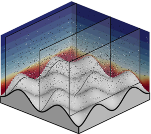Eight sets of particles ranging from $St^+ = 1$ to 1000 each with 200 000 particles, are randomly distributed in the core of the pipe $0 < r/R_0 < 0.55$ (see figure 1), and the initial velocity of the particles is set to be equal to the fluid's bulk velocity for faster particle statistics convergence. Eight particle diameters and four roughness heights provide us with $32$ cases to systematically study the effect of roughness induced turbulence on particles. The two-phase flow simulation is run for at least ${\rm \Delta} t^+ \approx 10\,800$ to reach a statistically steady state, independent of the initial conditions and particle statistics are averaged for at least ${\rm \Delta} t^+ > 720$. Table 1 shows the summary of the range of particles in the flow, whereas table 2 provides details of the rough-wall pipes.

Figure 1. Sketch of the computational domain of the rough-wall pipe with $h^+ = 20$ and the initial positions of the particles. The different colours illustrate the particles with different $St^+$ and only 10 000 particles are shown for clarity. The $x$-axis is in the streamwise direction and the radial distance, $r$, is measured from the centre of the pipe; $L_x$ is the length of the pipe. The plot shows the initial concentration of the particles (solid black line) and the injected velocity of the particles $u^{p+}$ (red dotted line) relative to the mean velocity profile of the fluid $U^+$ (red dashed line).

Table 1. Summary of the different particle types used in the simulation.

Table 2. Roughness characteristics and mean flow properties; $k_a^+$ and $k_{rms}^+$ are the average and root-mean-square roughness heights and $ES$ is the effective slope; ${\rm \Delta} U^+$ is the Hama roughness function and ${\rm \Delta} t^+$ is the viscous scaled time step.

3. Smooth vs rough wall

A visual comparison between the instantaneous distribution of particles with $St^+ = 1$ and $100$ for the unwrapped smooth- and rough-wall pipe ($h^+ =20$) is presented in figure 2. In figure 2(a), we observe that the particles with $St^+ = 1$ (in white) are randomly distributed throughout the domain whereas the heavy particles with $St ^ + = 100$ (in black) accumulate at the wall. The segregation between these two different particles is clearly illustrated in the streamwise–wall-normal slice in $(i)$. This phenomenon of particle migration to the smooth wall for inertial particles is due to turbophoresis (particle migration due to turbulence) and is well studied in the literature (e.g. Reeks Reference Reeks1983; Guha Reference Guha1997; Balachandar & Eaton Reference Balachandar and Eaton2010). On the other hand, for the rough-wall case, particles with $St^+ = 100$, which are inertial, collide and bounce off the wall and are homogeneously distributed throughout the pipe, as observed in the streamwise–wall-normal plane at different azimuthal slices (figure 2ii–$iv$).

Figure 2. Particle distribution of $St^+ = 1$ (in white) and $St^+ = 100$ (in black) for the (a) smooth-wall and (b) rough-wall cases with $h^+ = 20$ projected onto a flat plane. Coloured contour shows the time-averaged streamwise velocity. Streamwise–wall-normal slices corresponding to the $(i)$ smooth wall and the $(ii,iii,iv)$ rough wall at different spanwise locations which are locally smooth and rough. The black line in the roughness canopy show the region where $U^+ = 0$ and the black arrows show the accumulation of $St^+ = 1$ particles.

Figure 3 shows the plot of the normalised particle concentration $(C/C_0)$ against the viscous scaled wall-normal height comparing the (a) smooth-wall and (b) rough-wall cases, and also comparing the effects of different particle Stokes number (c) $St^+ = 1$ and (d) $St^+ = 100$; $C_0$ is the averaged particle concentration defined as the total number of particles with the same $St^+$ divided by the total volume of the pipe and $C$ is the local particle concentration (number of particles in an annular region divided by its volume). Figure 3(a) shows the smooth-wall case, where $C/C_0$ peaks at the wall, which is the usual case of particle migration due to turbophoresis. Not surprisingly, larger particles tend to migrate more towards the wall because once they are in the low-velocity region close to the wall, due to their large inertia it is difficult for them to leave the wall. As there are few particles in the centre of the pipe for $St^+ = 10$ and 100, the concentration profile is quite low (of $O(10^{-2})$) and therefore noisy.

Figure 3. Normalised particle concentration against viscous scaled wall-normal height for (a) smooth wall and (b) rough wall with $h^+ = 20$. Panels (c) and (d) show the concentration for particles with $St^+ = 1$ and $100$, respectively. Red arrows show the peaks in concentration in the roughness canopy. Sketches at the top illustrate the simulated pipes with different roughness heights.

Particles with very large $St^+$ (e.g. $St^+ = 1000$) are very sluggish due to the large particle relaxation time and, for the current range of simulation time, are still being transported to the wall.

For the rough-wall case (in figure 3b), spikes in concentration are observed for particles with $St^+ = 1$ and $10$ within the roughness canopy, as these light particles are trapped in the wake of the roughness and accumulate on the leeward side and at the trough of the roughness (see figure 2iii,$iv$). It is expected that as $t^+ \rightarrow \infty$, all of the light particles will accumulate in these regions. Interestingly, for small particles of $St^+=1$ (cf. figure 3c) no distinct spike in concentration is observed for the rough-wall case with $h^+ = 5$. This is due to the fact that the roughness is not steep enough to cause large flow separation events leeward of the roughness, and hence trap particles.

Inertial particles with large $St^+$ (cf. figure 3d), which would otherwise accumulate to the smooth wall, collide with the rough wall and are distributed throughout the pipe, and lead to $C/C_0 \approx 1$, consistent with the findings of Milici et al. (Reference Milici, De Marchis, Sardina and Napoli2014). This is also true for the rough-wall case with $h^+ = 5$ despite having a very small roughness height that would typically be considered as a hydrodynamically smooth surface (e.g. Jiménez Reference Jiménez2004).

Overall, it is apparent from figure 3 that particle concentration shows distinct features (for varying $St^+$ and $h^+$) within the roughness canopy and outside of it (the roughness sublayer). In the following two sections we focus on each of these regions.

4. Roughness canopy

The roughness canopy is the region occupied by the roughness $-h<y<h$ and for the smooth wall is defined as the viscous regime where $0<y^+<5$. This region is important in understanding the deposition mechanism of the particles where numerous experimental and theoretical works have been conducted for the past half a century to predict the deposition velocity and particle collection efficiency (e.g. Liu & Agarwal Reference Liu and Agarwal1974; Reeks & Skyrme Reference Reeks and Skyrme1976; Guha Reference Guha1997).

Most studies, however, have been focused on the smooth-wall flows. In the rough-wall case, the particle collection efficiency can be estimated by calculating the mean concentration in the roughness canopy. Figure 4(a) shows the contour of the normalised average concentration $\log (C/C_0)$ in the roughness sublayer plotted as a function of $h^+$ and $St^+$. The sketches in figure 4(i–$iv$) illustrate the different deposition and resuspension mechanism for smooth and rough walls at different $St^+$ and $h^+$ locations as indicated in figure 4(a).

Figure 4. Plot of the (a) contour of the concentration in the viscous/roughness canopy region and (b) the corresponding concentration trends. Sketches (i), (ii), (iii) and ($iv$) illustrate the distribution of particles along the streamwise–wall-normal plane. Particle trajectory close to the rough wall ($h^+ = 20$) for (c) $St^+ = 1$ and (d) $St^+ = 100$. The time interval between points is ${\rm \Delta} t^+ = 3.6$, thus, the spacing between points provides an indication of the velocity of the particles.

Consider the smooth-wall scenario in figure 4(a), i.e. $h^+=0$, and increasing $St^+$, i.e. going from (iii) to ($iv$) and depicted in the sketches in figure 4(iii,$iv$). A cut across this concentration plot is also shown in figure 4(b) with a black dashed line. The increasing particle concentration with increasing $St^+$ is readily evident, and, as mentioned before, is due to the turbophoretic effect. Next, we take $St^+=1$, and on 4(a) we move vertically from (iii) to (i). The corresponding schematics are in figure 4(i,iii). The particle concentration increases with increasing $h^+$, and this is simply the effect of particles with low inertia getting trapped in the recirculating region occurring behind the roughness ‘hills’ (see figure 4c). However, a slight decrease in concentration occurs at $h^+ = 5$ and this is because there are no recirculating regions due to the small roughness height. The increased velocity in the roughness canopy in fact reduces $C$ compared to the smooth-wall case.

Now, if we increase the $St^+$ to a $100$ and increase $h^+$ (i.e. from ($iv$) to (ii)) going vertically in figure 4(a), the concentration decreases. This illustrates the effect of turbophoresis, which tries to bring the particles to the wall, being counteracted by the increasing collision of the particles with the roughness elements that tries to reduce the concentration at the wall. Figure 4(d) shows the trajectory of particles with $St^+ = 100$ close to the roughness.

Finally, we see a minimum particle concentration at approximately $St^+\approx 50$ when we move horizontally at a fixed $h^+=20$. This is the location where the particle collision effect (hence reduction in $C$) overtakes the turbophoresis effect (of increasing $C$). Various cuts across figure 4(a) are shown as lines in figure 4(b). The varying trend of $C$ at different $h^+$ simply quantifies the effects described above.

Results from our regular three-dimensional roughness simulation may provide some insight into the transport and deposition of particles in irregular roughness (due to its practical importance), which contains regions which are locally more or less ‘rough’ (that could be measured by calculating the local effective slope or roughness parameter). At regions that are locally rough, there will be an increased tendency for particles with small $St^+$ to accumulate at the wake of roughness and regions of stagnant flow in the roughness canopy. For particles with larger $St^+$, the wall collision angle would be more acute and would result in more particles travelling against the mean flow as compared to a region which is locally less ‘rough’. Although our results provide some suggestions of behaviour over irregular roughness, a full effect requires further investigation.

5. Roughness sublayer

The roughness sublayer is the region where the influence of the roughness is felt by the fluid and causes the turbulent statistics for the rough wall to be different from the smooth-wall case. The thickness of the roughness sublayer for these sinusoidal roughnesses is found to scale with the roughness wavelength (Chan et al. Reference Chan, MacDonald, Chung, Hutchins and Ooi2018), and is defined as the region in the range $h<y<\lambda /2$. For the smooth wall, the buffer region is defined as the region in the range $5<y^+<50$.

Figure 5(a) shows the $\log (C/C_0)$ plot for the roughness sublayer in a manner similar to figure 4(a) for the roughness canopy. Figure 5 is, however, less dramatic, showing decreased regions of $C$ in the two regions (intermediate-$St^+$/small-$h^+$ and small-$St^+$/large-$h^+$), and this is because most particles have gone to the wall for these parameters. Nevertheless, the interesting feature of the roughness sublayer is that it is an ideal place to observe the effect of roughness generated turbulence on particle velocity and concentration statistics.

Figure 5. Plot of the (a) contour of the concentration in the buffer/roughness sublayer region and (b) the corresponding concentration trends.

In fact, the strong coherent sweep and ejection events by the fluid inside the roughness sublayer play an important part in the transfer mechanism of particles, as suggested by Marchioli & Soldati (Reference Marchioli and Soldati2002). They described the transport mechanism of particles in a smooth wall and found that the particle deposition is due to particles accumulating into specific regions in the buffer layer where the coherent structures reside. For a turbulent rough-wall flow, these structures in the roughness sublayer have been modulated by the roughness and the wall effects play an important role.

To understand the dynamics of the particles in the roughness sublayer (or the equivalent buffer region of the smooth wall), the wall-normal velocity of the particles $-u_r^p$ (since this velocity component takes particles towards/away from the wall) is compared with the local fluid velocity sampled by the particle. The momentum transfer of fluid is quantified by the Reynolds stress $- u^{\prime }_{x} u_{r}^{\prime + }$, whereas, following Soldati & Marchioli (Reference Soldati and Marchioli2009), we consider $- |u^{\prime }_{x} |u_{r}^{\prime + }$, where positive values are associated with coherent ejections and negative values are associated with coherent sweeps. Figure 6 shows the joint probability density function (PDF) of $-u_r^p$ against $- |u^{\prime }_{x} |u_{r}^{\prime + }$.

Figure 6. Joint PDF of particle wall-normal velocity and coherent fluid events for (a) $St^+ = 1$, (b) $St^+ = 50$ and (c) $St^+ = 1000$ for the smooth wall and rough wall with $h^+ =20$.

Although the turbulent structures for the rough-wall cases differ from the smooth wall, figure 6(a) for $St^+=1$ is similar because particles are driven towards the wall by sweeping events and are transported away from the wall by ejection events. Probability of these events occurring is presented in table 3. While low $St^+$ particles act as flow tracers, high $St^+$ particles filter most of the spectrum of turbulent eddies, such that they are unresponsive to the coherent structures. This is observed in figure 6(c) where smooth wall with $St^+ = 1000$ has a smaller range of $-u_r^p$ compared to $St^+ = 1$, although the transport mechanism is still influenced by the sweep and ejection events with probabilities of 55.4 % and 56.8 %, respectively, that are slightly above 50 %. The values of $P \approx 56\,\%$ for sweeps/ejections for $St^+ = 1000$ should be compared to the $P \approx 95\,\%$ for $St^+ = 1$ that is dominated by sweep/ejection events. For $St^+ = 1000$, in comparison with the smooth-wall case, for the rough-wall case in figure 6(c), a large scatter in $-u_r^p$ and $- |u^{\prime }_{x} |u_{r}^{\prime + }$ is observed with the particles’ wall-normal velocity being uncorrelated with the sampling of sweep and ejection events ($P \approx 50\,\%$). Wall collision is the dominant mechanism, which has no directional preference, and this results in a virtually identical probability of sampling in all four quadrants.

Table 3. Probabilities conditioned on positive or negative particle wall-normal velocity $-u_r^p$ and sweep ($- |u^{\prime }_{x} |u_{r}^{\prime + }<0$) or ejection events ($- |u^{\prime }_{x} |u_{r}^{\prime + }>0$) in the buffer/roughness sublayer region. The probabilities are defined as $P_I = P(- |u^{\prime }_{x} |u_{r}^{\prime + } > 0$ and $-u_r^p > 0 )$, $P_{II} = P(- |u^{\prime }_{x} |u_{r}^{\prime + } < 0$ and $-u_r^p > 0 )$, $P_{III} = P(- |u^{\prime }_{x} |u_{r}^{\prime + } < 0$ and $-u_r^p < 0 )$, $P_{IV} = P(- |u^{\prime }_{x} |u_{r}^{\prime + } > 0$ and $-u_r^p < 0 )$. Probabilities for the smooth-wall case with $St^+=50$ were evaluated at time interval of $3600<{\rm \Delta} t^+<5400$ ($20<U_\tau {\rm \Delta} t/R<30$).

Particles in the intermediate Stokes number are found to be most affected by the dynamics of the buffer region in a smooth-wall pipe (e.g. Picano et al. Reference Picano, Sardina and Casciola2009). In the rough-wall pipe, large positive values of $-u_r^p$ are observed in figure 6(b) for particles with $St^+ = 50$ due to collision with the wall. The negative $-u_r^p$ region on the other hand has similar trends with $St^+ =1$ particles, albeit with an increased probability for positive $- |u^{\prime }_{x} |u_{r}^{\prime + }$ (ejection) events. At intermediate $St^+$, these particles are influenced both by the turbulent flow and the wall collisions. The particles with $St^+=50$ in the smooth-wall case have all migrated to the wall at this time (${\rm \Delta} t^+ = 10\,800$). Therefore, the statistics for this particular $St$ are evaluated at an earlier time ($3600<{\rm \Delta} t^+<5400$), where the particles are still fleeing the centre towards the wall of the pipe.

Another statistic to consider when analysing the roughness sublayer is the probability density function of the streamwise and wall-normal velocities of both the fluid and the particles. Figure 7 shows the probability distributions of the streamwise and radial velocities normalised by the bulk velocity in the roughness sublayer for all rough and smooth cases.

Figure 7. Probability density function of the axial (a,c,e) and wall-normal (b,d,f) velocity normalised by the bulk velocity for $St^+ = (a,b)$ 1, $(\textit {c},\textit {d})$ 50 and $(\textit {e},\textit {f})$ 1000 in the roughness sublayer/buffer layer. The dashed line shows the probability density function of the sampled fluid velocity.

For particles with a very small Stokes number ($St^+ = 1$ in figure 7a,b), as one would expect, the $P(u_x/U_b)$ and $P(-u_r/U_b)$ profiles (in dark solid lines) of the particles are similar to the fluid probabilities (in light dashed lines). When the $St^+$ increases to $50$, the probability of the wall-normal velocity (figure 7d) is asymmetric as the collision with the rough wall causes particles to bounce away from the wall (i.e. a negative tail), and this effect increases with increasing $h^+$. After colliding with the wall, the particles become entrained by the bulk flow and only subtle differences between the fluid and particle streamwise velocity probabilities are observed in figure 7(c). In this $St^+$ regime, the particles are not only driven by the turbulent structures of the rough wall but also effected by the wall collision. While the work of Milici et al. (Reference Milici, De Marchis, Sardina and Napoli2014) concluded that the particle deposition mechanisms between smooth and rough walls are driven by the different turbulent structures, we would argue that the wall collision is also a prominent mechanism for particles with $St^+ = 50$ and higher.

Sluggish, heavy particles with a large Stokes number in figure 7(f) on the other hand collide with the rough wall and bounce towards the opposite wall while retaining their inertia to form a symmetric $P(-u_r/U_b)$ profile. As the height of the roughness increases, the steepness of the roughness measured by its ‘effective slope’ (e.g. Napoli, Armenio & De Marchis Reference Napoli, Armenio and De Marchis2008), increases. The collision angle becomes more acute and the tendency for the particle trajectory to be in the opposite direction to the mean flow increases with $h^+$, as observed in the leftward shift of the $P(u_x/U_b)$ profiles in figure 7(e).

To reemphasise the above point of particle collision with increasing $St^+$, we visualise the transport of the particles in different regimes. Five sample particles with $St^+ = 1,50$ and 1000 in the rough-wall case $h^+ = 20$ are tracked and plotted in figure 8. Only two of the five particles tracks are observed for $St^+ = 1$ (figure 8a) as three of the particles are trapped in the roughness canopy. Comparing $St^ + = 50$ particles with $St^+ = 1$ particles, the pathlines of the heavier particles are more aligned with the mean flow and are less affected by the sudden turbulent changes in the flow. Collision angle for particles with $St^ + =50$ is quite shallow compared to $St^+ = 1000$ and the particles are entrained by the bulk flow after bouncing off the wall. Due to the large inertia of particles with $St^+ = 1000$, the trajectories of the particles are almost independent of the flow, and are greatly affected by the roughness topography. The transverse dispersion of the particles and enhanced wall collision frequency due to roughness observed by Kussin & Sommerfeld (Reference Kussin and Sommerfeld2002) in their experimental work are consistent with our observation. Current simulations have been conducted at a relatively low Reynolds number where there is limited scale separation between the small and large scale structures. At higher Reynolds number, the interactions between the large scale motions and the near-wall small scale structures may affect the transport and deposition mechanism of particles in the smooth-wall pipe, but this remain to be seen.

Figure 8. Particle tracks for 5 particles with (a) $St^+ = 1$, (b) 50 and (c) 1000 in the rough-wall pipe with $h^ + = 20$. The larger black circle symbol denotes the start of the tracking and particles are shaded from light to dark as a function of the radial location. The time interval between points is ${\rm \Delta} t^+ = 3.6$, thus, the spacing between points provides an indication of the velocity of the particles.

Having looked at both the roughness canopy and roughness sublayer, in the final part of the results, we now compare the average particle speed within the whole pipe and compare it to the bulk fluid velocities.

6. Average particle motion

The averaged particle velocity in the streamwise direction, $u^p_b = \sum _{i=1}^{N_p} u_{x,i}^p/N_p$ normalised by the fluid bulk velocity, $U_b$ is plotted in figure 9 to quantify the transport of particles in pipes with different roughness heights. This parameter is similar to the particle bulk Reynolds number $Re^p_b = u^p_b \delta /\nu$ which was introduced by Milici et al. (Reference Milici, De Marchis, Sardina and Napoli2014) but also takes into account the different bulk flow rate of the fluid which decreases with increasing roughness height at a fixed friction Reynolds number.

Figure 9. Average particle streamwise velocity normalised by the bulk velocity $u^p_b/U_b$ against $St^+$ for the smooth and rough cases showing the $(I)$ flow influenced, $(II)$ flow and wall influenced and $(III)$ wall influenced regions. Particles of the smooth-wall case with $St^+ > 100$ have not fully converged and are expected $u_b^p \rightarrow 0$ as $t\rightarrow \infty$. The smaller circular grey symbols are the instantaneous bulk velocities with increasing size corresponding to increased simulation time of ${\rm \Delta} t^+ =$ 9000, 10 800, 12 600.

For convenience, we divide the figure into three regimes; $St^+ =1$ to $10$, $10$ to $100$ and $100$ to $1000$. For low $St^+$ cases (regime $I$), particles in the smooth-wall case have a velocity similar to the fluid. This is of course due to the particles following the fluid almost faithfully. With increasing $h^+$, $u^p_b$ decreases because more and more light particles get trapped in the roughness canopy where they have reduced velocities. For larger $St^+$ (regime $II$), the $u^p_b$ for the smooth-wall case drops precipitously due to turbophoresis, which gathers particles at the wall, and where the velocity is close to zero. For rough-wall cases with higher $St^+$, the trend is opposite, where increasing collisions take the particles way from the wall into the pipe flow region where velocities are higher. For current regular three-dimensional sinusoidal roughness, $u^p_b$ reaches up to $20\,\%$ higher than the bulk velocity for case $h^+ = 20$. Interestingly, when $St^+ = 100$, the particles travel on average at a similar velocity as the bulk velocity $u^p_b/U_b \approx 1.07$ for all of the rough cases. With further increase in $St^+$ (i.e. in regime $III$), $u^p_b$ for all roughness cases reduces. As mentioned before, the effect of turbophoresis becomes important with increasing $St^+$ and to some extent reduced the particles being taken into the bulk of the pipe, and this in turn brings $u^p_b$ down.

Notice that in figure 9 we include data from the irregular two-dimensional roughness of Milici et al. (Reference Milici, De Marchis, Sardina and Napoli2014) which also peak in regime $II$. By only looking at the data of Milici et al. (Reference Milici, De Marchis, Sardina and Napoli2014) one might incorrectly surmise that $u^p_b/U_b$ would asymptote to a constant, and now we see that this need not be the case. The trends for $u^p_b/U_b$ are somewhat roughness topography dependent and the differences between Milici et al. (Reference Milici, De Marchis, Sardina and Napoli2014) and the current data could also be due to the different flow geometry (pipe vs channel), but it is expected that $u^p_b/U_b$ decreases at the limit $St^+ \rightarrow \infty$. This might not be the case if the gravitational force is included, where it is important for particles with large $St^+$; $u^p_b$ for the smooth-wall flow appears to increase when $St^+ > 100$ but it is because the sluggish particles are still in the core of the pipe and require more time to be transported to the wall (simulation needs to be run for an order of magnitude longer).

Although we can describe the different changes to $u^p_b/U_b$ in figure 9, the situation is not completely satisfactory from a scaling point of view. That is, the different curves for different $h^+$ seem to peak at different $St^+$, and one might wonder if the abscissa could be scaled differently (to $St^+=\tau _p/\tau _f$) to collapse the data and hence reveal a common underlying mechanism. In fact, we know that viscous effects (taken into account by $\tau _f$) have very little to do with the $u^p_b/U_b$ distribution for roughness cases. Indeed, in plotting figure 9 we neglected any roughness time scale that might play a role. Our roughness has two characteristic length scales, the wavelength $\lambda$ and roughness height ($h$). So, apart from the time scales of particles ($\tau _p$) and the viscous effect ($\tau _f$) we introduce a roughness time scale, which could be $\lambda /U_\tau$ or $h/U_\tau$ or $(\lambda /h)(\lambda /U_\tau )$. Now, it turns out that if we defined the roughness time scale $\tau _r = (\lambda /h)(\lambda /U_\tau )$, and a Stokes number based on roughness as the particle relaxation time normalised by the roughness time scale $St_r = \tau _p/\tau _r$, the data seem to collapse. Our data of $u^p_b/U_b$ from figure 9 are re-plotted in figure 10 against $St_r$. This suggests, at least empirically, that both $\lambda$ and $h$ have an effect on collisions, and hence on $u^p_b/U_b$. It remains to be seen how $u^p_b/U_b$ changes by varying $\lambda$, which is fixed for the present study.

Figure 10. Average particle streamwise velocity normalised by the bulk velocity $u^{p}_{b}/U_b$ against Stokes roughness number $St_r = \tau _p/\tau _r$ for the smooth and rough cases.

7. Summary and conclusions

A DNS of two-phase flow has been conducted in a turbulent rough-wall pipe with sinusoidal roughness for a range of $St^+$ and $h^+$. The transport and deposition mechanisms of the particles in a turbulent rough-wall flow are dependent on the $St^+$ of the particles and also on some measure of the roughness, which we have chosen to be the roughness height $h^+$. Three regimes are observed and are elaborated below:

1. (I) Low $St^+$: particles with low Stokes numbers (approximately below $St^+ =10$) behave like tracers and follow the path of the fluid. For very small roughness heights $h^+ = 5$, the flow characteristics of the rough wall are similar to those of the smooth wall and therefore the particle statistics, such as the near-wall concentration, are very similar between the rough and smooth cases. As the roughness becomes more pronounced, changes in the near-wall flow cause these particles to be trapped in the stagnant flow in the trough of the roughness and at the leeward side of the rougness where the flow separates.

2. (II) Medium $St^+$: at intermediate Stokes numbers (approximately $10<St^+<100$), the transport mechanism of the particles is balanced by both the turbulent structures of the flow and also collisions with the rough wall. Inertial particles have the tendency to be attracted towards the wall due to turbophoresis. In a turbulent rough-wall flow, the near-wall concentration of particles decreases as the particles are no longer trapped in the roughness canopy but rather collide and bounce off the rough wall. In the roughness sublayer, the particles possess large positive wall-normal velocities due to wall collisionsbut have similar streamwise velocities as the fluid.

3. (III) High $St^+$: particles with large Stokes numbers (approximately $St^+>100$) are sluggish and the inherent inertia of the particles means that their trajectory is unresponsive to the short time scales of the turbulent flow. The larger the particles’ $St^+$, the larger the turbophoretic effect on the particles, causing a higher frequency of particle collisions with the rough wall. The topography of the roughness becomes important in determining the trajectory and dispersion of the particles as the particle collision angle becomes more acute with increasing roughness slope.

It is important to recall that these results are limited to heavy particles which are small compared to the smallest turbulent scales in the flow and much denser than the carrier phase. In addition, the work here assumes a dilute discrete phase where particle–particle interactions and the back force from the particles on the fluid are not accounted for. A previous study by De Marchis & Milici (Reference De Marchis and Milici2016) has found a decrease in the particle velocity fluctuations when conducting two-way coupling simulations and this could be important for the rough-wall case. These additional parameters would have to be investigated separately in future works.