INTRODUCTION
The Chronos 14Carbon-Cycle Facility (henceforth Chronos) is a new dedicated radiocarbon (14C) and stable isotope facility established at the University of New South Wales, Sydney (UNSW), in collaboration with the Australian Nuclear Science and Technology Organisation (ANSTO). UNSW had previously been home to a radiocarbon laboratory in the School of Chemistry (spanning 1960s to 1986) (Southwell-Keely Reference Southwell-Keely2020), but Chronos has been established as a cross-faculty facility housed in a new laboratory space within the Science and Engineering Building, as part of the Mark Wainwright Analytical Centre (MWAC). Funded through the UNSW 2025 Strategic Plan, the aim of this facility is to provide greater radiocarbon research capacity for the Earth, Environmental and Archaeological sciences.
As the planet faces unprecedented rates of global environmental and societal change in the Anthropocene, there is an urgent need to improve our understanding of the Earth System (Lewis and Maslin Reference Lewis and Maslin2015; Steffen et al. Reference Steffen, Broadgate, Deutsch, Gaffney and Ludwig2015, Reference Steffen, Rockström, Richardson, Lenton, Folke, Liverman, Summerhayes, Barnosky, Cornell and Crucifix2018). A key source of uncertainty over the timing and impacts of future change is that historical (instrumental) records of change are too short (since CE 1800) and their amplitude too small relative to projections for the next century (IPCC 2018), raising concerns over our ability to successfully plan for future change. Growing populations threaten to erode the sustainable use of the global resource base, including water resources, with substantial economic implications. In Australia alone, groundwater supplies support manufacturing, agriculture, and mining worth $34 billion/year, but are facing increasing exploitation (Deloitte Access Economics 2013). Future climate extremes are likely to increase in amplitude and frequency compared to the historic period, enhanced by climate-human-carbon feedbacks (Friedlingstein et al. Reference Friedlingstein, Meinshausen, Arora, Jones, Anav, Liddicoat and Knutti2013; Le Quéré et al. Reference Le Quéré, Andres, Boden, Conway, Houghton, House, Marland, Peters, van der Werf and Ahlström2013; Bradford et al. Reference Bradford, Wieder, Bonan, Fierer, Raymond and Crowther2016; Graham et al. Reference Graham, Baker and Andersen2015; Randerson et al. Reference Randerson, Lindsay, Munoz, Fu, Moore, Hoffman, Mahowald and Doney2015; Fu et al. Reference Fu, Gasser, Li, Tao, Ciais, Piao, Balkanski, Li, Yin and Han2020; McDonough et al. Reference McDonough, Santos, Andersen, O’Carroll, Rutlidge, Meredith, Oudone, Bridgeman, Gooddy and Sorensen2020). Such changes could have substantial and irreversible consequences for Australia’s (and the world’s) climate and environment.
Detailed radiocarbon analyses of Earth, environmental, and archaeological records have considerable potential for providing insights into the mechanisms and impacts of regional and global change that pre-date the observational period (Thomas Reference Thomas2016; Dougherty et al. Reference Dougherty, Thomas, Fogwill, Hogg, Palmer, Rainsley, Williams, Ulm, Rogers and Jones2019; Reimer et al. Reference Reimer, Austin, Bard, Bayliss, Blackwell, Bronk Ramsey, Butzin, Cheng, Edwards and Friedrich2020; Rockman and Hritz Reference Rockman and Hritz2020; Steffen et al. Reference Steffen, Richardson, Rockström, Schellnhuber, Dube, Dutreuil, Lenton and Lubchenco2020). A wealth of “natural archives” (or “palaeo archives,” such as tree rings, lake sediments, speleothems, and ice cores) are available to extend instrumental records of environmental change. In combination with increasingly detailed archaeological analyses, records of past change offer an improved understanding of environmental variability and impacts in the Earth system but require the development of accurate age models for precise comparison. For instance, past extreme and rapid climate changes are now widely recognized in numerous natural archives and appear to be associated with substantial disruptions in the global carbon cycle (Treble et al. Reference Treble, Baker, Ayliffe, Cohen, Hellstrom, Gagan, Frisia, Drysdale, Griffiths and Borsato2017; Steffen et al. Reference Steffen, Rockström, Richardson, Lenton, Folke, Liverman, Summerhayes, Barnosky, Cornell and Crucifix2018; Fogwill et al. Reference Fogwill, Turney, Menviel, Baker, Weber, Ellis, Thomas, Golledge, Etheridge and Rubino2020). These major environmental changes are often paralleled by patterns of past human migration and adaptation (Turney and Hobbs Reference Turney and Hobbs2006; Zhang et al. Reference Zhang, Lee, Wang, Li, Pei, Zhang and An2011; O’Connell et al. Reference O’Connell, Allen, Williams, Williams, Turney, Spooner, Kamminga, Brown and Cooper2018; Becerra-Valdivia and Higham Reference Becerra-Valdivia and Higham2020; Douglass and Cooper Reference Douglass and Cooper2020).
To better understand contemporary processes in the Earth system, there is an increased demand for a wide range of radiocarbon applications. An expanded network of annually-resolved tree-ring records in regions where there is currently a dearth of datasets (e.g., the tropics and subantarctics) (Brienen et al. Reference Brienen, Schöngart and Zuidema2016; Haines et al. Reference Haines, Gadd, Palmer, Olley, Hua and Heijnis2018; Hogg et al. Reference Hogg, Heaton, Hua, Palmer, Turney, Southon, Bayliss, Blackwell, Boswijk and Bronk Ramsey2020) offers the opportunity to reduce the uncertainty surrounding contemporary and projected multidecadal to subannual carbon-climate dynamics (Friedlingstein et al. Reference Friedlingstein, Jones, O’Sullivan, Andrew, Hauck, Peters, Peters, Pongratz, Sitch and Le Quéré2019; Varney et al. Reference Varney, Chadburn, Friedlingstein, Burke, Koven, Hugelius and Cox2020). In the subsurface, radiocarbon can provide insights into the sources and sinks of organic carbon in drinking water treatment (Bridgeman et al. Reference Bridgeman, Gulliver, Roe and Baker2014), understanding the source of river evaded carbon dioxide (Billett et al. Reference Billett, Garnett and Harvey2007), and determining the age and source of labile aquatic organic matter in natural and urban systems (Hedges et al. Reference Hedges, Ertel, Quay, Grootes, Richey, Devol, Farwell, Schmidt and Salati1986; McDonough et al. Reference McDonough, Santos, Andersen, O’Carroll, Rutlidge, Meredith, Oudone, Bridgeman, Gooddy and Sorensen2020). Along with partners ANSTO, the new facility enhances capacity for these analyses and aims to address these global questions by increasing the number of 14C measurements available to the scientific community. This was the primary motivation for the establishment of the Chronos facility.
INSTRUMENTS
The centrepiece of the Chronos facility is a 200 kV MIni-CArbon DAting System (MICADAS) Accelerator Mass Spectrometer. The first prototype of MICADAS was developed in 2007 integrating a unique low energy (200 kV), vacuum insulated acceleration unit at the Laboratory of Ion Beam Physics, ETH, Zurich (Synal et al. Reference Synal, Stocker and Suter2007; Wacker et al. Reference Wacker, Bonani, Friedrich, Hajdas, Kromer, Němec, Ruff, Suter, Synal and Vockenhuber2010a), and subsequently built and distributed by Ionplus. The MICADAS systems are now found in numerous institutions around the world (Kromer et al. Reference Kromer, Lindauer, Synal and Wacker2013; Bard et al. Reference Bard, Tuna, Fagault, Bonvalot, Wacker, Fahrni and Synal2015; Knowles et al. Reference Knowles, Monaghan and Evershed2019). In October 2019, a MICADAS was installed in the Chronos Facility. This is the 25th system in operation and the first to be located in the Southern Hemisphere. Chronos also includes a gas interface system for the direct injection of CO2 into the MICADAS (Gas Interface System or “GIS,” Ionplus) (Wacker et al. Reference Wacker, Fahrni, Hajdas, Molnar, Synal, Szidat and Zhang2013a), a cracker for gas samples sealed in glass tubes (Tube Sealing Equipment or “TSE,” Ionplus), three Elementar vario ISOTOPE cube elemental analyzers (EA) for sample combustion, an automated system to handle carbonates using wet chemistry (Carbonate Handling System 2 or “CHS2,” Ionplus), an automated graphitization system (Automated Graphitization Equipment 3 or “AGE3,” Ionplus), and an EA-coupled Elementar precisION® isotope ratio mass spectrometer (IRMS) (Figure 1).
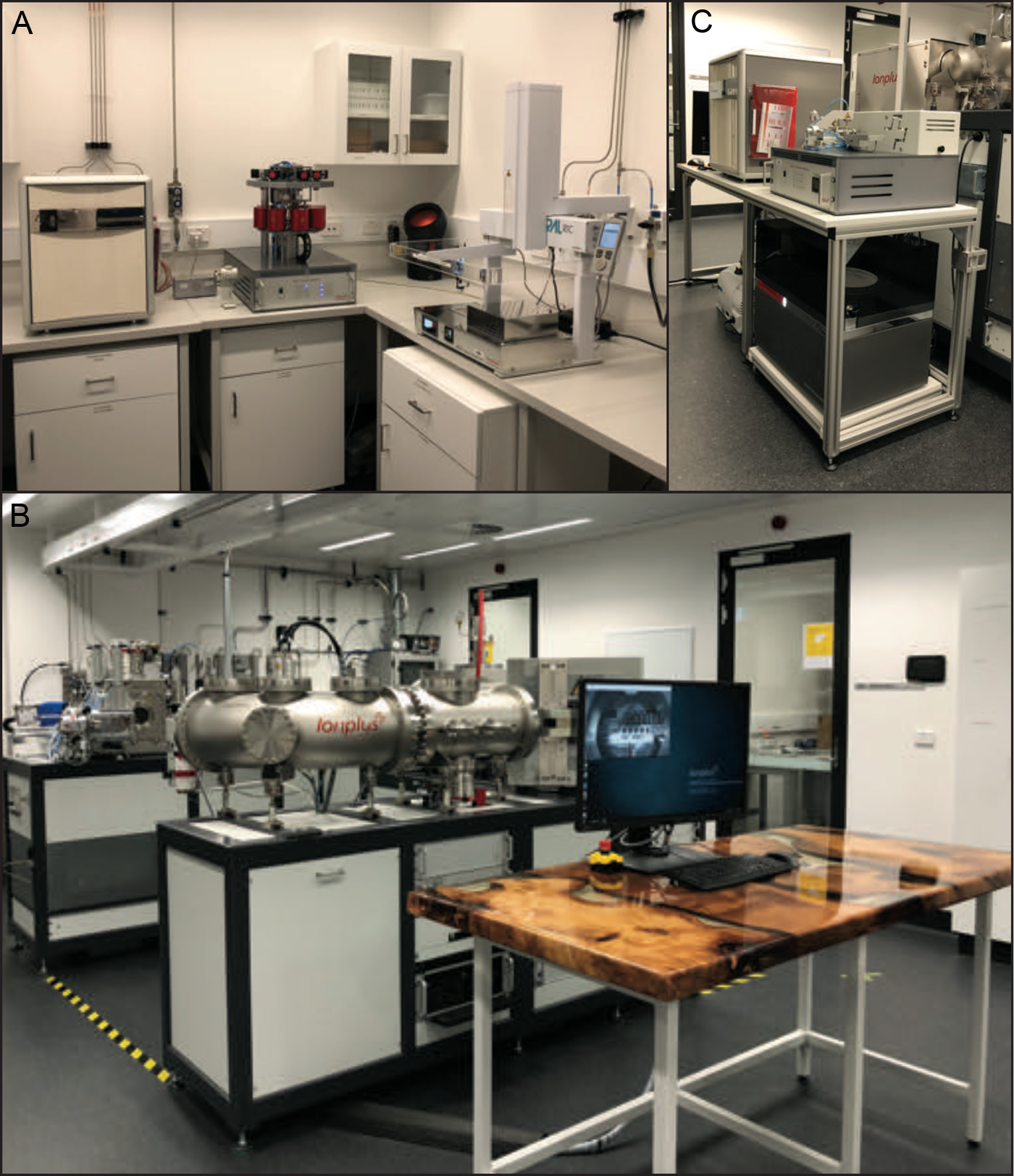
Figure 1 The Chronos 14Carbon-Cycle Facility at the University of New South Wales. Panel A: Elemental analyzer with Carbonate Handling System 2 and Automated Graphitisation Equipment 3. Panel B: The MIni-CArbon DAting System (MICADAS) with New Zealand ancient kauri workstation at the University of New South Wales. Panel C: Elemental analyzer coupled to an isotope ratio mass spectrometer with the Gas Interface System.
SAMPLE PREPARATION METHODS
The Chronos Facility is capable of handling a wide range of sample material types. Here we outline the sample preparation methods of the material types that have formed the focus for the facility during the first year of operation: wood, bone, carbonates, charcoal, peat, and pollen. The following describes the rational for selecting suitable samples for 14C analysis and subsequent processing at the Chronos facility.
Sampling
For bone and shell samples, where possible, the surfaces are cleaned by air abrasion with aluminium oxide powder to remove superficial contaminants. Bone fragments are then cut manually or using a small diamond disc, and both bone and carbonate (shell) samples are crushed with a pestle and mortar (stainless steel) prior to processing. For bone collagen pre-screening (see section below), sampling is undertaken by drilling with a cleaned tungsten carbide spherical burr drill bit. Here we follow DeNiro and Weiner (Reference DeNiro and Weiner1988) in their use of the term “collagen.”
For peat and lake sediments, terrestrial macrofossils are generally considered to be the most reliable material for 14C sample selection within a sediment matrix (Lowe and Walker Reference Lowe and Walker2000; Bronk Ramsey et al. Reference Bronk Ramsey, Staff, Bryant, Brock, Kitagawa, van der Plicht, Schlolaut, Marshall, Brauer and Lamb2012; Thomas et al. Reference Thomas, Turney, Hogg, Williams and Fogwill2019). Terrestrial macrofossils are carefully selected with tweezers and cleaned of surrounding sediment (under a low-power microscope if necessary). Fruits, leaves, stems, twigs, and branches are all suitable material, with dry weights of >3 mg. It is vital that roots or rootlets are removed to prevent contamination through the intrusion of younger carbon from overlying sediments. If terrestrial macrofossils cannot be identified, the humin or humic fraction from bulk peat/sediment samples is measured instead, though these fractions may be more vulnerable to contamination (Walker et al. Reference Walker, Lowe, Blockley, Bryant, Coombes, Davies, Hardiman, Turney and Watson2012; Strunk et al. Reference Strunk, Olsen, Sanei, Rudra and Larsen2020). If bulk peat/sediment is analyzed, care is taken to remove any roots prior to chemical pretreatment. If bulk sediment is not desirable or considered appropriate for a sequence, terrestrial microfossils, such as pollen, are targeted for dating (Brown et al. Reference Brown, Farwell, Grootes and Schmidt1992; Vandergoes and Prior Reference Vandergoes and Prior2003; Howarth et al. Reference Howarth, Fitzsimons, Jacobsen, Vandergoes and Norris2013; Tennant et al. Reference Tennant, Jones, Brock, Cook, Turney, Love and Lee2013). Pollen concentrates are extracted from bulk peat/sediment samples using modified palynological methodologies (Bennett and Willis Reference Bennett and Willis2002). If the pollen concentrations of bulk sediment samples are unknown, preliminary sample processing is performed to determine the sample quantity required (see below).
For tree rings, if tree cores are glued to core mounts, the wood is removed using a scalpel and then placed in acetone for 1–2 hr so that the glue becomes malleable and can be wiped from the core. Should any glue remain after this, a scalpel is used to cut the remaining glue from the core. Once a wood sample is dry, one of two methods is employed. For annual 14C measurement of tree rings, each ring is carefully cut from the sample using a scalpel. Care is taken to ensure that the sample does not extend beyond the selected ring boundaries. The annual ring is then cut into small, thin rectangular pieces (“matchsticks”) being certain that each piece spans the entire year’s growth (>10 mg although 50 mg is desirable depending on the age and condition of the sample). For multi-year dating (e.g., decadal-block samples), the ring boundaries bracketing the desired period are carefully sampled to make sure no growth extends beyond these rings.
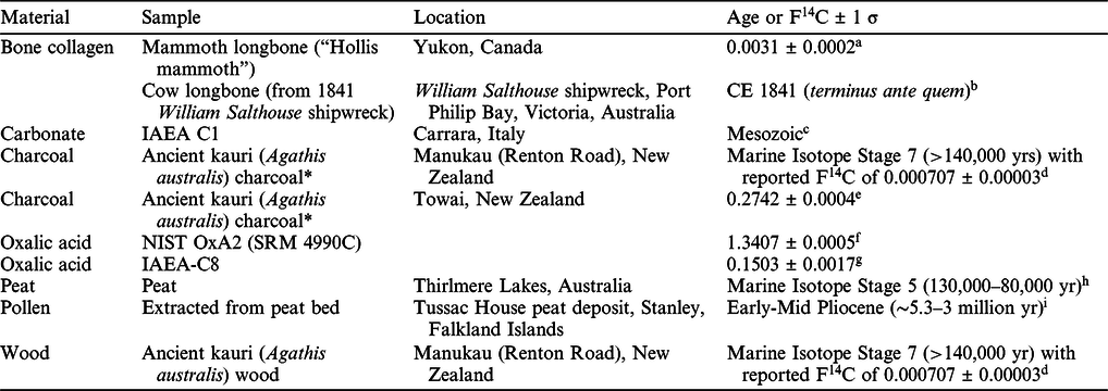
Chemical Pretreatment
Routine pretreatment methods at Chronos are identified with unique pretreatment (P) codes. These differ according to each material type, the sources of contamination, the degree of preservation, and are assigned following due assessment. If solvent is used to remove contaminants (e.g., glue on bone or wood) prior to pretreatment, the code is followed by an asterisk (e.g., UFC* or BABAB*). Samples are pretreated in batches of 16–28, depending on the material type. With every batch, we undertake at least one duplicate sample that undergoes separate chemical pretreatment for further quality control. Matrix-matched, known-age samples are included in each chemical pretreatment batch for background subtraction calculations and/or as quality assurance checks (Table 1). Following pretreatment, all samples are lyophilized (AdVantage Pro XL, SP Scientific). Glassware and equipment within Chronos are solely dedicated to radiocarbon dating. Prior to use, glassware is washed and baked in a 500ºC oven for 3 hr to reduce carbon contamination.
Table 1 Known-age and background samples used at the Chronos facility.
* These wood samples were charred inside a sealed stainless-steel pyrolysis vessel at 450ºC for 4 hr (following drying at 150ºC for 1 hr). The pyrolysis vessel had been previously baked at 600ºC for 1 hr.
a De La Torre et al. (Reference De La Torre, Reyes, Zazula, Froese, Jensen and Southon2019).
b Staniforth (Reference Staniforth1997).
c Dean (Reference Dean, Herz and Waelkens1988); Rozanski (Reference Rozanski1991).
d Hogg et al. (Reference Hogg, Fifield, Turney, Palmer, Galbraith and Baillie2006); Marra et al. (Reference Marra, Alloway and Newnham2006).
e Hogg et al. (Reference Hogg, Southon, Turney, Palmer, Bronk Ramsey, Fenwick, Boswijk, Friedrich, Helle and Hughen2016a, Reference Hogg, Southon, Turney, Palmer, Ramsey, Fenwick, Boswijk, Büntgen, Friedrich and Helle2016b).
f F14C value normalized to δ13C value of –25‰ (Rasberry Reference Rasberry1999; Bard et al. Reference Bard, Tuna, Fagault, Bonvalot, Wacker, Fahrni and Synal2015).
g Le Clercq et al. (Reference Le Clercq, Van Der Plicht and Gröning1997).
h Forbes et al. (Reference Forbes, Cohen, Jacobs, Marx, Barber, Dodson, Zamora, Cadd, Francke and Constantine2021).
i Unpublished site but preliminary work suggests correlation to Forest Bed at West Point, Falkland Islands (Macphail and Cantrill Reference Macphail and Cantrill2006).
Bone
To assess bone collagen preservation, samples might be first pre-screened for nitrogen content following Brock et al. (Reference Brock, Higham, Ditchfield and Bronk Ramsey2010a). Nitrogen content is a suitable proxy for collagen preservation as it derives exclusively from the protein component in bone (Sillen and Parkington Reference Sillen and Parkington1996). This method involves measuring the weight % N of 1 mg of whole bone powder with a CN elemental analyzer (vario ISOTOPE select, Elementar). Acetanilide (Sigma-Aldrich) is used as a standard.
For bone samples with conservation-derived contamination, solvent extraction precedes routine pretreatment. If the contaminant is known, e.g., shellac, tailored protocols following Brock et al. (Reference Brock, Dee, Hughes, Snoeck, Staff and Ramsey2018) are employed. Otherwise, samples are sequentially washed with acetone (30–60 min, 40ºC), methanol (30–60 min, 40ºC), and chloroform (30–60 min, at room temperature or “RT”) (Brock et al. Reference Brock, Higham and Ramsey2010b) and left to dry.
Routine pretreatment involves acid-base-acid (ABA) immersions, gelatinization (Longin Reference Longin1971), filtration, and ultrafiltration (Brown et al. Reference Brown, Nelson, Vogel and Southon1988) (pretreatment code “UFC”). If the sample is believed or shown to be poorly preserved, however, ultrafiltration is omitted (pretreatment code “SFC”). Depending on the bone sample and its degree of contamination, a SFC date should only be viewed as a terminus ante quem.
Sequentially, bone samples are placed in 0.5 M hydrochloric acid (3-4 rinses every 2 hr and overnight for approximately 20 hr; RT), 0.1 M sodium hydroxide (30 min; RT), and 0.5 M hydrochloric acid (1 hr; RT), with 3 rinses of Milli-Q® water between each reagent. Separation is either through decanting or glass pipetting (these are baked for 3 hr at 500ºC prior to use) and is typically aided by centrifugation. The crude collagen is then gelatinized in pH 3 solution at 75ºC for 20 hr, and the resulting gelatin is filtered using non-sterile syringe filters (Millex, Durapore®; 45 µm pore size). These are cleaned by flushing with 10 mL of Milli-Q® water, followed by 10 mL of 0.5 M HCl, and finally once more with 10 mL of Milli-Q® water. The syringe-filtered gelatin is then decanted into an ultrafilter (Sartorius™ Vivaspin™ Turbo 15, 30 kD MWCO, polyethersulfone membrane) and centrifuged at 2550 rpm until 0.5–1.0 mL of the >30 kD fraction remains. Ultrafilters are cleaned using Milli-Q® water by rinsing, centrifuging at 2550 rpm for 10 min twice, ultrasonication for 1 hr, soaking overnight, a further three centrifugations, and a final rinse. After the fourth centrifugation, a sample of the Milli-Q® water in the ultrafilter is collected and tested for wt% C as a quality control using an EA. Finally, the ultrafiltered gelatin is transferred into a test tube using clean glass pipettes to be lyophilized.
Carbonates
If carbonate samples are too fragile for shot blasting, these are placed inside exetainers (Exetainer®, Labco) and depending on the sample size, leached using the necessary amount of 0.1 M HCl to remove secondary carbonates in the outer layer (10–20% for foraminifera and coral, and 40–50% for shell; pretreatment code “LC”) (Wacker et al. Reference Wacker, Fülöp, Hajdas, Molnár and Rethemeyer2013b). The samples are then washed with Milli-Q® water twice and dried in a heating block prior to processing. If no leaching is performed, the pretreatment code assigned is “CC.”
Charred/Non-Charred Plant Remains
Routine protocols for charred and non-charred plant remains involve standard ABA pretreatment (pretreatment codes “CP” and “NCP”, respectively). First, acid-soluble organic matter and carbonates are removed with a 1 M HCl wash (20 min at 80°C), followed by three Milli-Q® water rinses. Acid insoluble organic matter is then removed with a 0.2 M NaOH wash (20 min at 80°C). This step is repeated until the solution is nearly colorless to ensure complete aromatic organic matter removal. This is again followed by three Milli-Q® water rinses. Pretreatment is completed by a third wash, an immersion in 1 M HCl for 1 hr at 80ºC, three subsequent Milli-Q® water rinses, then lyophilization. This last step removes any base-liberated acid-soluble organic matter and atmospheric CO2 absorbed during the same wash. Small or very fragile materials are treated with 1 M HCl at RT for 1 hr and sonicated for 15 min (optional) prior to three Milli-Q® water rinses and then lyophilized (pretreatment code “FP”).
Peat/Sediment
Where extraction of macrofossils within a sediment matrix is not possible, and/or if peat is highly humified, it is possible to date a bulk “humin” or “humic” (aqueous alkaline-extractable) acid fraction. For samples containing significant sand or large fragments (such as root material), wet sieving at 125–250 μm, prior to pretreatment, may be necessary. For clay-rich or dense sediment, sonication in Milli-Q® water prior to pretreatment may be necessary. Routine protocol for a bulk “humin” fraction involves a slightly modified standard ABA pretreatment (pretreatment code “PS”).
Acid soluble organic matter and carbonates are removed from sediment samples with a 1 M HCl wash (20 min at 80°C). Samples are gently mixed with a vortex mixer after any initial reaction has ceased. HCl treatment is followed by three Milli-Q® water rinses. Alkaline-soluble organic matter is removed with a 0.2 M NaOH wash (20 min at 80°C). Samples are mixed with a vortex mixer prior to heating. This step is repeated until the solution is nearly colorless to ensure complete chromophoric organic matter removal. For highly humified samples, the NaOH step should only be completed until highly labile, potentially foreign sorbed organic matter has been removed. Following the final NaOH wash, samples are rinsed in Milli-Q® water three times. Samples are then immersed and mixed with a vortex mixer in 1 M HCl for up to 1 hr at 80ºC and rinsed three times with Milli-Q® water. This last step removes any base-liberated fulvic acids and atmospheric CO2 absorbed during the NaOH wash. The samples are first frozen, then lyophilized.
If the alkaline-soluble organic matter fraction (“humic acid”) is to be dated (pretreatment code “HA”), the same steps above are followed, but the NaOH supernatant is decanted into a separate beaker rather than discarded. Excess 4 M HCl is added to the NaOH solution and heated for up to 1 hr. The resulting precipitate, an alkali soluble and acid insoluble fraction, is the humic fraction. The solids are subsequently rinsed three times in Milli-Q® water to remove trace fulvic acids and residual salts from the precipitation step.
Pollen
Where extraction of macrofossils within a sediment matrix is not possible and the use of the bulk fraction is considered undesirable, terrestrial microfossils, such as pollen, can be extracted from sediment for radiocarbon dating (pretreatment code “POL”). Samples are thoroughly mixed with a vortex mixer between each rinse during pretreatment. For clay-rich or dense sediment, sonication in Milli-Q® water prior to pretreatment may be necessary. For samples containing significant sand or large fragments wet sieving at 125–250 μm, prior to pretreatment, may be necessary.
Firstly, alkaline-soluble organic matter is removed with a 1 M NaOH wash (20 min at 80ºC). This step is repeated until the solution is nearly colorless to ensure complete humic acid removal. Samples are rinsed three times in Milli-Q® water following the final NaOH wash. Silicate and inorganic particles are removed from samples via a series of sieving and density separation steps until sufficient pollen concentrates are achieved. Samples are dispersed in Milli-Q® water and gently sieved through a 100 μm pluriStrainer. After excess water is decanted, 6 mL of sodium polytungstate (SPT) of 1.8 g cm−3 density is added to each sample and thoroughly agitated. Samples are centrifuged at 2200 rpm for 25 min to allow effective separation of organic and inorganic particles. After centrifugation, the base of each sample tube is immersed in liquid nitrogen and the organic float decanted into clean centrifuge tubes and rinsed three times in Milli-Q® water. The float material is examined under a light microscope to check sample purity and concentration prior to additional sieving steps. If a target pollen type is to be isolated, samples are sieved to the identified pollen size range using 100, 70, 20, or 15 μm pluriStrainers. To remove fine organic and inorganic particles, samples are sieved through either a 10 or 5 μm pluriStrainer. Material captured in the sieve is rinsed from sieve mesh to a clean centrifuge tube with Milli-Q® water. Finally, samples are immersed in 1 M HCl for up to 1 hr at 80°C and rinsed three times with Milli-Q® water to remove any base-liberated and acid-soluble organic matter, and atmospheric CO2 absorbed during pretreatment, then lyophilized.
Wood
The routine protocol for the chemical pretreatment of wood samples uses a five step base-acid-base-acid-bleaching (BABAB) procedure to extract cellulose (Němec et al. Reference Němec, Wacker, Hajdas and Gäggeler2010; Sookdeo et al. Reference Sookdeo, Kromer, Büntgen, Friedrich, Friedrich, Helle, Pauly, Nievergelt, Reinig and Treydte2020). The chemical procedures are performed at a temperature of 75°C using thinly sliced pieces of wood. These wood pieces are placed into a 5 mL of 1M NaOH, overnight. The sample is then rinsed twice with 10 mL Milli-Q® water before being placed into 5 mL of acid solution of 1.3M HCl for 30 min. Following two 10 mL Milli-Q® water rinses a second base wash of 5 mL of 1M NaOH for 1.5 hr is undertaken. The samples are then rinsed once with 10 mL Milli-Q® water then once with 5 mL acid (1.3M HCl). The pretreatment ends with a final bleaching wash of 5% NaClO2 adjusted to pH 2 with HCl to remove lignin for 2–3 hr, depending on the nature of the wood sample. Once all lignin has visibly been removed, the samples are rinsed 2–3 times with 10 mL of Milli-Q® water before being lyophilized. Resin-rich wood samples, typical of subfossil wood that has been preserved in a wetland or bog setting, are treated for 30 min in acetone at 55ºC followed by two 10 mL Milli-Q® water rinses. This helps remove the resin before beginning the BABAB treatment.
Elemental and Stable Isotope Analysis
Elemental and stable isotope analysis for carbon and nitrogen are determined using an Elementar precisION® isotope ratio mass spectrometer coupled to an Elementar vario ISOTOPE cube elemental analyzer. Stable carbon and nitrogen isotopic compositions are calibrated relative to the Vienna Pee Dee Belemnite (VPDB) and atmospheric N2 (AIR) scales using international standards USGS40, USGS41, and USGS64. Measurement uncertainty is currently monitored using L-Alanine (Sigma-Aldrich) and homegrown broccoli (HBS) as internal standards with characterized isotopic compositions (n = 43, δ13C = –19.08 ± 0.13‰, δ15N = –1.64 ± 0.26‰, for the former, and n = 30, δ13C = 31.02 ± 0.07‰, δ15N = 5.22 ± 0.14‰, for the latter). We are in the process of characterizing two further internal standards: modern whale bone collagen and peat. Analytical uncertainty is calculated and reported following Szpak et al. (Reference Szpak, Metcalfe and Macdonald2017).
Graphitization
Samples are graphitized with an AGE3, which is described in detail elsewhere (Wacker et al. Reference Wacker, Němec and Bourquin2010c). Briefly, organic samples are weighed and placed into the EA sample holder where they are dropped one at a time into a heated chamber (>900ºC); oxygen gas is fed in for 50 s to facilitate the combustion of carbon to carbon dioxide. Using the CHS2, carbonate samples (inside exetainers) are flushed with helium gas and hydrolysed with orthophosphoric acid (1 mL 85% v/v) at 70ºC. Once CO2 evolution has ceased, water is retained on a phosphorus pentoxide (Merck SICAPENT®) trap and the carbon transferred to the AGE3 in a helium stream. Within the AGE3, CO2 is concentrated in a zeolite trap, which is heated to release the carbon into one of seven reaction chambers. To limit cross-contamination, which is less than 0.6‰ for the entire process mentioned above (Wacker et al. Reference Wacker, Němec and Bourquin2010c), two replicates of either samples, standards or blanks (termed “pre-conditions”) are prepared. Pre-conditions are run through both EA- and CHS2-AGE3 systems when switching between materials of different 14C content. Gas stored in ampoules is transferred to the AGE3 system manually by means of an ampoule cracker, water trap, vacuum lines, and liquid nitrogen. Graphitized samples are then transferred to clean aluminium cathodes (Ionplus) and compacted with a press (PSP). A second AGE3 system is housed at ANSTO to support high throughput of samples for graphitization.
SAMPLE MEASUREMENT
Radiocarbon measurement is carried out on the Ionplus MICADAS, which is described in detail elsewhere (Synal et al. Reference Synal, Stocker and Suter2007; Suter et al. Reference Suter, Müller, Alfimov, Christl, Schulze-König, Kubik, Synal, Vockenhuber and Wacker2010; Wacker et al. Reference Wacker, Bonani, Friedrich, Hajdas, Kromer, Němec, Ruff, Suter, Synal and Vockenhuber2010a). Specifics of tuning parameters for a MICADAS are given in Wacker et al. (Reference Wacker, Bonani, Friedrich, Hajdas, Kromer, Němec, Ruff, Suter, Synal and Vockenhuber2010a) and are followed before loading a magazine. A magazine contains 39 positions, which are cycled through every 5 min during a measurement. Typically, a magazine comprises seven oxalic acids (OXII, NIST SRM 4990c) spaced throughout the magazine, 25 unknown-age samples, four matrix-matched blanks, two in-house graphitized chemical blanks (Phthalic Anhydride; PhA; SigmaAldrich, PN-320064-10 g) and one in-house graphitized IAEA-C8 standard (Oxalic Acid, 15.03 ± 0.07 pMC) (Le Clercq et al. Reference Le Clercq, Van Der Plicht and Gröning1997). Routine tuning results in standards having a current of 20–33 µA for 12C+ ions collected in the high-energy Faraday cup, and ratios of 13C/12C between 1.08–1.09 × 10⁻². Under these parameters, a measurement is carried out until at least 0.5 million counts of 14C are measured on OXII, with a high-precision measurement yielding >1 million counts and taking 2 to 3 days.
The ion source of the MICADAS is also capable of accepting CO2 gas using the Gas Interface System (Ruff et al. Reference Ruff, Fahrni, Gäggeler, Hajdas, Suter, Synal, Szidat and Wacker2010; Wacker et al. Reference Wacker, Fahrni, Hajdas, Molnar, Synal, Szidat and Zhang2013a). This feature can be used to analyze microgram amounts of carbon (Haghipour et al. Reference Haghipour, Ausín, Usman, Ishikawa, Wacker, Welte, Ueda and Eglinton2019), “Speed Dating” for rangefinder ages (Sookdeo et al. Reference Sookdeo, Wacker, Fahrni, McIntyre, Friedrich, Reinig, Nievergelt, Tegel, Kromer and Büntgen2017), and jointly determine δ13C and 14C ages with an EA-IRMS-MICADAS coupling (McIntyre et al. Reference McIntyre, Wacker, Haghipour, Blattmann, Fahrni, Usman, Eglinton and Synal2017). The Chronos facility is equipped with a GIS and future testing is planned to integrate this form of measurement into our procedures.
DATA ASSESSMENT AND REPORTING
Before radiocarbon measurements are assessed, quality assurance parameters are used. For bone collagen, %C, %N, C:N, δ13C, δ15N, and collagen yield (%) values are monitored to help identify the presence of contaminants and/or degree of preservation following pretreatment (DeNiro Reference DeNiro1985; Van Klinken Reference Van Klinken1999), as well as reservoir offsets.
All 14C measurements issued by Chronos have a UNSW- laboratory code, followed by a unique number. In case of differences in processing and quality assurance, a letter suffix is added to the laboratory code. UNSW-A codes are measurements where the pretreatment chemistry has been carried out externally, UNSW-B codes refer to externally-produced targets or cathodes, UNSW-C codes refer to measurements with decreased precision, and UNSW-D codes denote measurements with a caution note in terms of accuracy. Data reduction is carried out using the software BATS (Wacker et al. Reference Wacker, Christl and Synal2010b). For relatively young samples, we currently report the age uncertainty generated from BATS, as is. In the future, we will reassess the maximum precision possible at Chronos.
RESULTS AND DISCUSSION
Blank and Known-Age Samples
To investigate facility performance, we report 14C measurements during the first year of operation. A summary of Fraction Modern (F14C) results for known-age materials, international standards and blanks processed, graphitized and measured at Chronos are reported in Tables 2 and 3. All were obtained from full-size (˜1000 μg C) graphite samples. The background measurements are consistent with published and inferred ages and, for the former, show good agreement (Table 1). For instance, based on 9 targets, analysis of the IAEA carbonate standard, C1 (Mesozoic in age), we obtained a weighted average F14C of 0.0015 ± 0.0004. This is equivalent to a radiocarbon age of around 52,000 BP. Similarly, low F14C values have also been generated for the range of sample types being investigated at Chronos. This provides confidence that robust, finite ages <50,000 years can be obtained on bone, peat, pollen, charcoal and wood (Figure 2).
Table 2 14C weighted mean values obtained from background sample types at the Chronos 14Carbon-Cycle Facility. The number in parentheses is the standard deviation calculated from N analyses. None of these samples have been blank-corrected.

Table 3 14C weighted mean values obtained from reference and known-age sample types at the Chronos 14Carbon-Cycle Facility. The number in parentheses for measured F14C is the standard deviation calculated from N analyses. Measurements are background-corrected using matching sample type (Table 2).


Figure 2 Radiocarbon measurements obtained from a range of blanks processed at Chronos. Gray bars are weighted-mean one standard deviation ranges obtained for the different sample types (Table 2).
Importantly, previous work has reported a 14C background (blank) value for the Marine Isotope Stage 7 Manukau kauri (New Zealand) of 0.00071 ± 0.00003 (Hogg et al. Reference Hogg, Fifield, Turney, Palmer, Galbraith and Baillie2006). For Manukau kauri charcoal carbonized at Chronos (Table 1), we obtained a weighted mean of 0.0021 ± 0.0004 (Table 2), though it is important to note that the background values were obtained by different methods (Hogg et al. Reference Hogg, Fifield, Turney, Palmer, Galbraith and Baillie2006). We also investigated cellulose blanks, which formed the focus of our intercomparison study (see below). For the kauri cellulose, the F14C blanks obtained from magazine-to-magazine are <0.0022 ± 0.0004, except for measurements 1 to 4 (Figure 3), which were run for the “Bomb Peak” study (see below). The early blanks from measurements 1 to 4 were notably higher (F14C approximately 0.005), possibly due to residual contamination on the ion source following initial commissioning (Wacker et al. Reference Wacker, Bonani, Friedrich, Hajdas, Kromer, Němec, Ruff, Suter, Synal and Vockenhuber2010a). However, these blank values had a minor influence on the uncertainty and accuracy for the “Bomb Peak” intercomparison study, given the enriched 14C in the cellulose samples across this period (F14C>1.2) (Turney et al. Reference Turney, Palmer, Maslin, Hogg, Fogwill, Southon, Fenwick, Helle, Wilmshurst and McGlone2018). For the remaining 21 samples, we obtained a weighted mean of 0.0014 ± 0.0004, equivalent to a radiocarbon age of around 53,000 BP.

Figure 3 Radiocarbon measurements obtained from Ancient kauri (Marine Isotope Stage 7) cellulose blanks processed at Chronos. Ancient kauri from Manukau (Renton Road), New Zealand (Hogg et al. Reference Hogg, Fifield, Turney, Palmer, Galbraith and Baillie2006; Marra et al. Reference Marra, Alloway and Newnham2006). These blanks were used for the intercomparison studies (see text and Figure 5). The gray bar is the weighted-mean one standard deviation range obtained for measurements 5–25 (Table 2).
To confirm the accuracy and precision of the Chronos Facility, we measured reference oxalic samples (Table 3 and Figure 4). The NIST OxA2 (SRM 4990C) is used to correct and normalize measurements for the MICADAS AMS transmission and fractionation. The 64 analyses reported here provided a weighted mean F14C of 1.3406 with a standard deviation of 0.0020. The reported F14C value is 1.3407 ± 0.0005 (Rasberry Reference Rasberry1999; Bard et al. Reference Bard, Tuna, Fagault, Bonvalot, Wacker, Fahrni and Synal2015). Comparable levels of accuracy and precision were obtained for IAEA-C8, equivalent in age to approximately 15,200 BP. Here, we report 12 analyses, with a weighted mean F14C of 0.1504 and a standard deviation of 0.0006. The reported F14C value for IAEA-C8 is 0.1503 ± 0.0017 (Le Clercq et al. Reference Le Clercq, Van Der Plicht and Gröning1997).

To complement the above, we undertook measurements on a new internal standard for archaeological bone, a cow bone from the wreck of the William Salthouse, which was sunk at the entrance of Port Philip Bay as the vessel approached Melbourne in 1841 (Guiry et al. Reference Guiry, Staniforth, Nehlich, Grimes, Smith, Harpley, Noël and Richards2015). With a cargo of Canadian meat and fish, the cow bone provides a known historic age sample with a known (Northern Hemisphere) provenance. Following the processing protocols described above, we obtained a radiocarbon age of 135 ± 9 BP (n = 3; Table 3). We calibrated this age using IntCal20 but, because of the structure of the calibration curve during the eighteenth and nineteenth centuries, we obtained an age range of cal CE 1682–1937 (95.4% probability) (Figure 5). However, the calibrated age range with the greatest probability (46.6%) spans cal CE 1832–1891, consistent with the likely death of the cow within 1–2 years before the known date of the William Salthouse wreck (Guiry et al. Reference Guiry, Staniforth, Nehlich, Grimes, Smith, Harpley, Noël and Richards2015). In parallel with the radiocarbon results, stable isotope and elemental values for the William Salthouse shipwreck cow and the late Pleistocene Hollis Mammoth (Table 4) agree with previously published results (Guiry et al. Reference Guiry, Staniforth, Nehlich, Grimes, Smith, Harpley, Noël and Richards2015; De La Torre et al. Reference De La Torre, Reyes, Zazula, Froese, Jensen and Southon2019). Overall, our 14C and stable isotope values validate the sample processing methods for a range of material types of different ages at the Chronos facility.
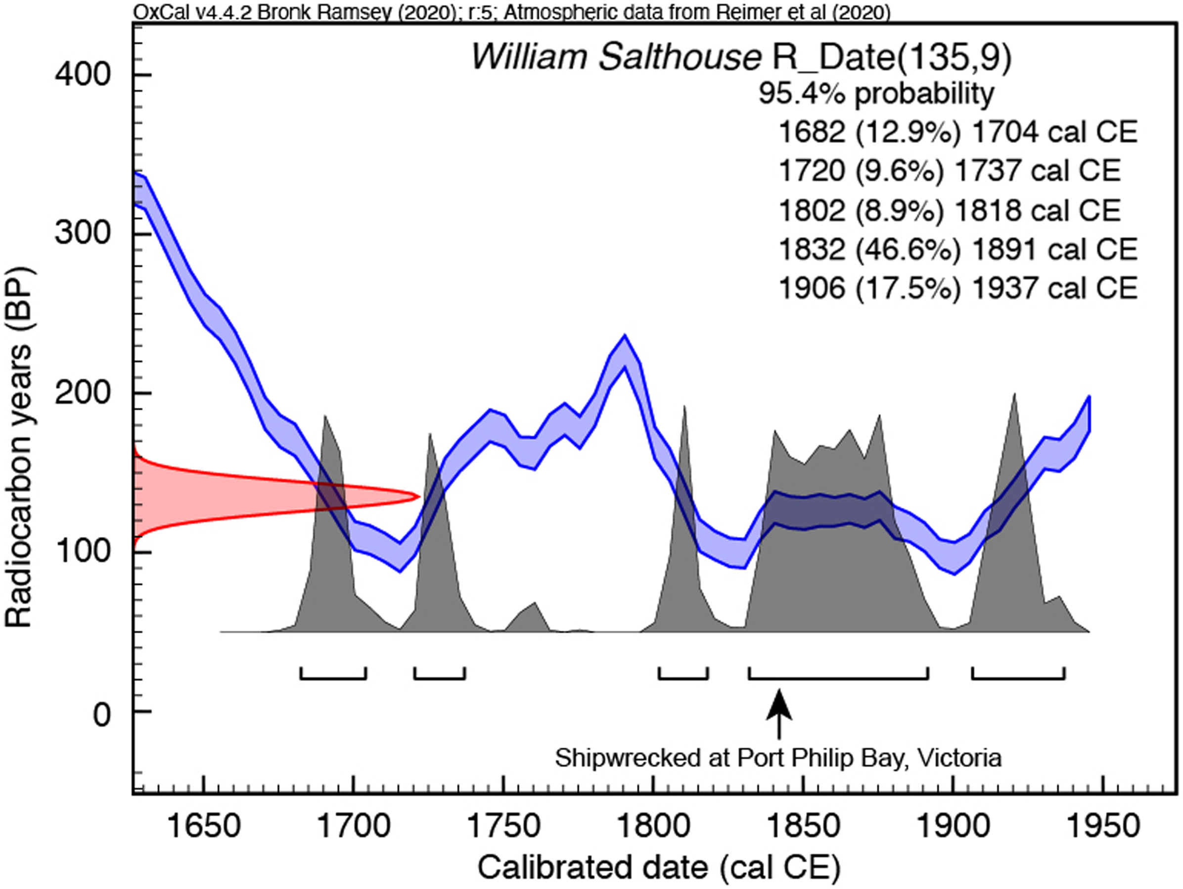
Figure 5 Calibration of Canadian cow bone from the 1841 William Salthouse shipwreck (Port Philip Bay, Victoria, Australia), an internal standard. Radiocarbon age calibration using IntCal20 (Reimer et al. Reference Reimer, Austin, Bard, Bayliss, Blackwell, Bronk Ramsey, Butzin, Cheng, Edwards and Friedrich2020) and OxCal version 4.4 (Bronk Ramsey and Lee Reference Bronk Ramsey and Lee2013).
Table 4 Mean and standard deviation (1 σ) stable isotope and elemental values for Hollis Mammoth and the William Salthouse Shipwreck cow. %C and %N are the percentages of carbon and nitrogen in the combusted sample. C:N, atomic weight ratio of carbon to nitrogen. Stable isotope ratios are expressed in per mil (‰), relative to VPDB and atmospheric N2 (AIR). The number in parentheses denotes the number of measurements used to generate weighted-average values.

Intercomparison
Accuracy at Chronos was investigated by measuring a suite of contiguous tree-ring cellulose samples across selected time periods. Intercomparisons were carried out between the Chronos facility and three other institutes: the Swiss Federal Institute of Technology (ETH), University of California, Irvine (UCI), and the University of Waikato (Waikato) (Figure 6). Measurements and sample processing methods from UCI and Waikato are published by (Hogg et al. Reference Hogg, Southon, Turney, Palmer, Bronk Ramsey, Fenwick, Boswijk, Friedrich, Helle and Hughen2016a, Reference Hogg, Southon, Turney, Palmer, Ramsey, Fenwick, Boswijk, Büntgen, Friedrich and Helle2016b) and (Turney et al. Reference Turney, Palmer, Maslin, Hogg, Fogwill, Southon, Fenwick, Helle, Wilmshurst and McGlone2018), respectively. Chronos and ETH results are presented in this study. The ETH protocol for wood is similar to that described above and published previously (Sookdeo et al. Reference Sookdeo, Kromer, Büntgen, Friedrich, Friedrich, Helle, Pauly, Nievergelt, Reinig and Treydte2020).

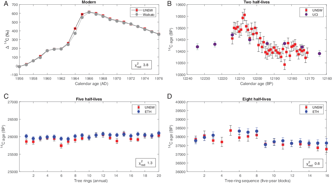
Figure 6 Intercomparison of tree ring 14C measurements from selected time periods: (A) UNSW Δ14C values (red) determined for the Bomb Peak (“Modern”) samples of subantarctic Dracophyllum scoparium that were previously measured by the University of Waikato/UCI (gray) (Turney et al. Reference Turney, Fogwill, Palmer, van Sebille, Thomas, McGlone, Richardson, Wilmshurst, Fenwick and Zunz2017, Reference Turney, Palmer, Maslin, Hogg, Fogwill, Southon, Fenwick, Helle, Wilmshurst and McGlone2018). (B) Annual 14C ages obtained from New Zealand kauri (Towai) determined by UNSW (red) for a selected period within the Younger Dryas chronozone (approximately two half-lives), previously measured decadally by UCI (black) (Hogg et al. Reference Hogg, Southon, Turney, Palmer, Bronk Ramsey, Fenwick, Boswijk, Friedrich, Helle and Hughen2016a, Reference Hogg, Southon, Turney, Palmer, Ramsey, Fenwick, Boswijk, Büntgen, Friedrich and Helle2016b; Palmer et al. Reference Palmer, Turney, Cook, Fenwick, Thomas, Helle, Jones, Clement, Hogg and Southon2016). (C) 14C ages from Waipu kauri determined to be approximately 25,000 years old (approximately five half-lives) at UNSW (red) and ETH (blue). (D) 14C ages determined for the Ngāwhā Springs approximately 40,000 years old (approximately eight half-lives) kauri samples at UNSW (red) and ETH (blue). Uncertainties are given as 1 σ.
University of Waikato
Samples measured by Waikato covered the thermonuclear weapons testing period between CE 1956 to 1976 that created a peak in atmospheric 14C. The so-called Bomb Peak resulted from anthropogenic stratosphere 14CO2, that transferred down into the troposphere. Through the late Northern Hemisphere spring exchange of air masses, zonal mixing and meridional atmospheric circulation, bomb related-14C was globally distributed (Dutta Reference Dutta2016). The resulting peak in atmospheric 14C has been detected in tree-rings that grow on the remote subantarctic Campbell Island in the southwest Pacific (Turney et al. Reference Turney, Palmer, Maslin, Hogg, Fogwill, Southon, Fenwick, Helle, Wilmshurst and McGlone2018). Here we focussed on an individual of Dracophyllum scoparium, one of a pair of related native tree species that are the most poleward growing in the southwest Pacific Ocean (Southern Ocean) and have been investigated as part of a previous study (Turney et al. Reference Turney, Fogwill, Palmer, van Sebille, Thomas, McGlone, Richardson, Wilmshurst, Fenwick and Zunz2017).
Our intercomparison results show an initial reduced χ2 of 29 (n-1 = 20). Removing the largest laboratory offsets, which occurred between CE 1964–1965, the reduced χ2 improves to 3.8 (n-1 = 18). It is likely that the offset across these two years of growth may be due to inconsistent tree-ring sampling in either this study or the previously published work (Turney et al. Reference Turney, Palmer, Maslin, Hogg, Fogwill, Southon, Fenwick, Helle, Wilmshurst and McGlone2018). Around the time of the Bomb Peak, ring boundaries that may have been inadvertently incorporated into an adjoining growing season have the potential to skew the radiocarbon measurement (Turney et al. Reference Turney, Palmer, Maslin, Hogg, Fogwill, Southon, Fenwick, Helle, Wilmshurst and McGlone2018); alternatively, given the rapid large changes in atmospheric 14C, part of the growing season may have been missed. This is particularly true for the period 1964–1965, which experienced the steepest rise in atmospheric 14C across the Bomb Peak and showed the largest laboratory offset (Figure 5a). Overall, however, the consistent values obtained from the two sets of analyses provides confidence that Chronos is capable of measuring twentieth century changes in atmospheric radiocarbon.
University of California, Irvine
We also undertook analyses on ancient kauri samples from Towai in Northland, New Zealand (35.5066˚S, 174.1729˚E), that span the Younger Dryas chronozone (Hogg et al. Reference Hogg, Southon, Turney, Palmer, Bronk Ramsey, Fenwick, Boswijk, Friedrich, Helle and Hughen2016a; Hogg et al. Reference Hogg, Southon, Turney, Palmer, Ramsey, Fenwick, Boswijk, Büntgen, Friedrich and Helle2016b; Palmer et al. Reference Palmer, Turney, Cook, Fenwick, Thomas, Helle, Jones, Clement, Hogg and Southon2016). In the North Atlantic region, the Younger Dryas was characterized by a millennial-long cold period that started approximately 12,900 calendar years ago, accompanied by globally rising atmospheric CO2 concentrations and warming across the mid- to high latitudes of the Southern Hemisphere (WAIS Divide Project Members 2015; Fogwill et al. Reference Fogwill, Turney, Menviel, Baker, Weber, Ellis, Thomas, Golledge, Etheridge and Rubino2020). The14C data measured at Chronos is sourced from the same tree as previously measured at UCI but subsampled at annual rather than decadal resolution. A χ2 test was not conducted on these samples as the number of data points is insufficient (n-1=3). Annual 14C data followed trends of the decadal measurements from UCI, particularly across the radiocarbon plateau, spanning 12,200–12,170 cal BP (Figure 5b). A depletion in atmospheric 14C is evident in the annual 14C data, which is not seen in the decadal 14C measurements from UCI. This is interpreted as interannual variations captured in our record but averaged out in the decadal data from UCI.
Swiss Federal Institute of Technology (ETH)
As part of our intercomparison, two sets of kauri samples—the first set from five half-lives and the other from approximately eight half-lives ago—were analyzed at Chronos and ETH (Figure 5C and D, respectively). The first set was obtained from a tree excavated at Waipu, a site on the east coast in Northland (35.9517ºS, 174.4497ºE), and the second from Ngāwhā Springs, also in Northland (35.4027ºS, 173.8586ºE). As these samples did not have an absolute calendar age, 14C ages were plotted against consecutive sample numbers. The Chronos results show excellent agreement with ETH’s results for both time periods.
The first set of intercomparison results from Waipu produced a reduced χ2 of 1.3 (n = 20). The uncertainties are improved further when sample 1184, which had the largest laboratory offset, is removed. The second set of intercomparison results from Ngāwhā Springs produced a reduced χ2 of 0.6 (n = 14), demonstrating a very good agreement of the datasets. The measured uncertainties may be considered relatively large not only because of the contribution of counting statistics (13–15‰) but also of the contribution of the estimated population uncertainty of cellulose blanks (±0.0004 in F14C) (Sookdeo et al. Reference Sookdeo, Kromer, Büntgen, Friedrich, Friedrich, Helle, Pauly, Nievergelt, Reinig and Treydte2020). Importantly, this reveals that samples such as these should be run in duplicate to better constrain 14C uncertainties.
CONCLUSIONS
This paper reports the pretreatment methods, preliminary results, and reporting protocols for the new Chronos 14Carbon-Cycle Facility, at the University of New South Wales. Built around an Ionplus 200 kV MIni-CArbon DAting System (MICADAS) AMS, the facility has now been operating since late 2019. In this time, we have been able to demonstrate radiocarbon and stable isotope measurements for a range of material types: bones, carbonates, peat, pollen, charcoal, and wood. A combination of international standards, samples of known-age, and blanks provides confidence in the Chronos Facility being capable of measuring 14C samples from the Anthropocene to nearly 50,000 years ago. Future work will focus on refining these methods and exploring other sample types (e.g., dissolved inorganic and organic carbon in water) that are critical for improving our understanding of the Earth system and managing resources in a future warmer world.
ACKNOWLEDGMENTS
We would like to acknowledge the support of the University of New South Wales through the 2025 Strategic Plan, in particular Professor Nick Fisk and Professor Grainne Moran. We would also like to thank our many friends and colleagues who have supported the development of the Chronos 14Carbon-Cycle Facility at UNSW, including those who kindly provided samples and/or expert advice: Anne-Louise Muir and Steven Avery (Heritage Victoria); John Southon and Hector Martinez de la Torre (University of California, Irvine); Tim Cohen and Matt Forbes (University of Wollongong); Peter Ditchfield and Tom Higham (University of Oxford); Francisca Santana Sagredo (Pontifical Catholic University of Chile); Petra Vaiglova (Washington University in St. Louis); Gerde Helle (GFZ German Research Centre for Geosciences, Potsdam); Quan Hua (ANSTO), and, Joël Bourquin, Simon Fahrni and the team at Ionplus (Zurich, Switzerland). ZT is supported by the Australian Research Council (DE200100907). We thank two anonymous reviewers who provided constructive comments that helped improve this manuscript