


Introduction
The evolution of the Polar Regions is an important scientific and societal issue in the context of global climate change. Turner et al. (Reference Turner, Lachlan-Cope, Colwell, Marshall and Connolley2006) have shown that the extreme conditions encountered in high latitudes make these places more sensitive to global warming, and the responses of the temperature variations are faster than at the mid-latitudes. They reported that the warming of the Antarctic winter troposphere is larger than anywhere else on Earth with a rate of 0.5–0.7 K per decade. However, the physical processes that rule the polar climate are still misunderstood and poorly represented in models (Hines et al. Reference Hines, Bromwich, Rasch and Iacono2004).
Several studies have already shown the extreme difficulty of models and analyses (assimilation of measurements into models) to represent the time evolution of the Antarctic atmosphere as measured by different sensors at different time scales, regarding the diurnal cycle (e.g. Genthon et al. Reference Genthon, Town, Six, Favier, Argentini and Pellegrini2010), the seasonal evolution (e.g. Tomasi et al. Reference Tomasi, Petkov and Benedetti2012), and the intra-seasonal variability (e.g. Argentini et al. Reference Argentini, Pietroni, Mastrantonio, Viola and Zilitinchevich2007), considering both the planetary boundary layer, the free troposphere or the upper troposphere-lower stratosphere. One of the caveats of the models is that they need to be constrained by measurements that are not well distributed at the surface of the Antarctic continent, mainly localized at coastal regions. Space-borne sensors can indeed fill this gap. One of the caveats of the space-borne sensors, particularly in the infrared (IR) domain, is that they are highly affected by the actual surface emissivity and albedo values of the Antarctic Plateau that strongly impact the retrievals of temperature and water vapour (H2O). They are also affected by chemical constituents (e.g. ozone and carbon monoxide) and clouds.
Water vapour is the main greenhouse gas emitting and absorbing IR radiation. Change of its abundance directly impacts the radiative balance of the Earth system, thus affecting the climate evolution (see e.g. Brasseur et al. Reference Brasseur, Orlando and Tyndall1999). Conversely, climate change will also impact the water budget of the Earth system. It is thus an important issue to study both H2O and temperature in such remote and climatically-sensitive regions.
The Dome C station (Concordia Station) in Antarctica (75°06′S, 123°21′E, 3233 m above mean sea level (a.m.s.l.)) has a unique opportunity to actually test the quality of the measurements and meteorological analyses because of its location well inside the East Antarctic Plateau (average altitude 2500 a.m.s.l.), and consequently can be considered as less affected by local phenomena such as e.g. orographic waves, katabatic winds, oceanic breeze, etc. that are far more prominent at coastal stations. The Antarctic Plateau is one of the coldest and driest places around the world. For these reasons, numerous atmospheric studies took place and are nowadays taking place, focused on e.g. reactive species interacting with snowpack (e.g. Davis et al. Reference Davis, Nowak, Chen, Buhr, Arimoto, Hogan, Eisele, Mauldin, Tanner, Shetter, Lefer and McMurry2001, Jones et al. Reference Jones, Weller, Anderson, Jacobi, Wolff, Schrems and Miller2001) and site seeing investigations for astronomical purposes (e.g. Aristidi et al. Reference Aristidi, Agabi, Vernin, Azouit, Martin, Ziad and Fossat2003, Tremblin et al. Reference Tremblin, Minier, Schneider, Durand, Ashley, Lawrence, Luong-van, Storey, Durand, Reinert, Veyssiere, Walter, Ade, Calisse, Challita, Fossat, Sabbatini, Pellegrini, Ricaud and Urban2011, De Gregori et al. Reference De Gregori, De Petris, Decina, Lamagna, Pardo, Petkov, Tomasi and Valenzano2012).
Furthermore, space-borne measurements, particularly in the ultraviolet-visible and IR domains and in the nadir-viewing direction, are very sensitive to surface emission and albedo that directly impact the retrievals. The Dome C station is located on a wide and rather homogeneous (in terms of surface emissivity and albedo) plateau. Thus, when comparing with space-borne measurements (by considering measurements within a circle of about 100 km or a box 2° x 2° centred at the Dome C station), retrievals are less affected by these surface inhomogeneities, and the associated statistics (mean, standard deviation, etc.) are meaningful. Finally, any instrument has its own strengths and weaknesses, and it is also a key issue of this manuscript to identify these terms when performing comparisons.
The aim of the present paper is twofold: 1) to assess the quality of the different H2O and temperature datasets available over one year, namely 2010, above the station of Dome C by performing a rigorous statistical analysis, and 2) to study the temperature vs H2O correlation over the entire troposphere and discuss the processes that produce the observed variability and correlations. To achieve this goal, we use standard statistical tools, such as mean, bias, standard deviation and linear Pearson correlation coefficient, calculated over three different seasons: summer, autumn/spring and winter; although we separated autumn and spring when considering temperature fields in the upper troposphere-lower stratosphere. Unfortunately, all the datasets are not available at the same local time, that is particularly important in the planetary boundary layer in summer due to the strong diurnal cycle in temperature and H2O (Ricaud et al. Reference Ricaud, Genthon, Durand, Attié, Carminati, Canut, Vanacker, Moggio, Courcoux, Pellegrini and Rose2012). Consequently, we have decided to consider, as a reference, the measurements from one specific instrument, namely the ground-based microwave radiometer H2O Antarctica Microwave Stratospheric and Tropospheric Radiometer (HAMSTRAD). This radiometer is able to sample the whole 24-hour diurnal cycle with a seven minute integration time from mid-January 2010 to end of December 2010, and from 0 m to 10 km above surface, with a vertical resolution from ∼30 m in the planetary boundary layer to ∼500 m in the upper troposphere-lower stratosphere (Ricaud et al. Reference Ricaud, Gabard, Derrien, Chaboureau, Rose, Mombauer and Czekala2010a, Reference Ricaud, Carminati, Attié, Courcoux, Rose, Genthon, Pellegrini, Tremblin and August2013). From previous studies (Ricaud et al. Reference Ricaud, Gabard, Derrien, Attié, Rose and Czekala2010b, 2012, 2013), we already know the strengths and weaknesses of this instrument that will be discussed later. The other datasets used in our study are: radiosondes, in situ sensors, the two IR space-borne sensors: Infrared Atmospheric Sounding Interferometer (IASI) on the MetOp-A platform and Atmospheric InfraRed Sounder (AIRS) on the Aqua platform, and, finally, the analyses from the European Centre for Medium-Range Weather Forecast (ECMWF).
The article is structured as follow. We present the different instruments involved in this study, namely HAMSTRAD, radiosondes, in situ sensors, space-borne sensors (IASI and AIRS) and ECMWF analyses. The statistical analyses in terms of yearly evolution, mean and bias, standard deviation and correlation are shown and discussed for tropospheric temperature, integrated water vapour (IWV) and tropospheric H2O. This is followed by discussion and conclusions.
Datasets
HAMSTRAD
The HAMSTRAD instrument is a radiometer developed by the Radiometer Physics GmbH German Company (Ricaud et al. Reference Ricaud, Gabard, Derrien, Chaboureau, Rose, Mombauer and Czekala2010a). Its goal is to sound the troposphere in very cold and dry environment to obtain temperature and absolute humidity profiles, together with IWV. The temperature profiles are derived using the 51–59 GHz spectral range, centred on the oxygen line. The absolute humidity profiles are retrieved using the 169–197 GHz spectral range, centred on the water vapour line. Integrated Water Vapour is calculated from the retrieved water vapour profile integrated along the vertical. Profiles can then be estimated from the surface to ten kilometres with a seven minute integration time. The instrument requires a liquid Nitrogen calibration one or two times per year. A comprehensive description of the instrument can be found in Ricaud et al. (Reference Ricaud, Gabard, Derrien, Chaboureau, Rose, Mombauer and Czekala2010a).
From February–June 2008, HAMSTRAD was firstly deployed at Pic du Midi station (42°56′N, 0°08′E, 2877 m a.m.s.l., France) for a first validation of water vapour measurements (Ricaud et al. Reference Ricaud, Gabard, Derrien, Attié, Rose and Czekala2010b). Then, the radiometer was sent to Dome C and installed outdoors in January 2009 for 12 days. Finally, after 16 January 2010, the instrument was deployed indoors inside a dedicated, equipped and heated container protected by a shield. It has been running automatically since then. The noise diode attached to the 183-GHz channels enabling automated calibration failed in June 2011, and was replaced in February 2012. Consequently, H2O measurements are not available over this period. This means the longest period available so far for a statistical comparison of H2O and temperature with other datasets covers the whole year of 2010.
Extensive validation and scientific studies have been performed in order to assess the quality of the measurements and to explain some physical processes from these measurements, mainly in the planetary boundary layer (Ricaud et al. Reference Ricaud, Genthon, Durand, Attié, Carminati, Canut, Vanacker, Moggio, Courcoux, Pellegrini and Rose2012). Regarding the quality of the measurements, Tables I & II show the 1-σ root mean square (RMS) random error, together with the vertical resolutions associated with the temperature and H2O profiles respectively, considering a seven minute integration time. Based on the statistical analyses performed in 2008 at the Pic du Midi station (Ricaud et al. Reference Ricaud, Gabard, Derrien, Attié, Rose and Czekala2010b), in January 2009 at Dome C (Ricaud et al. Reference Ricaud, Carminati, Attié, Courcoux, Rose, Genthon, Pellegrini, Tremblin and August2013) and considering the measurements performed in the planetary boundary layer in January–June 2010 (Ricaud et al. Reference Ricaud, Genthon, Durand, Attié, Carminati, Canut, Vanacker, Moggio, Courcoux, Pellegrini and Rose2012), some conclusions can be drawn regarding systematic biases of the HAMSTRAD measurements.
Table I Vertical resolutions and 1-σ root mean square (RMS) errors of temperature estimated for H2O Antarctica Microwave Stratospheric and Tropospheric Radiometer (HAMSTRAD), radiosonde, in situ sensor, Infrared Atmospheric Sounding Interferometer (IASI), Atmospheric InfraRed Sounder (AIRS) and European Centre for Medium-Range Weather Forecast (ECMWF) in the planetary boundary layer (PBL), in the free troposphere (FT) and in the upper troposphere-lower stratosphere (UTLS).

1Time and spatial resolutions are ∼7 min and ∼10 km eastward from the radiometer, respectively. Random errors are associated with a 7-min integration time.
2Vertical resolution estimated from yearly-averaged data representative of the year 2010 at Dome C.
3Note that the measurements from the nadir-viewing IR (infrared) sensors IASI and AIRS are usually insensitive to the PBL since its top height is less that 200–300 m except during the summer season when the PBL top height can be, on some occasions, higher (see e.g. Ricaud et al. Reference Ricaud, Genthon, Durand, Attié, Carminati, Canut, Vanacker, Moggio, Courcoux, Pellegrini and Rose2012).
Table II Vertical resolutions and 1-σ root mean square (RMS) errors of H2O estimated for H2O Antarctica Microwave Stratospheric and Tropospheric Radiometer (HAMSTRAD), radiosonde, in situ sensor, Infrared Atmospheric Sounding Interferometer (IASI) and Atmospheric InfraRed Sounder (AIRS), and European Centre for Medium-Range Weather Forecast (ECMWF) in the planetary boundary layer (PBL), in the free troposphere (FT) and in the upper troposphere-lower stratosphere (UTLS).

1Time and spatial resolutions are ∼7 min and ∼10 km eastward from the radiometer, respectively. Random errors are associated with a 7-min integration time.
2Vertical resolution estimated from yearly-averaged data representative of the year 2010 at Dome C.
3Note that the measurements from the nadir-viewing IR (infrared) sensors IASI and AIRS are usually insensitive to the PBL since its top height is less that 200–300 m except during the summer season when the PBL top height can be, on some occasions, higher (see e.g. Ricaud et al. Reference Ricaud, Genthon, Durand, Attié, Carminati, Canut, Vanacker, Moggio, Courcoux, Pellegrini and Rose2012).
To sum up, the instrument shows a very high sensitivity in the planetary boundary layer, a high sensitivity in the free troposphere and a very weak sensitivity in the upper troposphere-lower stratosphere. Below 4 km above surface, a 1–5 K cold bias is detected between HAMSTRAD and radiosonde measurements, and a warm bias above, of about 5–10 K. Integrated water vapour is of a high quality, namely about 1–2% wetter than radiosondes. Absolute humidity profiles are wetter by 0.1–0.3 g m-3 than radiosondes below about 2 km above surface and drier by ∼0.1 g m-3 above. Vertical resolution for both H2O and temperature measurements is ∼20–50 m in the planetary boundary layer, ∼100 m in the free troposphere and ∼500 m in the upper troposphere-lower stratosphere. Despite these known and well characterized biases, we have chosen to use HAMSTRAD measurements as reference since the instrument is the only device sampling the whole 24 hour diurnal cycle from the planetary boundary layer to the upper troposphere-lower stratosphere over the whole year 2010 with a high temporal sampling of approximately seven minutes. Consequently, HAMSTRAD measurements can be compared to the measurements of any other instrument in both time and space coincidences.
Radiosondes
Since spring 2005, a radiosonde is launched every day at 12h00 coordinated universal time (UTC) (20h00 Local Solar Time, LST) at Dome C. Measured profiles are integrated into the Global Telecommunication System of the World Meteorological Organization (WMO) and are validated before to be available on the Italian web site www.climantartide.it. Since 2009, the radiosonde type Vaisala RS-92SPGW is used and measures the temperature, pressure, relative humidity (with twin heated sensor) and wind thanks to an onboard GPS system. In our study, standard Vaisala evaluation routines are used to retrieve temperature and humidity profiles with no correction of time lag or sensor heating effect. Some corrections performed on the 2009 data according to Miloshevich et al. (Reference Miloshevich, Vömel, Whiteman, Lesht, Schmidlin and Russo2006) exhibited a weak impact (+4% maximum on IWV) on the vertical profiles in the troposphere (Ricaud et al. Reference Ricaud, Carminati, Attié, Courcoux, Rose, Genthon, Pellegrini, Tremblin and August2013). Using the procedure developed in Miloshevich et al. (Reference Miloshevich, Vömel, Whiteman and Leblanc2009), Tomasi et al. (Reference Tomasi, Petkov, Benedetti, Valenziano and Vitale2011, 2012) found that the corresponding correction factor for humidity provided by the RS92 at Dome C, for the 630–470 hPa layer and relative humidity level of 50–90%, varied between 1.10 and 1.15 for daytime and from 0.98–1.00 for night-time. The pressure range corresponds to a layer between the surface and about 2 km above the surface, which mainly contributes to the calculation of IWV. These values are consistent with the dry bias observed in the RS92 profiles from 5% at the surface to 40–50% in the upper troposphere-lower stratosphere (Miloshevich et al. Reference Miloshevich, Vömel, Whiteman, Lesht, Schmidlin and Russo2006, Rowe et al. Reference Rowe, Miloshevich, Turner and Walden2008). Regarding temperature, a cold bias is observed in the RS92 of 1.2 K up to 4 km above the surface (Tomasi et al. 2011, 2012). The 1-σ RMS errors (± 0.5 K) estimated by Vaisala on www.vaisala.com are reported in Table I. The 1-σ RMS errors for H2O are reported in Table II.
In situ sensors
In 2009, H2O and temperature in situ sensors were installed along a 45 m high tower. Ventilated PT100 and Humicap sensors were setup at 3.5, 10.6, 18.0, 25.3, 32.7 and 41.9 m along the tower (Genthon et al. Reference Genthon, Town, Six, Favier, Argentini and Pellegrini2010). Unlike Genthon et al. (Reference Genthon, Town, Six, Favier, Argentini and Pellegrini2010), the temperature sensors are PT100 DIN IEC 751 class 1/10 platinum thermistors with accuracy better than ±0.15°C at local temperatures. To prevent biases due to radiation contamination, sensors are shielded and force-ventilated using Young 43502 shields (Genthon et al. Reference Genthon, Six, Favier, Lazzara and Keller2011). The 1-σ RMS errors estimated by Genthon et al. (Reference Genthon, Town, Six, Favier, Argentini and Pellegrini2010) are reported in Table I. Vaisala HMP45ac and HMP155 thermo-hygrometers are deployed on the tower for the atmospheric moisture measure. Humicap capacitive hydro active sensors are also used which are a built-in part of the RS92 radiosondes produced by Vaisala and launched at Dome C (Genthon et al. Reference Genthon, Town, Six, Favier, Argentini and Pellegrini2010). The 1-σ RMS errors are reported in Table II. Note that data are not available in December 2010. The measurement frequency of the sensors is 0.1 Hz. Data are averaged within 30-min time bins and linearly interpolated and extrapolated at 10, 30 and 50 m above the surface.
IASI
IASI is an IR instrument onboard the space platform MetOp-A launched in 2006 (see e.g. http://smsc.cnes.fr/IASI;http://www.eumetsat.int/Home/Main/Satellites/Metop/Instruments/SP_2010053151047495). The platform has a sun-synchronous polar orbit inclined 98.7° to the Equator crossed (descending node) at 09h30 LST, at an altitude of about 815 km. The time for an orbit is 101 minutes with a repeat cycle of 29 days. Based on Michelson interferometer, IASI is an accurately calibrated Fourier Transform Spectrometer covering the 3.6–15.5 μm spectral range with 8400 spectral channels and a spectral resolution between 0.35 and 0.5 cm-1. IASI measures temperature and H2O with accuracies better than 1 K and 10%, respectively. The vertical resolutions and 1-σ RMS random errors estimated by Lerner et al. (Reference Lerner, Weisz and Kirchengast2002), Herbin et al. (Reference Herbin, Hurtmans, Clerbaux, Clarisse and Coheur2009) and Pougatchev et al. (Reference Pougatchev, August, Calbet, Hultberg, Oduleye, Schlussel, Stiller, St Germain and Bingham2009) are reported in Tables I & II for temperature and H2O, respectively.
Geophysical level 2 pre-operational data are provided by EUMETSAT (v4.3.2 from 21 January 2009, v4.3.3 from 29 March 2010 and v5.0.6 from 14 September 2010). They produce near-real time vertical profiles of temperature on a vertical pressure grid from 1000 to 0.1 hPa (Schlüssel et al. Reference Schlüssel, Hultberg, Phillips, August and Calbet2005, EUMETSAT 2012). The pressure grid is converted into an altitude grid by considering the hydrostatic equilibrium and the surface pressure and temperature. A 2° x 2° bin centred on the Dome C is considered for this study, where measurement times are in a range from 13h00–02h00 UTC (namely from 21h00–10h00 LST). The number of daily profiles averaged in a 2° x 2° bin is highly variable because only IASI data without cloud contamination in the line of sight are used along the large 2200 km swath of the scan.
AIRS
AIRS is an instrument onboard the space platform NASA EOS Aqua launched in 2002 (see http://airs.jpl.nasa.gov/). Together with the Advanced Microwave Sounding Unit and the Humidity Sounder for Brazil, they form an integrated cross-track scanning temperature and humidity sounding system. The platform has a sun-synchronous polar orbit with 14 orbits per day and equatorial crossing at 13h30 LST ascending node, at the altitude of about 705 km. A cross-track angle of sight of ±49° allows eight overpasses of Dome C each day around 07h00 and 19h00 UTC, with a resolution of 13.5 km at nadir and 41 x 21.4 km at the scan extremes (Aumann et al. Reference Aumann, Gregorich and Broberg2006).
AIRS is a high spectral resolution spectrometer working in the thermal IR which measures temperature with an accuracy of 1 K and H2O to better than 15% in layers 1 km thick in the free troposphere. The primary spectral calibration of the AIRS spectrometer, covering the 3.7–15.4 μm spectral range with 2378 spectral channels, is based on the cross-correlation between spectral features observed in the upwelling radiance spectrum with pre-calculated spectra (Aumann et al. Reference Aumann, Chahine, Gautier, Goldberg, Kalnay, McMillin, Revercomb, Rosenkranz, Smith, Staelin, Strow and Susskind2003, Divakarla et al. Reference Divakarla, Barnet, Goldberg, McMillin, Maddy, Wolf, Zhou and Liu2006). The vertical resolutions and 1-σ RMS errors estimated by Maddy & Barnet (Reference Maddy and Barnet2008), Tobin et al. (Reference Tobin, Revercomb, Knuteson, Lesht, Strow, Hannon, Feltz, Moy, Fetzer and Cress2006) and Arai & Liang (Reference Arai and Liang2009) are reported in Tables I & II for temperature and H2O, respectively.
The level 3 geophysical parameters (version 5) daily averaged and binned into 1° x 1° grid cells are provided by NASA on Giovanni, a web-based application developed by the GES DISC (Goddard Earth Sciences Data and Information Services Center; Susskind et al. Reference Susskind, Blaisdell and Iredel2010, NASA 2012). A 2° x 2° bin centred at the location of Dome C is considered for this study. Temperature profiles originally on a vertical pressure grid are converted into an altitude grid by considering the hydrostatic equilibrium and the surface pressure and temperature. We can separate AIRS data into ascending and descending nodes, corresponding to measurements performed in the vicinity of Dome C at 13h00 and 01h00 LST, respectively.
ECMWF
The ECMWF aims to develop numerical methods for meteorological forecast together with the collection and archive of meteorological data. The ECMWF analyses, hereafter called ECMWF, assimilate observations made worldwide into a meteorological model. The vertical resolution is distributed on 91 levels (from ∼8 m to ∼80 km), finest in the planetary boundary layer and coarsest in the stratosphere (see e.g. http://www.ecmwf.int/products/forecasts/guide/The_vertical_resolution.html). The horizontal resolution is approximately 50 km, but primitive equation variables are continuously defined through spherical harmonics. Tables I & II show the vertical resolutions together with the biases of the ECMWF analyses against radiosondes for temperature and H2O, respectively, at Dome C (Hagelin et al. Reference Hagelin, Masciadri, Lascaux and Stoesz2008). Four analyses are available per day at 00h00, 06h00, 12h00 and 18h00 UTC (namely, 08h00, 14h00, 20h00 and 02h00 LST).
Statistical analyses of tropospheric temperature
This section is dedicated to the statistical analysis of temperature. The different datasets used in our study have been seasonally averaged as follow: summer (January, February, November and December), autumn/spring (March, April, September and October) and winter (May, June, July and August). For one specific study (temperature evolution in the upper troposphere-lower stratosphere), we have separated the autumn (March and April) and the spring (September and October) seasons. We first present the yearly evolution of temperature as detected by the different sensors and analyses. Then, we show the mean seasonally-averaged profiles and biases, followed by the seasonally-averaged standard deviations and seasonally-averaged correlations. Note that height, within the entire manuscript, is defined as above the Dome C surface (unless specified).
Yearly evolution
Figure 1 shows the yearly evolution of the temperature as measured by the different instruments (HAMSTRAD, radiosondes, IASI and AIRS in ascending node) and analysed by ECMWF from January–December 2010. We can distinguish two main periods: 1) summertime (November, December, January and February) characterized by the highest temperatures, from ∼230–250 K in the planetary boundary layer and from ∼200–240 K in the upper troposphere-lower stratosphere, and 2) wintertime (May, June, July and August) characterized by the lowest temperatures, from ∼190–235 K in the planetary boundary layer and from ∼190–220 K in the upper troposphere-lower stratosphere. Autumn and spring (March–April and September–October, respectively) are short transition periods between high summer temperatures and low winter temperatures. This is indeed consistent with the analyses of radiosondes launched at Dome C from 2005–09 (Tomasi et al. Reference Tomasi, Petkov and Benedetti2012).
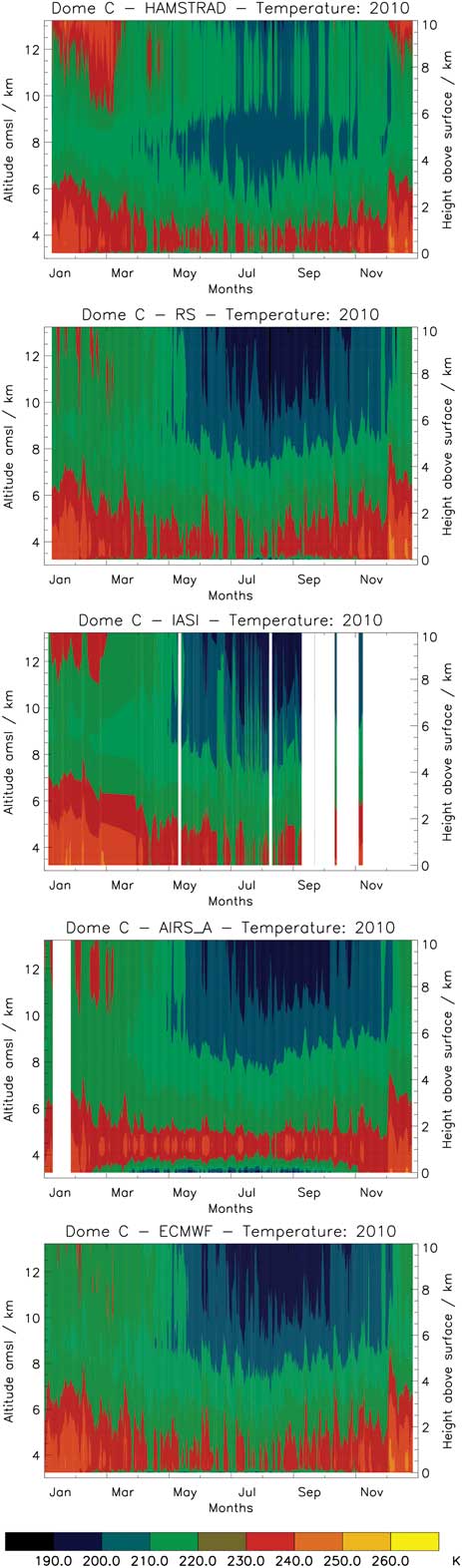
Fig. 1 From top to bottom: temporal evolution of temperature as measured by H2O Antarctica Microwave Stratospheric and Tropospheric Radiometer (HAMSTRAD), radiosonde (RS), Infrared Atmospheric Sounding Interferometer (IASI), Atmospheric InfraRed Sounder (AIRS) (ascending node) and the European Centre for Medium-Range Weather Forecast (ECMWF) analyses above Dome C from 1 January–31 December 2010. Note that, throughout the manuscript, when considering the vertical profiles, the figures display the altitude above mean sea level (km) on the left axis and the height above surface (km) on the right axis.
From the lowermost to middle troposphere, the temperature fields for all the datasets are symmetrical with respect to the winter period (July–August), whilst the fields are asymmetrical in the upper troposphere-lower stratosphere, with spring (< 210 K) much colder than autumn (> 210 K). This is related to the evolution of the polar vortex that builds up in the beginning of winter and collapses when air starts warming up in spring, see e.g. Ricaud et al. (Reference Ricaud, Lefevre and Berthet2005). In general, all the datasets behave consistently to each other, except for two main differences: 1) considering the HAMSTRAD dataset, the mid-to-upper troposphere is much warmer by about 10 K on average and the tropopause height is much lower by about 1–3 km than in all the other datasets, and 2) the lowermost troposphere as measured by AIRS in autumn/spring and winter is much colder by about 10–20 K than in all the other datasets. Another important point is the absence of IASI measurements above Dome C, mainly after 14 September 2010. On that particular date, the retrieval software developed at EUMETSAT was updated to v5.0.6 and pixels over icy surfaces were systematically but erroneously flagged as cloud-contaminated pixels, and consequently, not processed. Radiosonde and ECMWF temperature fields are very similar due to the assimilation of radiosondes launched at Dome C into the ECMWF analysis and forecast system.
Mean and bias
Figure 2 shows the seasonally-averaged temperature profiles as measured by the different instruments and analysed by ECMWF together with their absolute biases against the HAMSTRAD dataset. Biases against HAMSTRAD are calculated in temporal coincidence within a 60-min window, in summer, autumn/spring and winter. We have performed a sensitivity test considering a 30-min window instead of a 60-min window. The statistics remain unchanged with one major exception: the correlation between HAMSTRAD and in situ datasets in the planetary boundary layer in summer that is close to 1.0 in a 30-min window instead of 0.8–0.95 in a 60-min window. Indeed, the intense diurnal variation of temperature in the planetary boundary layer in summer (see Ricaud et al. Reference Ricaud, Genthon, Durand, Attié, Carminati, Canut, Vanacker, Moggio, Courcoux, Pellegrini and Rose2012), well depicted by the high temporal resolution of in situ and HAMSTRAD data, slightly affects the statistics in this case alone. From Fig. 1, we noticed that, in the upper troposphere-lower stratosphere, the temperature fields were not similar in autumn and in spring. Consequently, we have separated in Fig. 3 the seasonally-averaged temperature profiles from the different datasets in autumn and spring, together with the biases of all the datasets against the HAMSTRAD dataset.
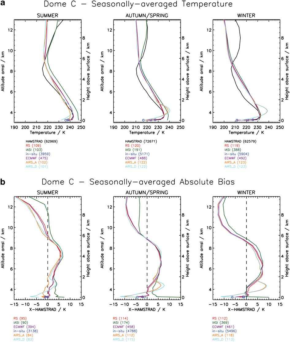
Fig. 2 a. From left to right: seasonally-averaged temperature profiles as measured by H2O Antarctica Microwave Stratospheric and Tropospheric Radiometer (HAMSTRAD) (black line), in situ (dark blue circles), radiosonde (RS) (red line), Infrared Atmospheric Sounding Interferometer (IASI) (green line), Atmospheric InfraRed Sounder (AIRS) in ascending node (orange line), AIRS in descending node (light blue line) and the European Centre for Medium-Range Weather Forecast (ECMWF) analyses (purple line) above Dome C in 2010 in summer, autumn/spring and winter. The number of profiles used in the seasonal average is indicated between brackets for each dataset. b. From left to right: same as in a. but for absolute biases of all the datasets vs HAMSTRAD dataset in temporal coincidence within a 60-min window.

Fig. 3 a. & b. As Fig. 2 but separating the autumn (left) and spring (right) seasons to highlight the different regimes in the upper troposphere-lower stratosphere.
In the lowermost troposphere, whatever the season considered, HAMSTRAD, in situ, radiosonde and ECMWF datasets are very consistent with each other showing a strong temperature gradient (from 235–243 K in summer and from 211–232 K in winter), from 10 to ∼900 m. Biases with respect to the HAMSTRAD dataset are from -1 to 1 K (± 0.5%) in summer and from -6 to 1 K (-2 to 0.5%) in winter. The temperature as measured by IASI is systematically high biased from 7–15 K (3–7%) with respect to HAMSTRAD measurements (∼247 K in the planetary boundary layer in summer) and IASI measurements do not show the strong temperature gradient previously highlighted from 10–900 m, particularly intense in winter due to the very cold surface temperature (see e.g. Genthon et al. Reference Genthon, Town, Six, Favier, Argentini and Pellegrini2010). The other space-borne IR instrument (AIRS), on the other hand, is able to catch such an intense temperature inversion in the planetary boundary layer, although the inversion zone in AIRS data is much higher (∼1 km) than in the other datasets (∼500 m) and much warmer by 1–7 K, depending on the season considered. Both AIRS and IASI measurements have very poor vertical resolutions (see Table I) of ∼1000 and ∼2500 m, respectively in the planetary boundary layer. In Ricaud et al. (Reference Ricaud, Carminati, Attié, Courcoux, Rose, Genthon, Pellegrini, Tremblin and August2013, appendix, part C), the impact of the vertical resolution on the vertical profiles has been investigated. A vertical resolution of 1000–2000 m can degrade the temperature in the planetary boundary layer and produces a positive bias of +6 to +7 K in summer, and up to +20 K (not shown) in winter, thus preventing the actual measurement of the temperature inversion. The AIRS results are thus consistent with our sensitivity study relative to the vertical resolution but not the IASI results. This probably means that IASI loses sensitivity in the planetary boundary layer above Dome C. On the other hand, in summer in the lowermost troposphere, the AIRS ascending temperature profiles are greater than the descending profiles by ∼5 K, with the ascending node measurements being closer to all the other datasets than the descending node measurements. Measurements of AIRS are performed at ∼13h00 LST in ascending node and ∼01h00 LST in descending node, thus the diurnal amplitude observed by AIRS is consistent with the ±5 K amplitude observed by ground-based instruments at Dome C in January (Ricaud et al. Reference Ricaud, Genthon, Durand, Attié, Carminati, Canut, Vanacker, Moggio, Courcoux, Pellegrini and Rose2012).
In the free troposphere (2–6 km above surface), all the datasets show a systematic 5–7 K (2.5–3%) positive bias with respect to the HAMSTRAD dataset, maximum between 4 and 4.5 km in summer, 3–3.5 km in autumn/spring and 2.5–3 km in winter. This means that the radiosonde, AIRS, IASI and ECMWF profiles are all consistent with each other to within ±1 K (1%).
In the upper troposphere-lower stratosphere (height > 6 km), the HAMSTRAD profile shows the minimum of temperature, characterizing the tropopause, at ∼5 km throughout the year, from 206 K (winter) to 215 K (summer), while the other instruments present a minimum at 5.5–6 km (217 K) in summer and above 10 km in winter. In autumn (Fig. 3), the minimum is at ∼5 km for all the datasets whilst, in spring, it is at ∼5 km in the HAMSTRAD dataset and above 10 km in all the other datasets. Above the tropopause, all the datasets (except IASI in summer and spring) present a systematic 9–14 K (3.5–6%) negative bias with respect to the HAMSTRAD measurements. When compared to all the other datasets except IASI, the shape of the HAMSTRAD profiles in summer, spring and winter seems unrealistic, with a strong gradient from the tropopause to the stratosphere whilst the HAMSTRAD profiles appear to be consistent with IASI in summer. This again confirms the previous studies stating that HAMSTRAD loses sensitivity in the upper troposphere-lower stratosphere. Above 6 km, radiosonde, AIRS and ECMWF agree to within 1–2 K.
Standard deviation
Figure 4 shows the seasonally-averaged absolute standard deviations as calculated for the different instruments and analysed by ECMWF in summer, autumn/spring and winter. In the lowermost troposphere, all the datasets (except IASI) show a strong gradient from the surface to 400 m, weak in summer from about 7.5 K at the surface to 5 K (3–2%) at 400 m and strong in winter from approximately 9.5 K at the surface to 4 K (3.8–1.6%) at 400 m. Note that, in conjunction with the maximum observed in the AIRS profile at ∼1 km and discussed in the previous section, a local minimum appears between 500 and 1000 m, ranging from 2.5 K (1%) in autumn/spring to 4 K (1.6%) in winter. Probably due to the IASI low sensitivity in the planetary boundary layer, the IASI standard deviation does not present any gradient in the lowermost troposphere but also within the whole troposphere in summer. This is unrealistic in summer (2.5 K instead of 4–6 K for all the other datasets) although in winter and, to a lesser extent, in autumn/spring, the IASI standard deviation is consistent with all the other datasets (4–6 K).

Fig. 4 As Fig. 2 but for absolute standard deviations of temperature.
In the free troposphere (1–5 km), all the datasets have a globally constant standard deviation, ranging from 4–5.5 K (1.6–2.2%) in summer and from 3–4 K (1.2–1.6%) in autumn/spring, except HAMSTRAD exhibiting an obvious maximum around 2–2.5 km approximately 0.5–1 K (0.2–0.4%) greater than all the other datasets. In the upper troposphere-lower stratosphere, the standard deviation of all the databases are all increasing with height, whatever the season considered, with values of 6–8 K around 8 km in summer and winter, up to 12 K in autumn/spring probably due to the breaking up of the vortex in spring.
The great variability observed in the planetary boundary layer cannot be entirely attributed to the diurnal variation of the solar radiation since it also persists in autumn/spring and winter. Preliminary studies presented in Ricaud et al. (Reference Ricaud, Carminati, Attié, Courcoux, Rose, Genthon, Pellegrini, Tremblin and August2013) attributed a great portion of the intra-seasonal variability to the origin of air masses coming from either the wet and warm oceanic areas or, dry and cold areas from the Antarctic plateau. Since the latitudinal gradient in temperature is more intense at the surface than in the middle troposphere, we can then expect to obtain greater standard deviations in the planetary boundary layer than in the free troposphere.
Correlation
Figure 5 shows the radiosonde, IASI, AIRS, in situ and ECMWF dataset correlation with respect to the HAMSTRAD dataset, calculated in temporal coincidence within a 60 min window. In the lowermost troposphere, whatever the season considered, the radiosonde, in situ, AIRS (in summer) and ECMWF datasets show a very high correlation > 0.8, greater than 0.9 in summer, with respect to the HAMSTRAD dataset. The correlation is very weak for IASI (0.2 in summer and 0.5 in winter and autumn/spring). From 0–2 km above surface, the IR space-borne instrument datasets (AIRS and IASI) give correlations systematically less than all the other datasets. This reinforces the point discussed in the previous section, namely that both the vertical resolution and the loss of sensitivity of IASI in the planetary boundary layer prevent the giving of meaningful information on temperature in the lowermost troposphere.
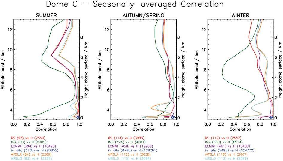
Fig. 5 As Fig. 2 but for correlation of H2O Antarctica Microwave Stratospheric and Tropospheric Radiometer (HAMSTRAD) temperatures vs all the other datasets in temporal coincidence within a 60-min window.
In the free troposphere, above 2 km, the correlation between the different datasets and the HAMSTRAD dataset is also high (> 0.8) except for IASI in winter (0.3–0.7). In summer, the IASI correlation is > 0.8 between 1.5 and 4 km, decreasing down to 0.4 at 5 km. The weak IASI correlation in winter (0.3) is rather intriguing and cannot be explained at the present time unless retrievals are greatly affected by an unsuitable surface emissivity used in the EUMETSAT retrieval software during this particular period when no solar radiation reaches the surface. A few months earlier, namely in autumn/spring and summer, the correlation coefficient is rather high (> 0.8) in the free troposphere, thus IASI gives meaningful information on mid-tropospheric temperature (see previous sections).
In the upper troposphere-lower stratosphere, correlations with HAMSTRAD are systematically lower than in the troposphere but nevertheless not negligible (0.6–0.8), with a local minimum around 6 km in summer (0.7 for the AIRS, 0.6 for the radiosonde and ECMWF datasets and 0.4 for IASI). Although HAMSTRAD loses sensitivity in this layer (Ricaud et al. Reference Ricaud, Carminati, Attié, Courcoux, Rose, Genthon, Pellegrini, Tremblin and August2013), it can nevertheless give meaningful information on temperature relative to, for example, time evolution and/or climatology. From surface to 10 km, ECMWF and radiosonde correlations are very similar in amplitude and shape, again underlining the fact that radiosondes launched at Dome C are used in the ECMWF analysis and forecast system. This underlines the great potential of HAMSTRAD measurements to validate both meteorological analyses and satellite measurements in such a remote place where very few independent data are available.
Statistical analyses of Integrated Water Vapour (IWV)
Yearly evolution
Figure 6 shows the temporal evolution of IWV above Dome C in 2010 as measured by HAMSTRAD, radiosonde, AIRS (ascending and descending nodes), IASI, and analysed by ECMWF. As expected from the time evolution of temperature (Fig. 1), a dry season is observed from May–August with values ranging from 0.05–0.6 kg m-2 and a wet (or less dry) season appears from November–February with values ranging between 0.4 and 1.5 kg m-2, showing some intense spikes in February and December with values > 2.1 kg m-2. We note the great consistency within all the datasets showing high (respectively weak) variabilities in summer (respectively winter) within a few days in agreement with Tomasi et al. (Reference Tomasi, Petkov and Benedetti2012).
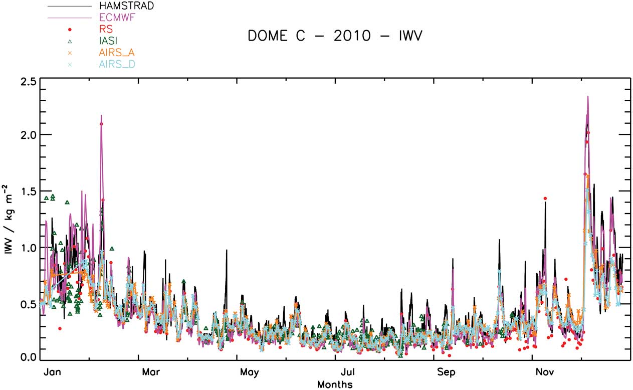
Fig. 6 Temporal evolution of the integrated water vapour (IWV) as measured by H2O Antarctica Microwave Stratospheric and Tropospheric Radiometer (HAMSTRAD) (black line), radiosonde (RS) (red dots), Infrared Atmospheric Sounding Interferometer (IASI) (green triangles), Atmospheric InfraRed Sounder (AIRS) ascending node (connected orange crosses), AIRS descending node (connected light blue crosses) and analysed by the European Centre for Medium-Range Weather Forecast (ECMWF) (purple line) above Dome C in 2010.
Bias
Figure 7 shows the IWV absolute biases of all the datasets with respect to the HAMSTRAD dataset selected within a 60-min time coincidence window. A systematic negative bias is observed in winter of about -0.03 ± 0.01 kg m-2 (-15 ± 5%) from May–August whilst, in summer, the negative bias reaches -0.1 ± 0.05 kg m-2 (-10 ± 5%). The 4–15% dry bias of the radiosondes during polar days is consistent with the 10–15% dry biases reported in Tomasi et al. (2011, 2012). We can note, in summer, the ECMWF bias is close to zero or slightly positive (0.06 kg m-2). The IASI strong negative biases (< -0.3 kg m-2) detected in October and November can certainly be attributed to the changes in the retrieval software at EUMETSAT that occurred on 14 September. The AIRS (ascending and descending nodes) biases in summer are systematically negative and much lower from -0.2 to -0.25 kg m-2 (approximately -20%) than the biases from all the other datasets, probably a signature of the impact of a misrepresentation of the surface emissivity and/or albedo in the retrieval software developed by NASA GES DISC.
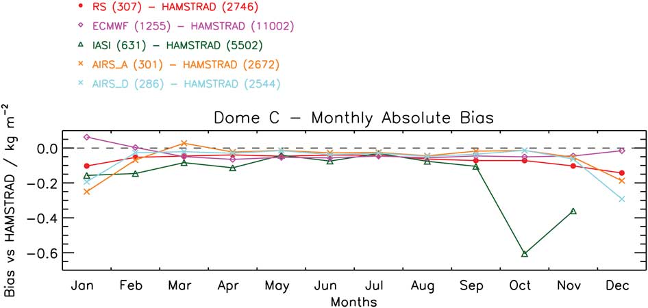
Fig. 7 Monthly-averaged integrated water vapour (IWV) absolute bias of H2O Antarctica Microwave Stratospheric and Tropospheric Radiometer (HAMSTRAD) against radiosonde (RS) (connected red circles), Infrared Atmospheric Sounding Interferometer (IASI) (connected green triangles), Atmospheric InfraRed Sounder (AIRS) ascending node (connected orange crosses), AIRS descending node (connected light blue crosses) and European Centre for Medium-Range Weather Forecast (ECMWF) (connected purple diamonds) above Dome C in 2010.
Standard deviation
The monthly-averaged absolute standard deviations of IWV from HAMSTRAD, radiosonde, AIRS (ascending and descending nodes), IASI and ECMWF datasets are presented in Fig. 8, showing a minimum in winter of ∼0.10 kg m-2 (35 ± 10%) and a maximum in summer of 0.15–0.55 kg m-2 (40 ± 10%). We can note a local maximum in February (0.4 kg m-2) as detected in the radiosonde and ECMWF datasets that is not present in all the other datasets.
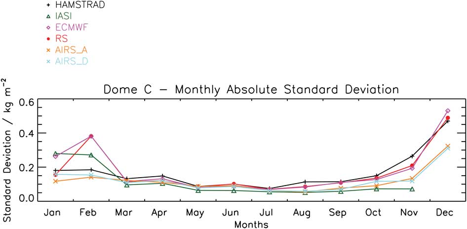
Fig. 8 As Fig. 7 but for integrated water vapour (IWV) absolute standard deviations.
Correlation
Figure 9 shows the IWV correlation of all the datasets calculated with respect to the HAMSTRAD dataset selected within a 60-min time coincidence window. On average, the correlation with HAMSTRAD is very high when considering the radiosondes (> 0.9) and the ECMWF (> 0.8) except in January (0.6), high when considering AIRS ascending and descending nodes (> 0.7) except in January (∼0.0 and -0.4, respectively), but lower when considering IASI in January, February, July, August and November (< 0.6), and slightly higher (∼0.7) in May, June, September and October.
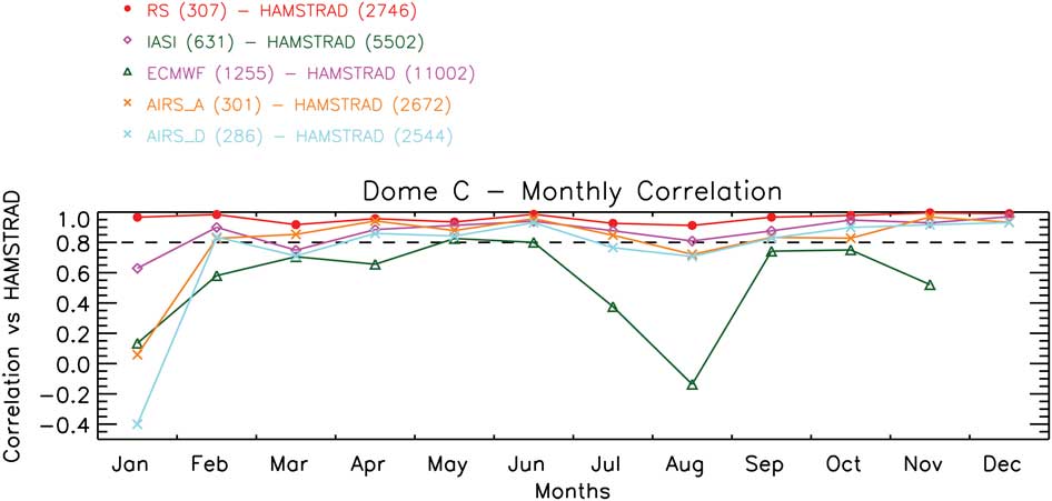
Fig. 9 As Fig. 7 but for integrated water vapour (IWV) correlation vs H2O Antarctica Microwave Stratospheric and Tropospheric Radiometer (HAMSTRAD).
Statistical analyses of tropospheric H2O
Yearly evolution
Figure 10 shows the temporal evolution of H2O above Dome C in 2010 as measured by HAMSTRAD, radiosonde, IASI, AIRS in ascending node and analysed by the ECMWF. As expected from the time evolution of IWV (Fig. 6), a wet season in summer followed by a dry season in winter is observed considering all the datasets with no obvious difference between autumn and spring patterns, consistent with Tomasi et al. (Reference Tomasi, Petkov and Benedetti2012). In summer, the amount of H2O is > 0.1 g m-3 from the surface to a height of about 2 km for HAMSTRAD and AIRS, reaching ∼3 km for radiosonde and ECMWF up to ∼4 km in the IASI dataset. In winter, HAMSTRAD and AIRS tend to measure H2O amounts (∼0.3 g m-3) much greater than all the H2O amounts from the other datasets (0.06 g m-3). As for temperature, IASI H2O measurements are missing after 14 September because of a change in the analysis software developed at EUMETSAT: icy pixels were usually considered as cloudy pixels and consequently not processed. Radiosondes and ECMWF H2O fields are indeed very similar, due to the assimilation of radiosondes launched at Dome C into the ECMWF analysis and forecast system.
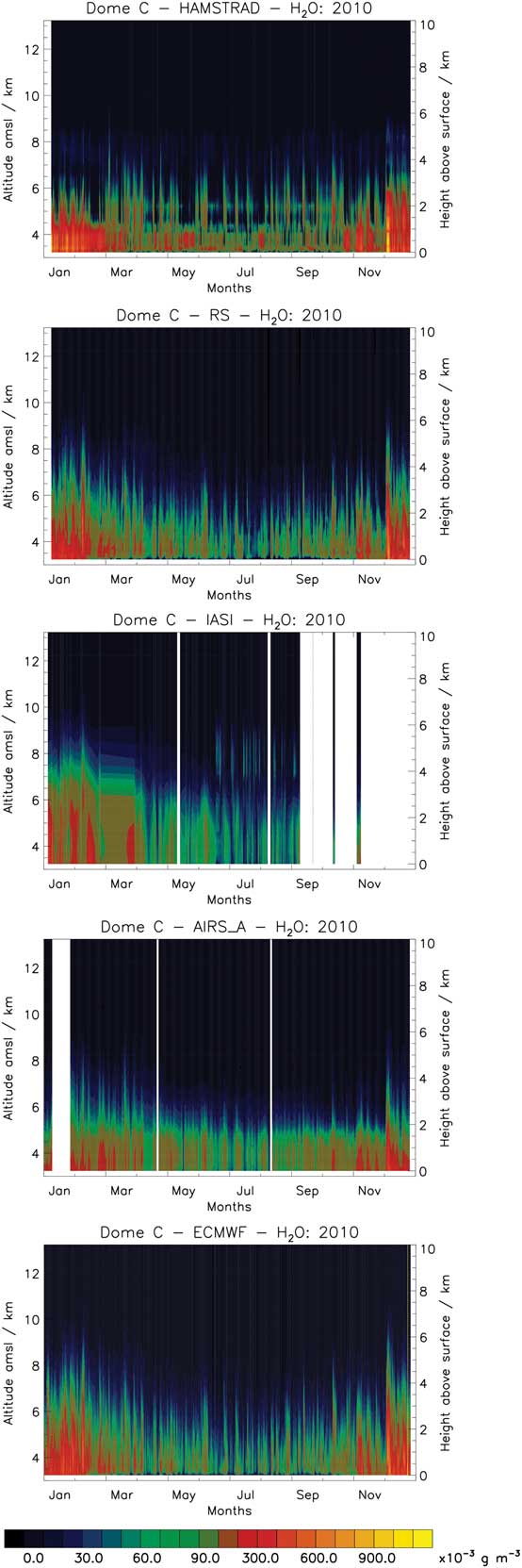
Fig. 10 From top to bottom: temporal evolution of the absolute humidity as measured by H2O Antarctica Microwave Stratospheric and Tropospheric Radiometer (HAMSTRAD), radiosonde (RS), Infrared Atmospheric Sounding Interferometer (IASI), Atmospheric InfraRed Sounder (AIRS) in ascending node and analysed by European Centre for Medium-Range Weather Forecast (ECMWF) above Dome C in 2010.
Mean and bias
Figure 11 shows the H2O seasonally-averaged profiles as measured by the different instruments and analysed by ECMWF, together with the biases against HAMSTRAD in temporal coincidence within a 60-min window. Below 500 m, we observe the wettest part of the atmosphere. Whatever the season considered, the H2O profiles from HAMSTRAD, radiosonde, in situ and ECMWF show a positive gradient from the surface to about 250 m, decreasing with altitude above 250 m. Profiles from the IR space-borne IR sensors IASI and AIRS do not exhibit such a sharp maximum but rather a wide and higher maximum as in winter and autumn/spring, or no maximum at all as in summer. The maximum amount of H2O is found in summer at ∼250 m from 0.2 g m-3 (IASI) to 0.5 g m-3 (HAMSTRAD), down to 0.06 g m-3 (IASI) to 0.16 g m-3 (HAMSTRAD) in winter. Note that in situ sensors always measure the driest atmosphere at 10 m (from 0.18 g m-3 in summer to 0.01 g m-3 in winter). In winter, the vertical profiles of all the datasets agree with each other to within 0.05 g m-3 whilst, in summer, the profiles agree to within 0.02 g m-3. As already shown in previous studies (Ricaud et al. Reference Ricaud, Carminati, Attié, Courcoux, Rose, Genthon, Pellegrini, Tremblin and August2013), compared to all the other datasets, HAMSTRAD tends to measure a wetter atmosphere below ∼2 km and drier above, whatever the season considered. Below 500 m, with the exception of HAMSTRAD (and IASI in summer), the absolute spread within all the datasets is very low in winter (0.02 g m-3) and higher in summer (0.05 g m-3), corresponding to a relative spread of ∼20% whatever the season considered.
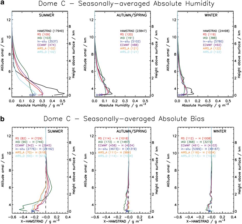
Fig. 11 a. From left to right: seasonally-averaged absolute humidity profiles as measured by H2O Antarctica Microwave Stratospheric and Tropospheric Radiometer (HAMSTRAD) (black line), in situ (blue circles), radiosonde (RS) (red line), Infrared Atmospheric Sounding Interferometer (IASI) (green line), Atmospheric InfraRed Sounder (AIRS) ascending node (orange line), AIRS descending node (light blue line) and analysed by European Centre for Medium-Range Weather Forecast (ECMWF) (purple line) above Dome C in 2010 in summer, autumn/spring and winter. The number of profiles used in the seasonal average is indicated between brackets for each dataset. Note that in a. the AIRS_D curve (orange line) is superimposed on the AIRS_A curve (light blue line). b. From left to right: same as in a. but for absolute biases of all the datasets against HAMSTRAD dataset in temporal coincidence within a 60-min window.
Above 500 m, all the datasets are consistent with each other and show a decrease of the H2O amount. The biases observed in summer are reduced, although IASI still measures the wettest atmosphere (up to 0.02 g m-3 wetter than HAMSTRAD measurements) from ∼2 km and AIRS the driest atmosphere (up to 0.04 g m-3 drier than HAMSTRAD measurements) from ∼1 km.
As for temperature (see Statistical analyses of tropospheric temperature, Mean and bias sub-section), both IASI and AIRS have very poor vertical resolution (see Table II) of ∼1000 m and ∼2700 m, respectively in the planetary boundary layer. Results presented in Ricaud et al. (Reference Ricaud, Carminati, Attié, Courcoux, Rose, Genthon, Pellegrini, Tremblin and August2013, appendix, part C) show that the impact of the vertical resolution of 1000–2000 m on the vertical profiles will degrade H2O amounts in the lowermost troposphere and will produce a positive bias of 20–30% in summer, and up to 100–120% in winter (not shown), thus preventing the actual measurement of the H2O gradient from the surface to ∼250 m. As for temperature, the AIRS H2O results are consistent with our sensitivity study relative to the vertical resolution but not the IASI results. This again shows that IASI loses sensitivity in the planetary boundary layer above Dome C.
Standard deviation
The absolute standard deviations of H2O as measured by HAMSTRAD, radiosonde, in situ, AIRS (ascending and descending nodes) and IASI, and analysed by ECMWF are presented in Fig. 12. The general shape is a vertical profile decreasing with height with an amplitude being much greater in summer (0.10–0.20 g m-3) than in winter (0.03–0.07 g m-3). Superimposed on that, some fine structures appear with local maxima at 200–500 m in HAMSTRAD, radiosonde, ECMWF and AIRS datasets in autumn/spring and winter, whilst in summer, the local maximum is close to the surface in radiosonde, AIRS and ECMWF datasets. The HAMSTRAD standard deviation is systematically much greater than all the other datasets, whatever the season considered, whilst. In summer AIRS standard deviation is systematically less than all the other datasets.
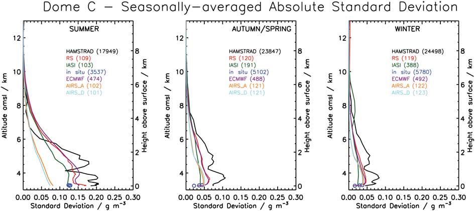
Fig. 12 As Fig. 11 but for absolute standard deviation of H2O.
Correlation
Figure 13 shows the H2O correlation with respect to height of the radiosonde, IASI, AIRS (ascending and descending nodes), in situ and ECMWF datasets against the HAMSTRAD dataset, calculated in temporal coincidence within a 60-min window. On average, the correlation ranges between -0.2 in the upper troposphere-lower stratosphere to +0.9 in the lower troposphere, that is to say the H2O datasets are less consistent than the temperature datasets. The highest correlation coefficients (0.7–0.9) are usually obtained close to the surface and at ∼1 km for radiosonde, ECMWF and AIRS, decreasing with height up to the upper troposphere-lower stratosphere where it can reach values close to zero or even negative (-0.2). We also can note a systematic minimum at 500 m whatever the season considered. The other datasets, namely AIRS, radiosondes, and ECMWF, are rather consistent with each other. This mainly confirms the fact that the HAMSTRAD H2O dataset is of a poorer quality compared to radiosonde, ECMWF and AIRS datasets. In summer, the IASI correlation departs considerably from all the other datasets but in winter IASI correlation below 1 km is consistent with AIRS, radiosondes, and ECMWF.
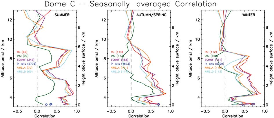
Fig. 13 As Fig. 11 but for H2O correlation of H2O Antarctica Microwave Stratospheric and Tropospheric Radiometer (HAMSTRAD) vs all the other datasets in temporal coincidence within a 60-min window.
Discussion: H2O vs temperature correlation
We have taken the opportunity of having access to a large dataset including both temperature and H2O measured and analysed simultaneously over one year and over a wide atmospheric layer (0–10 km) to check the correlation between these two parameters, and infer some conclusions about: 1) the quality of the datasets, and 2) the processes that could explain the correlation between temperature and H2O. Figure 14 shows the seasonally-averaged H2O vs temperature correlation calculated considering HAMSTRAD, radiosonde, in situ, AIRS (ascending and descending nodes), IASI and ECMWF databases.
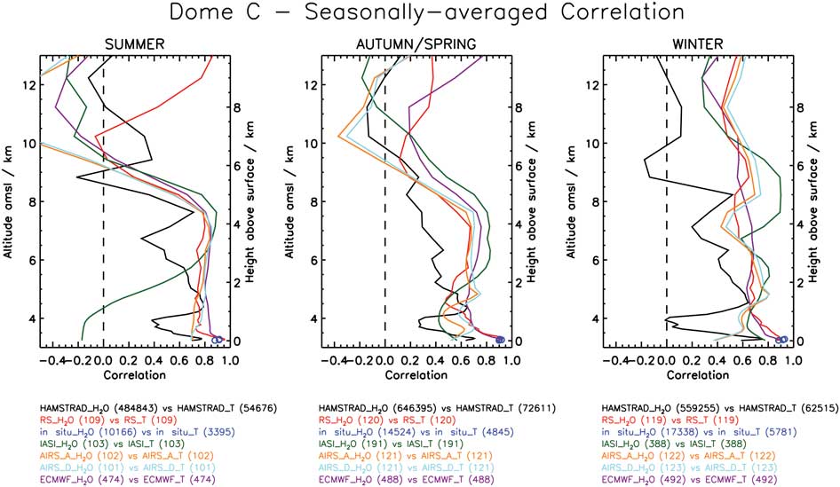
Figure 14 Seasonally-averaged correlation between temperature and absolute humidity as calculated for H2O Antarctica Microwave Stratospheric and Tropospheric Radiometer (HAMSTRAD) (black line), in situ (blue circles), radiosonde (RS) (red line), Infrared Atmospheric Sounding Interferometer (IASI) (green line), Atmospheric InfraRed Sounder (AIRS) ascending node (orange line), AIRS descending node (light blue line) and European Centre for Medium-Range Weather Forecast (ECMWF) (purple line) above Dome C in 2010.
Whatever the season considered, the correlation coefficient is generally > 0.7 from the surface to about 4–5 km for in situ, radiosonde and ECMWF datasets. It is much less for the HAMSTRAD dataset (0.4–0.8, even 0.0 at 500 m in winter), and IASI (0.4–0.8, even -0.2 below 1 km in summer). The best correlation coefficients are usually found close to the surface for in situ, radiosonde and ECMWF (0.9). We can observe an obvious transition in summer at 5 km with a correlation of almost null at 6 km, although in winter, the correlation is not negligible (∼0.5) in the upper troposphere-lower stratosphere (except for HAMSTRAD for which the correlation is almost null).
As discussed in the previous sections, the quality of the HAMSTRAD H2O measurements strongly impacts the weak values of the temperature vs H2O correlation whatever the altitude considered. In the lowermost troposphere, the space-borne IR sensors AIRS and IASI have little sensitivity due to their poor vertical resolution and this prevents high H2O vs temperature correlations. In the upper troposphere-lower stratosphere, HAMSTRAD measurements of H2O and temperature start losing sensitivity at ∼5 km above surface, consequently the H2O vs temperature correlation is rather low, oscillating around zero. Considering the other datasets in the upper troposphere-lower stratosphere, namely AIRS, IASI, radiosonde and ECMWF, we have checked (not shown) that, despite the fact that: 1) the amount of H2O is strongly decreasing, and 2) the vertical resolution of the space-borne sensors is rather poor, the time evolutions of H2O were consistent within all these datasets. This means that, on average, all these H2O measurements and analyses (except HAMSTRAD) are sensitive to the upper troposphere-lower stratosphere. Consequently, the H2O vs temperature correlation deduced from these datasets is meaningful in this altitude layer.
If we now concentrate on the datasets that give consistent results both in temperature and H2O, namely radiosonde, in situ, AIRS (excluding the lowermost troposphere) and ECMWF, the vertical distribution of H2O vs temperature can be represented in a schematic form (Fig. 15) by the season: summer, autumn/spring and winter. In general, we conclude that, in the troposphere, whatever the season considered, H2O and temperature are highly correlated (0.7–0.9), whilst, in the upper troposphere-lower stratosphere, the correlation is lost in summer (0.0–0.5) but still persists in winter (0.4–0.6) with a transition period in autumn/spring (0.2–0.6). Since the measurements of H2O and temperature can be considered as independent, we can investigate the processes that produce such a high correlation. In the planetary boundary layer, the H2O vs temperature correlation has been studied in detail by Ricaud et al. (Reference Ricaud, Genthon, Durand, Attié, Carminati, Canut, Vanacker, Moggio, Courcoux, Pellegrini and Rose2012) from summer to winter, namely from January–June 2010. Below 50 m, the high correlation (∼0.9) results partly from the fact that saturation vapour pressure increases with temperature. Thus the water-holding capacity of air correlates with temperature. Over one year in the entire troposphere, the seasonal cycle in temperature and H2O is induced by the seasonal cycle in solar radiation. Part of the variability in summer, and to a lesser extent in autumn/spring, is induced by the diurnal variability of the solar irradiance that produces an intense diurnal cycle in temperature and a weaker diurnal cycle in H2O, with a maximum lagged by 2–4 hours compared to local noon. In winter, such an explanation is irrelevant due to a lack of solar radiation. Nevertheless, the (intra-seasonal) variability is still strong as can be seen on Figs 4 & 12 for temperature and H2O respectively, with a temperature variability even greater in winter (8–10 K) than in summer (6–8 K). In Ricaud et al. (Reference Ricaud, Carminati, Attié, Courcoux, Rose, Genthon, Pellegrini, Tremblin and August2013), the variability of H2O and temperature over 12 days in January 2010 has been investigated by considering the origin of air masses. From the lowermost troposphere to the middle troposphere, using five-day back trajectories, it has been shown that wet and warm periods over Dome C were associated with air masses originating from oceanic wet and warm areas, and conversely, dry and cold periods over Dome C were obviously in phase with air masses originating from the cold and dry Antarctic plateau five days earlier. Furthermore, it also occurs that during cold and dry (warm and wet) periods, few warm and wet oceanic (cold and dry continental) air parcels interfere with the main stream, generating short events of one to ten-day duration characterized by simultaneous sharp increase (decrease) both in temperature and H2O with correlation > 0.8. Such a phenomenon has been studied in Ricaud et al. (Reference Ricaud, Carminati, Attié, Courcoux, Rose, Genthon, Pellegrini, Tremblin and August2013) and observed on 28 January 2009 when a cold and dry episode of two-day duration occurred during the summer warm and wet season.
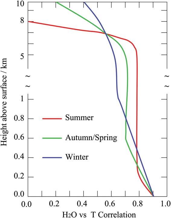
Figure 15 Schematic representation of the H2O vs temperature correlation along the vertical depending on the season: summer (red line), autumn/spring (green line) and winter (blue line).
In the upper troposphere-lower stratosphere, the H2O vs temperature correlation is definitely very low, essentially because processes occurring in this layer drastically differ from the tropospheric processes. Firstly, the stratosphere is strongly dehydrated by a factor of ∼10–100 less H2O in this layer than in the troposphere. Secondly, other processes occur depending on the season that strongly impact on the H2O budget. The vortex builds up in autumn and breaks down in spring. Subsidence induced by a very cold vortex appears in autumn and winter and produces a local rehydration. The presence of polar stratospheric clouds made of ice crystals in autumn/winter tends to dehydrate locally the lower stratosphere. Consequently, all these stratospheric processes tend to annihilate the high H2O vs temperature high correlation observed in the troposphere.
Conclusions
Measurements of tropospheric temperature and water vapour together with the IWV performed in 2010 at the Dome C station, Antarctica, are statistically analysed to assess their quality and to study the yearly correlation between temperature and H2O over the entire troposphere. The datasets are made of measurements from the ground-based microwave radiometer HAMSTRAD, radiosonde, in situ sensors, the space-borne IR sensors IASI on the MetOp-A platform and AIRS on the Aqua platform, and the analyses from the ECMWF.
First of all, two important points need to be stated for both temperature and H2O. The first point is the absence of IASI measurements above Dome C, mainly after 14 September 2010. On that particular date, the retrieval software developed at EUMETSAT has been updated to v5.0.6 and pixels over icy surfaces were systematically but erroneously flagged as cloud-contaminated pixels, and consequently, not processed. Secondly, radiosonde and ECMWF temperature fields are usually very similar due to the assimilation of radiosondes launched at Dome C into the ECMWF analysis and forecast system.
In general, all the temperature datasets behave consistently with each other, except for two main differences: 1) considering the HAMSTRAD dataset, the mid-to-upper troposphere is much warmer by about 10 K on average and the tropopause height is much lower by about 1–3 km than in all the other datasets, and 2) the lowermost troposphere as measured by AIRS in autumn/spring and winter is much colder by about 10–20 K than in all the other datasets. The strong temperature inversion observed in the lowermost troposphere by HAMSTRAD, radiosonde, in situ and ECMWF is also detected by AIRS (but higher and less intense) but not by IASI. Whilst the poor vertical resolution of the space-borne IR sensors (1000–2000 m) in the planetary boundary layer prevents the detection of such an intense gradient, IASI also seems to lack sensitivity within the surface layer.
In the lowermost and free troposphere, whatever the season considered, the radiosonde, in situ, AIRS (in summer) and ECMWF datasets show a very high correlation (> 0.8) with the HAMSTRAD dataset, except for IASI for which the correlation can be very low (0.2–0.7). In the upper troposphere-lower stratosphere, the correlation with HAMSTRAD is low (0.6–0.8). This reinforces the fact that the HAMSTRAD radiometer loses sensitivity in the upper troposphere-lower stratosphere.
All the IWV datasets are very consistent with each other showing a dry season from May–August with values ranging from 0.05–0.6 kg m-2 and a wet (or less dry) season from November–February with values ranging between 0.4 and 1.5 kg m-2, and some intense spikes in February and December with values > 2.1 kg m-2. A systematic negative bias of all the datasets against HAMSTRAD dataset is observed in winter of about -0.03 ± 0.01 kg m-2 (-15 ± 5%) whilst, in summer, the negative bias reaches -0.1 ± 0.05 kg m-2 (-10 ± 5%). The correlation with HAMSTRAD is very high when considering the radiosondes (> 0.9) and the ECMWF (> 0.8), high when considering AIRS ascending and descending nodes (> 0.7), but low when considering IASI (< 0.7).
A wet season in summer followed by a dry season in winter is observed considering all the datasets with no obvious difference between autumn and spring patterns. In summer, the amount of H2O is > 0.1 g m-3 from the surface to a height of about 2 km for HAMSTRAD and AIRS, reaching ∼3 km for radiosonde and ECMWF up to ∼4 km in the IASI dataset. In winter, HAMSTRAD and AIRS tend to measure H2O amounts (∼0.3 g m-3) much greater than all the H2O amounts from the other datasets (0.06 g m-3). Whatever the season considered, the H2O profiles from HAMSTRAD, radiosonde, in situ and ECMWF datasets show a positive gradient from the surface to about 250 m, decreasing with altitude above 250 m. This sharp surface gradient is missed by the two space-borne IR sensors IASI and AIRS due to the poor vertical resolution of 1000–2000 m.
The correlation between HAMSTRAD and all the other datasets ranged between -0.2 in the upper troposphere-lower stratosphere to +0.9 in the lower troposphere, which means that the H2O datasets are less consistent with each other than the temperature datasets. The highest correlation coefficients (0.7–0.9) are usually obtained close to the surface and at ∼1 km for radiosonde, ECMWF and AIRS, decreasing with height up to the upper troposphere-lower stratosphere where it can reach values close to zero or even negative (-0.2). Our study underlines the great potential of HAMSTRAD measurements to validate both meteorological analyses and satellite measurements in such a remote place where very few independent data are available.
Finally, we investigated the temperature vs H2O correlation within all the datasets. Whatever the season considered, the correlation coefficient is in general > 0.7 from the surface to c. 4–5 km for in situ, radiosonde and ECMWF datasets. It is much less for HAMSTRAD and IASI datasets (0.4–0.8). The highest correlation coefficients are usually found close to the surface for in situ, radiosonde and ECMWF (0.9). The quality of the HAMSTRAD H2O measurements strongly impacts the low values of the temperature vs H2O correlation. For the space-borne IR sensors AIRS and IASI, the poor vertical resolutions of their measurements prevents getting high temperature vs H2O correlations in the lowermost troposphere.
Over one year, the seasonal cycle in tropospheric temperature and H2O is induced by the seasonal cycle in solar radiation. Below 50 m, the high correlation (∼0.9) results partly from the fact that saturation vapour pressure increases with temperature. Thus, the water-holding capacity of air correlates with temperature. Part of the variability in summer is induced by the diurnal variability of the solar irradiance that produces an intense diurnal cycle in temperature and H2O (Ricaud et al. Reference Ricaud, Genthon, Durand, Attié, Carminati, Canut, Vanacker, Moggio, Courcoux, Pellegrini and Rose2012). But in winter, such an explanation is indeed irrelevant due to a lack of solar radiation. The intra-seasonal variability of H2O and temperature has already been investigated in Ricaud et al. (Reference Ricaud, Carminati, Attié, Courcoux, Rose, Genthon, Pellegrini, Tremblin and August2013) by considering the origin of air masses. From the lowermost troposphere to the middle troposphere, using five-day back trajectories, it has been shown that wet and warm periods over Dome C were associated with air masses originating from oceanic wet and warm areas, and conversely, dry and cold periods over Dome C were obviously in phase with air masses originating from the cold and dry Antarctic Plateau five days before. Such a preliminary study will need to be continued: i) to infer a climatological response to such a phenomenon based upon ECMWF analyses over a decade, and ii) to analyse case studies by using mesoscale models (e.g. AROME) in order to quantify the long-range transport of air masses upon the variabilities of temperature and H2O within the entire troposphere.
Acknowledgements
The HAMSTRAD programme (910) has been funded by the Institut National des Sciences de l'Univers (INSU)/Centre National de la Recherche Scientifique (CNRS), the Institut Polaire Français Paul-Emile Victor (IPEV) and the Centre National d'Etudes Spatiales (CNES). The permanently manned Concordia Station is jointly operated by IPEV and the Italian Programma Nazionale Ricerche in Antartide (PNRA). IASI has been developed and built under the responsibility of CNES. It is onboard the MetOp-A satellite as part of the EUMETSAT polar System. IASI vertical profiles of water vapour and temperature were extracted from the Ether French atmospheric database (http://ether.ipsl.jussieu.fr, accessed July 2013). AIRS has been developed and built under the responsibility of the National Aeronautics and Space Administration (NASA). It is onboard the NASA EOS Aqua satellite. AIRS data were extracted from Giovanni, a web-based application developed and maintained by the NASA GES DISC (http://gdata1.sci.gsfc.nasa.gov/daac-bin/G3/gui.cgi?instance_id=AIRS_Level3Daily, accessed July 2013). We finally would like to thank the three anonymous reviewers for their helpful comments.


