2. Comments on the database

The direct numerical simulation data are acquired from standard pseudo-spectral methods. The Taylor microscale Reynolds number ranges from ${R_\lambda }\sim 3$ to about $400$. The resolution is at least $k_{max}\eta \approx 3$ ($k_{max}=\sqrt {2}N/3$ is the highest wavenumber resolvable by the numerical scheme on a $N^3$ grid). This resolution is two to three times better than that commonly deemed as adequate for high-${R_\lambda }$ simulations; for the best resolved case, the resolution is as high as $k_{max}\eta \approx 35$. Time stepping is done via a second-order Runge–Kutta method with a constant step size chosen such that the Courant–Friedrichs–Lewy number for the database is kept near $0.3$ to accurately resolve extreme events (Yeung, Sreenivasan & Pope Reference Yeung, Sreenivasan and Pope2018). The flow is maintained stationary by forcing in the sphere $|{\boldsymbol k}|\leq 2$, where ${\boldsymbol k}$ is the wavenumber vector. The stochastic forcing (SF) scheme is based on Eswaran & Pope (Reference Eswaran and Pope1988) and has been used extensively in past studies. The deterministic forcing (DF) scheme, based on Donzis & Yeung (Reference Donzis and Yeung2010), maintains constant energy in the same low wavenumbers.

To remove dependencies on initial conditions, we have run the simulations for at least 8 eddy turnover times before statistics are collected. The duration of the simulations over which these statistics are computed is at least 15 eddy turnover times, which was found to be sufficient for statistical convergence. Simulation details are summarized in table 1.

Table 1. Direct numerical simulation database: the Taylor microscale Reynolds number is defined as ${R_\lambda }\equiv u_{rms}\lambda /\nu$, where $u_{rms}=(3/2)\overline {\langle u^2(\boldsymbol {x},t)\rangle }$ (brackets and an overline correspond to space and temporal averages, respectively), and the Taylor microscale $\lambda$ is defined using this velocity scale along with its time- and space-average gradient; $N^3$ is the grid resolution; $T_s$ is the duration of the stationary state normalized by the eddy turnover time $T_E\equiv L/u_{rms}$ ($L$ being the longitudinal integral length scale).

3. Single-time statistics

We recall that the three-dimensional energy spectrum $E(k,t)$ evolves according to

(3.1)\begin{equation} \frac{\partial E(k,t) }{\partial t}= T(k,t)-2 \nu k^2 E(k,t)+F(k,t), \end{equation}

where $T(k,t)$ is the inter-component and inter-scale energy transfer and $F(k,t)$ is the forcing applied at the low wavenumbers (§ 2). Our goal is to study the nature of $E(k,t)$ and $T(k,t)$ in different regions of the $k$-space, for the two forcing schemes of § 2. The fluctuations outside the forcing sphere $(k>k_f)$, in both $E$ and $T$, are comparable for the SF and DF cases at the same ${R_\lambda }$, even though the energy fluctuations within the forcing sphere $(k\leq k_f)$ are exactly zero for DF, suggesting that the fluctuations are the result of nonlinear dynamics of turbulence. Hence, for brevity, all the results presented here are for the SF forcing case.

We write the time average of $E(k,t)$ at a wavenumber $k$ as $E(k) \equiv \bar {E}(k,t) \equiv (1/T_s)\int _0^{T_s} E(k,t)\,\textrm {d} t$ and $T_s$ is the duration of averaging, as listed in table 1. Similar expressions hold for $T(k)$. Typical time series in energy $(E'(k,t)\equiv E(k,t)-E(k))$ and energy transfer $(T'(k,t)\equiv T(k,t)-T(k))$ are shown in figure 1, normalized by their respective averages. Energy transfer $T^\prime$ is an order of magnitude larger than the average, leading us to the first observation that the statistical mechanics of energy transfer is not unidirectional with minor fluctuations in time, but that of a system that fluctuates wildly around a much smaller time average. The energy itself varies considerably more mildly in the IR and the BR (an order of magnitude smaller than the average); we will attempt to explain this towards the end of § 4. As one approaches the NDR, fluctuations in energy transfer are highly correlated at all wavenumbers (figure 1c). Energy fluctuations in the NDR (figure 1d) are small and slow.

Figure 1. Time series of fluctuations in energy and energy transfer in the stationary state; (a–d) ${R_\lambda }\approx 390$. (a) Temporal change of the energy transfer at wavenumbers in the IR marked in the legend. The time average of the energy transfer has been subtracted, so the quantity presented is the deviation (or the fluctuation) from the average value, divided by the average. Note that the fluctuations are an order of magnitude larger than the average for the transfer. (b) Time series of energy at those same wavenumbers; the fluctuation is of the order of the average. The oscillatory blue line in (c) is the energy transfer in the BR, while the others approach the NDR; (d) time series for the energy. (e) Reynolds number ${R_\lambda }\approx 90$ and the data are in the FDR; (f) the behaviour close to the mean in (e). See text for more details.

Finally, in the FDR (figure 1e,f), we see highly intermittent variations in $T^\prime$, much stronger (relative to their averages) than those at lower wavenumbers, as also reported by Khurshid et al. (Reference Khurshid, Donzis and Sreenivasan2018). The variations are similar in $E^\prime$. Since the energy content in the dissipation range decays rapidly with increasing $k$, the energy and local transfer are very small and the signal is dominated by large intermittent fluctuations observed in figure 1(e,f). This behaviour was characterized in Khurshid et al. (Reference Khurshid, Donzis and Sreenivasan2018).

We now show in figure 2 the standard deviation ($\sigma (X) \equiv \sqrt {\overline {X'(k,t)^2}}$ with $X=E$ or $T$) in different wavenumber regions. In the IR, the fluctuations in $E$ (figure 2a) are substantially smaller than those in $T$ (figure 2b). All fluctuations become weaker as $k$ increases, reaching a minimum at ${k\eta }\sim 0.13$ for $E$, and, much more unambiguously, at ${k\eta }\sim 0.3$ for $T$, corresponding to the respective bottleneck peaks in their spectra (Falkovich Reference Falkovich1994; Verma & Donzis Reference Verma and Donzis2007; Donzis & Sreenivasan Reference Donzis and Sreenivasan2010; Ishihara et al. Reference Ishihara, Morishita, Yokokawa, Uno and Kaneda2016; Küchler et al. Reference Küchler, Bewley and Bodenschatz2019). Fluctuations in $T$ within the IR decay approximately as $k^{-5/3}$ for ${R_\lambda }\gtrsim 90$. The minimum in the variance of $E$ in the BR is consistent with Ishihara et al. (Reference Ishihara, Morishita, Yokokawa, Uno and Kaneda2016), who used a different forcing mechanism from those used here; this suggests that this minimum occurs independent of forcing. The fluctuations in $E$ were recently studied in the context of non-equilibrium corrections to the spectra by Bos & Rubinstein (Reference Bos and Rubinstein2017), who proposed that the ratio of non-equilibrium and equilibrium parts of the energy spectra scales as $k^{-2/3}$ in the IR. This scaling was also proposed by Yoshizawa (Reference Yoshizawa1994). Using slightly different arguments, Horiuti & Tamaki (Reference Horiuti and Tamaki2013) showed that this scaling is consistent with the transfer fluctuations decaying as $k^{-5/3}$ in the IR. This scaling of transfer fluctuations is consistent with the direct numerical simulation data in figure 2(b). Energy fluctuations, on the other hand, show a weaker decay (approximately $k^{-1/3}$) than predicted by the work cited above. This apparent discrepancy is discussed later in this section.

Figure 2. Normalized standard deviations $\sigma _{E}/E(k)$ (a) and $\sigma _{T}/T(k)$ (b). The vertical lines correspond to bottleneck peak in the energy spectrum (dotted, ${k\eta }=0.13$) and in the transfer spectrum (dashed-dotted, ${k\eta }=0.3$), and the boundary between the NDR and FDR (dashed, ${k\eta }=3$).

For wavenumbers beyond the BR, the relative fluctuations grow almost exponentially with the wavenumber in both the energy and transfer spectra. The presence of large and similar-level fluctuations in $T$ to either side of the BR is consistent with our understanding of the BR (Falkovich Reference Falkovich1994; Donzis & Sreenivasan Reference Donzis and Sreenivasan2010). It is also consistent with conclusions from Brasseur (Reference Brasseur1991) and Brasseur & Wei (Reference Brasseur and Wei1994) where the presence of significant non-local interactions between large and dissipative scales was observed; it is similarly consistent with Domaradzki (Reference Domaradzki1988), Domaradzki & Rogallo (Reference Domaradzki and Rogallo1990) and Domaradzki & Carati (Reference Domaradzki and Carati2007), where it was shown that non-local interactions in $T$ exhibited strong cancellations when averaged over all pertinent triads, weakening their overall effect in the IR.

We do not observe any statistically significant trends with respect to ${R_\lambda }$ for fluctuations in the dissipation range but a slight weakening occurs in the IR.

The main conclusion so far is that the fluctuations of energy transfer $T$ in the IR are large and fast, but those of the energy $E$ are moderate and slow. The fluctuations tend to be of the order of the average as one moves through the BR and then grow again in the NDR becoming large and fast in the FDR.

To pursue this point further, it is useful to separate the slow and fast frequencies demarcated by a frequency $\omega _c$ as

(3.2a,b)\begin{equation} \frac{E'(k,t)}{E(k)}=E'_{<}(k,t)+E'_{>}(k,t),\quad \frac{T'(k,t)}{T(k)}=T'_{<}(k,t)+T'_{>}(k,t), \end{equation}

where $E'_{<}(t)$ corresponds to the signal for $\omega <\omega _c$ and $E'_{>}(t)$ to that for $\omega >\omega _c$, and transfer signals follow the same convention. To be specific, we choose $\omega _c$ by decomposing the volume-averaged dissipation, $\langle \epsilon (t)\rangle$, into two parts such that the correlation between $\langle \epsilon (t)\rangle$ and its slow part is higher than $99\,\%$. This is readily done by Fourier-transforming the signals in time and adjusting the filter cutoff $\omega _c$. The decomposition into temporal frequencies is performed on variables ($E'(k,t)$, $T'(k,t)$ and $\langle \epsilon (t) \rangle$) computed from the full velocity field. A physical interpretation of slow and fast modes in terms of classical small and large scales is non-trivial and must invoke the concept of (random) sweeping (Kraichnan Reference Kraichnan1977).

In figure 3(a) we plot the slow part of fluctuations in energy transfer for ${R_\lambda }\sim 390$. A comparison with figure 1 shows that slow fluctuations are an order of magnitude smaller in the IR than the full signal, as emphasized by their standard deviations (solid line for the slow part and dashed line for the full signal in figure 3b). We reach the tentative conclusion here (and consolidate in the next section) that the notion of unidirectional energy transfer in the IR is valid only for slow fluctuations, and is generally not true for the entirety of the energy transfer. In the dissipation range, the slow part of the energy transfer is comparable to that for the full signal. Although no significant changes are observed in slow energy fluctuations, we do observe an approximate $k^{-2/3}$ decay for the fast fluctuations of energy in the IR consistent with predictions of Bos & Rubinstein (Reference Bos and Rubinstein2017), as shown in figure 3(c). The scaling of fast fluctuations, in both energy and transfer, is thus consistent with the corrections proposed by the non-equilibrium theory.

Figure 3. (a) Time series of slow component of transfer signals for ${R_\lambda }\approx 390$. The amplitude of the slow component is much smaller than those observed for the full signal in figure 1. (b) Normalized standard deviation of slow components (solid line) compared with full transfer signal (dashed line). Slow fluctuations in the IR are weaker in comparison to the full signal, while the two are comparable in the dissipation range. (c) The standard deviation of fast fluctuations of energy normalized by the mean energy in the respective wavenumbers. The dashed line corresponds to $k^{-2/3}$. Vertical lines are the same as in figure 2.

A more complete description of the statistical behaviour of $E'(k,t)$ and $T'(k,t)$ requires higher-order statistics, on which we will not dwell in any detail here. It suffices to say that the skewness is close to zero in the IR and NDR but increases rapidly in the FDR for both $E^\prime (k,t)$ and $T^\prime (k,t)$, qualitatively similar to the standard deviation in figure 2. A large positive skewness for both $T^\prime$ and $E^\prime$ in the FDR suggests that it is largely sustained by very large (relative) transfers of energy from elsewhere. Such large transfers can only be the result of non-local interactions with energetic wavenumbers. The skewness values of $E^\prime$ and $T^\prime$ in the NDR are comparable to those in the IR.

4. Time-delay statistics

We study the relationships between fluctuations in two wavenumber ranges using a time delay between them. The time-delay correlations for energy will be denoted by $\rho (E'(k_1,t),E'(k_2,t+\tau ))$ and those for transfer fluctuations by $\rho (T'(k_1,t),T'(k_2,t+\tau ))$. Obviously, if a peak in the correlation ($\rho (X(t)',Y(t+\tau )')$) occurs at some $\tau <0$, it implies that the changes in $X(t)$ are correlated with changes in $Y(t)$ after that time lag $\tau$. Each of the quantities is normalized by its standard deviation so that the correlation coefficient $\rho$ ranges between $-$1 and 1.

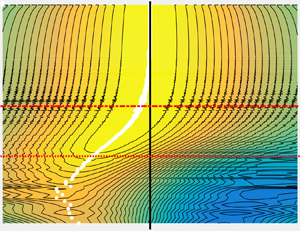
Contours of the correlation coefficient for energy and transfer fluctuations between a selected wavenumber $(k_1\eta \approx 0.02)$ in the IR and another wavenumber ($k_2$) with varying time lags $(\tau )$ are shown in figure 4, for the highest ${R_\lambda }$. Consistent with observations in figure 1, fluctuations in energy of $k_1$ for the full signal are well correlated with those at all wavenumbers in figure 4(a), and are so with no discernible time lag; this strong correlation is present even in the BR and NDR. This feature suggests that the energy across wavenumbers is synchronized. We do not observe in figure 4(a) any significant improvement in correlations with increasing time lag in the IR.

Figure 4. Contours of correlations at different time lags $\tau$ for $E$ and $T$ at a typical low wavenumber $(k_1\eta \approx 0.02)$ with fluctuations at other wavenumbers $k_2$ for ${R_\lambda }\sim 390$. Shown are correlations for (a,b) the full signals and (c,d) those for their slow components. The horizontal lines are the same as the vertical lines in figure 2. The vertical solid line marks zero lag. The contour levels range from $-0.6$ to $1$ with a constant difference of $0.04$.

One possible explanation for the observed synchronicity is the following. The fluctuations of the kinetic energy around their mean value are related to higher-order spectra, associated with fourth-order correlations, etc. Such quantities have been investigated multiple times in the past (Van Atta & Wyngaard Reference Van Atta and Wyngaard1975; Nelkin & Tabor Reference Nelkin and Tabor1990; Praskovsky et al. Reference Praskovsky, Gledzer, Karyakin and Zhou1993). The relevant observation for us is that $E_{uu}(k)$, the spectrum of fluctuations of the kinetic energy around their mean value, also scales as $E_{uu}(k)\sim u_{rms}^2 E(k)$. This corresponds to a sweeping-dominated scaling (Kraichnan Reference Kraichnan1977). Such sweeping implies that the typical temporal behaviour of the spectrum will follow the fluctuations of the velocity, a point we explore in the last section.

This result is contrary to the expectation based on the traditional cascade scenario in which the best correlation would occur with a finite time lag that increases with the wavenumber. On the other hand, the contours shown in figure 4(c) suggest that slower wavenumbers are better correlated with increasing time separation, $\tau$. The maximum correlation is indicated using white dots. Slow fluctuations in $E$ at one value of $k$ in the IR are best correlated with slow fluctuations in another value of $k$ in $E$ when the lag time $\tau$ increases; this suggests, for slow fluctuations, a picture that is consistent with the Kolmogorov–Richardson cascade with finite speed.

This synchronous feature is even stronger for energy transfer, shown in figure 4(b,d), with an interesting behaviour of the peak correlation as one moves to smaller scales. In the IR, the peak correlation of transfer fluctuations with those at large scales is significantly enhanced compared to the full signal. Further, the peak correlation is observed at later times for higher $k_2$. In the BR, the peak correlation is weaker but the increase in lag is more marked than in the IR, up to $k_2\eta \approx 0.3$, beyond which the peak occurs at a constant lag time of about 1.5 eddy turnover times. This suggests that the slow modes adhere most to a cascade scenario in the IR followed by a seemingly synchronized response of the dissipative ranges. One may speculate that fast fluctuations may well be the result of incomplete cancellation of averages over individual triads in wavenumber shells and correspond to instantaneous transfer. This may be important in models that attempt to capture temporal dynamics assuming only a local scale-by-scale transfer. In the NDR, the peak correlation is independent of the scale.

To address the ${R_\lambda }$ trend of the features observed above, we plot the maximum correlation $(\rho _{max})$ for the full signals and the slow-frequency components of $T$ in figure 5(a,b) for three ${R_\lambda }$ and a fixed $k_1\eta$. Figure 5(a) shows correlations from full signals and figure 5(b) from slow fluctuations only. We show the correlations between fluctuations at all $k_2\geq k_1$ for two different $k_1$, one in the IR (dashed lines) and another in the BR (solid lines). In these figures, a high correlation between disparate wavenumbers does not necessarily mean a non-local interaction as the peak correlation may occur with a lag.

Figure 5. The maximum correlation coefficient $(\rho _{max})$ between (a) full and (b) slow modes of energy transfer functions. Dashed lines correspond to $k_1\eta \approx 0.06$ and solid lines to $k_1\eta \approx 0.2$. (c) Time lag corresponding to $\rho _{max}$ in (b). (d) Maximum correlation coefficient $\rho _{max}$ for $k_1\eta \approx 2$. Vertical lines are the same as in figure 2.

It is immediately evident that stronger correlations occur at higher ${R_\lambda }$ for a given pair of $k_1$ and $k_2$, but the figures reveal other features worth discussing. For the full signal, figure 5(a) shows that the fluctuations in $T$ at all $k_2$ are largely uncorrelated with fluctuations when $k_1$ is in the IR. In fact, the correlation drops steeply from a $\rho _{max}$ of 1 when $k_1\neq k_2$. For $k_1$ in the BR, stronger correlations are observed at all $k_2$. For $k_2\eta >0.3$, the peak correlation is independent of the wavenumber. Together with earlier observations, the fact that the peak correlation time in this range is also independent of $k_2$ shows that fluctuations in these scales are synchronized across wavenumbers.

The corresponding correlations for slow transfer fluctuations are shown in figure 5(b). These correspond to white dots in figure 4 and they confirm the ${R_\lambda }$ trend seen in figure 5(a). A comparison of figures 5(a) and 5(b) shows that slow fluctuations are correlated much more strongly than the full signals. The effect of fast fluctuations is thus to reduce the correlation between signals. This reduction effect is stronger at lower ${R_\lambda }$.

For $k_1$ in the IR, the reduction in correlation with $k_2$ $(k_2\neq k_1)$ is weaker for the slow part than for the full signal. The correlation decays up to $k_2\eta \approx 0.3$, beyond which it remains constant. The constant value is significantly larger than that for the full-signal correlations. This feature again highlights that correlations between slow fluctuations are stronger for slow signals, particularly in the transfer. Wavenumbers in the BR are almost perfectly correlated in slow modes.

A similar analysis for fluctuations in $E$ confirms that fluctuations are highly correlated across all wavenumbers with no significant ${R_\lambda }$ trends. We have therefore not shown those data here.

Returning to figure 4, especially figure 4(d) for slow fluctuations, we saw that changes in $E$ and $T$ at large scales are highly correlated with changes at smaller scales, up to the NDR, with a time lag. This time lag increases with the distance between the scales being considered. As noted earlier, this is qualitatively consistent with classical cascade concepts. Note that the slope of the white markers in figure 4(c,d) can be interpreted as the ‘speed’ of the transfer across scales. This information can be used to further our comparison to the classical cascade more quantitatively. The time scale associated with a scale $1/k$ can be estimated by knowing that its energy content is $E(k)k$. Dimensional analysis would then yield $T_c\propto 1/\sqrt {E(k)k^3}$, where $T_c$ is the local time scale associated with $1/k$. In classical phenomenology, this is also the time associated with the transfer of energy to neighbouring smaller scales. In the IR, if $E(k)=C_k\langle \epsilon \rangle ^{2/3}k^{-5/3}$, we obtain $T_c\approx C_k^{-1/2}\langle \epsilon \rangle ^{-1/3}k^{-2/3}$, where $C_k\approx 1.6\text {--}1.7$ (Sreenivasan Reference Sreenivasan1995; Donzis & Sreenivasan Reference Donzis and Sreenivasan2010). Finally, the total time taken by a perturbation in $k_1$ to reach $k_2$ would be the sum of all time intervals to cross the wavenumber interval. If wavenumbers are binned in octaves, for example, the total time is a sum of $T_c$ across different bins (Tennekes & Lumley Reference Tennekes and Lumley1972; Lumley Reference Lumley1992). If one considers a continuum spectrum instead, one obtains

(4.1)\begin{equation} \tau_{k1\to k_2}=\int_{k_1}^{k_2}|\,\textrm{d} T_c/\textrm{d} k| \,\textrm{d} k = C_k^{-1/2}\langle\epsilon\rangle^{-1/3}k_1^{-2/3} \left(1-\left({k_1/k_2}\right)^{2/3} \right). \end{equation}

This can be normalized by the local cascade time scale $T_c(k_1)\approx C_1 T_E$, where $C_1$ is a proportionality constant of order unity relating $T_E$ and $T_c$ when $k_1$ is near the large scales. Then

(4.2)\begin{equation} \frac{\tau_{k_1\to k_2}}{T_E}=C_1\left(1-\left({k_1/k_2}\right)^{2/3}\right). \end{equation}

This expression (also derived by Bos, Shao & Bertoglio (Reference Bos, Shao and Bertoglio2007)) is compared against $\tau _{max}$ in figure 5(c), where the transfer fluctuations peak at later times with increase in $k_2$ within the IR. The measured lag times agree reasonably well with the expression (4.2) for $C_1=1.7$, shown as a dashed black line. Such a behaviour is in contrast to the full signal for which there is no readily identifiable time lag, as discussed earlier. This observation further supports the conclusion that the classical cascade occurs only for the slow signals. As noted earlier, for $k_2\eta >0.3$ – that is, beyond the BR – in the energy transfer spectrum, we have a different behaviour in which the peak correlation is independent of wavenumber. These results are consistent with the results reported in Cardesa et al. (Reference Cardesa, Vela-Martín, Dong and Jiménez2015) and Meneveau & Lund (Reference Meneveau and Lund1994) where the authors studied the correlation between the subgrid-scale stress tensor for velocity fields filtered at different spatial subgrid scales.

The peak correlations for the FDR with a wavenumber in the NDR, shown in figure 5(d), lose the correlation rapidly in both energy and transfer fluctuations. The concept of cascade is not expected to be valid here as the scales are dominated by dissipation. These scales also show large fluctuations that oscillate rapidly. In addition, they are fully correlated with each other as confirmed in figure 1 by the constant correlation in figure 4 and figure 5(d) for ${R_\lambda }>10$ and $k_2\eta \geq 6$. We note that the loss of correlation with increase in $k_2$ for all wavenumbers is only observed for ${R_\lambda }<10$. This again emphasizes that the loss of correlation may be a low-${R_\lambda }$ feature. At higher ${R_\lambda }$, the correlation becomes approximately independent of $k_2$ in the FDR.

Finally, we comment on the relation between transfer and energy fluctuations at the same wavenumber. Because of the differential relation (3.1) between $E$ and $T$, temporal changes in $T(k,t)$ will lead to temporal changes in $E(k,t)$ only after some delay. As a complement to the analysis above, one can look at the peak correlation between $T(k_1,t)$ and $E(k_1,t+\tau )$, now at the same wavenumber $k_1 = k_2 = k$. When $k$ is the dissipative region, figure 6 shows that the peak occurs with zero delay but the delay increases in magnitude across the IR (marked by white dots). In other words, when the slow component of energy is transferred to a wavenumber in the IR, it takes longer and longer for that change to be observed in the energy at that same wavenumber. Over that period other energy exchanges to/from that wavenumber can take place, which may explain why signatures of a classical cascade are much clearer for $T$ than for $E$. These to-and-fro exchanges may also explain why the oscillations around the average value are significantly damped out in the energy signals. Needless to say, no such behaviour is observed in the IR for the full signal.

Figure 6. Contours of correlation at different time lags for slow modes of transfer and energy at the same scale $(k_1=k_2=k)$ for ${R_\lambda }\approx 390$. Horizontal lines are the same as the vertical lines in figure 2. Solid black line is zero lag.