In the following discussion we shall—for the sake of
exposition—use a very simple example to illustrate the issues
involved in model selection and inference post model selection. These
issues, however, clearly persist also in more complicated situations
such as, e.g., nonlinear models, time series models, etc. Consider the
linear regression model
Suppose now that the parameter of interest is the coefficient α
in (1) and that we are undecided whether or not to include the
regressor xt2 in the model a priori. (The
case where a general linear function A(α,β)′,
e.g., a predictor, rather than α is the quantity of interest is
quite similar and is briefly discussed in Remark 4.5.) In other words,
we have to decide on the basis of the data whether to fit the
unrestricted (full) model or the restricted model with β = 0. We
shall denote the two competing candidate models by U and
R (for unrestricted and restricted,
respectively). For any given value of the parameter vector
(α,β), the most parsimonious true model will be denoted by
M0 and is given by
,
respectively. The least-squares estimator for α in the restricted
model will be denoted by
.
We shall decide between the competing models U and R
depending on whether the test statistic
otherwise. This is a traditional pretest procedure based on
the likelihood ratio, but it is worth noting that in the simple example
discussed here it coincides exactly with Akaike's minimum AIC rule
in case
.
(We note here in passing that there is a close connection between
pretest procedures and information criteria in general; see Remark 4.2.)
In fact, in the present example it seems that there is little choice
with regard to the model selection procedure other than the choice of
c, as it is hard to come up with a reasonable model selection
procedure that is not based on the likelihood ratio statistic (at least
asymptotically). Now that we have defined the model selection procedure
,
the resulting post-model-selection estimator for the parameter of interest
α will be denoted by
The following simple observations will be useful: The finite-sample
distribution of
is a convex combination of the conditional distributions, where the
conditioning is on the outcome of the model selection procedure
where Φ(·) denotes the standard normal cumulative
distribution function (c.d.f.). Cf. Leeb and Pötscher (2003a, Sect. 3.1) and Leeb (2003b, Sect. 3.1).
The subsequent discussion is cast in terms of consistent versus
conservative model selection procedures, because this is entrenched
terminology.8
However, despite this
terminology, one should not lose sight of the fact that we are given
only one sample of
in the present example) and we are
interested in the finite-sample properties of this procedure. Any given
model selection procedure can now equally well be embedded as a member
into a sequence of consistent model selection procedures or into a
sequence of conservative procedures for the purpose of asymptotic
analysis (by appropriately defining the model selection procedures at
the other—fictitious—sample sizes). Of course, the
finite-sample properties of the given model selection procedure are
unaffected by our choice of the embedding asymptotic framework. Hence,
when talking about consistent or conservative sequences of model
selection procedures we are in fact not talking about different
procedures but rather about different asymptotic frameworks and their
comparative (dis)advantages in revealing the finite-sample properties
of a given procedure.
2.1. The Consistent Model Selection Framework
As mentioned in the introduction, proceeding with inference post
model selection “as usual” (i.e., as if the selected model
were given a priori) is often defended by the argument that a
consistent model selection procedure has been used and hence
asymptotically the selected model would coincide with the most
parsimonious true model, supposedly allowing one to use the standard
asymptotic results that apply in case of an a priori fixed model. We
now look more closely at the merit of such an argument.
We assume in this section that the cutoff point c in the
definition of the model selection procedure
is chosen to depend on sample size n such that
.
Then it is well known (see Bauer, Pötscher,
and Hackl, 1988; and also Remark 4.3) that the model selection
procedure is a consistent procedure in the sense that
holds for every α, β; i.e., the probability of revealing the
most parsimonious true model tends to unity as sample size increases.
Because the event
is clearly contained in the event
,
the consistency property expressed in (4) moreover immediately entails
that
holds for every α, β, where
denotes the least-squares estimator in the most parsimonious true model.
Although this latter “estimator” is infeasible as it makes
use of the unknown information whether or not β = 0, relation (5)
shows that the post-model-selection estimator
is a feasible version in the sense that both estimators coincide with
probability tending to unity as sample size increases. An immediate
consequence of (5) is that the (pointwise) asymptotic distributions of
are identical, regardless of whether M0 = U
or M0 = R. This latter property, which is
sometimes called the “oracle” property (Fan
and Li, 2001), obviously holds for post-model-selection estimators
obtained through consistent model selection procedures in general; cf.
Pötscher (1991, Lemma 1) for a formal
statement.
9 This property of consistent
model selection procedures has already been observed by Hannan and
Quinn (1979, p. 191). It has since been
rediscovered several times in special instances; cf. Ensor and Newton
(1988, Theorem 2.1); Bunea (2004, Sect. 4).
So far the preceding discussion seems to support the argument that
proceeding “as usual” with inference post consistent model
selection is justified. In particular, it seems to suggest that the
usual construction of confidence sets remains valid post consistent
model selection. Furthermore, observe that (5) entails that the
post-model-selection estimator
is asymptotically normally distributed and is as “efficient”
as the maximum likelihood estimator based on the full model if the full
model is the most parsimonious true model (i.e., if β ≠ 0), and is
more “efficient” (namely, as “efficient” as the
maximum likelihood estimator based on the restricted model) if the
restricted model is the most parsimonious one (i.e., if β = 0).
This seems too good to be true, and, in fact, it is! Although the
result in (5) is mathematically correct, it is a delusion to believe
that it carries much statistical meaning. Before we explore this in
detail, a little reflection shows that the post-model-selection estimator
is nothing else than a variant of Hodges' so-called superefficient
estimator (cf. Lehmann and Casella, 1998, pp.
440–443).
10 Hodges' estimator
(with a = 0 in the notation of Lehmann and
Casella, 1998) is a post-model-selection estimator based on a model
selection procedure that consistently chooses between an N(0,1)
and an N(θ,1) distribution.
It is remarkable that
estimators such as Hodges' estimator, which was constructed in
1951 as an artificial counterexample to the belief that any
asymptotically normally distributed estimator has an asymptotic
variance that can not fall below the (asymptotic)
Cramér–Rao bound, have nowadays come to some prominence in
the guise of post-model-selection estimators based on a consistent
model selection procedure (and of other related estimators; see Section
3). It is equally remarkable that some of the lessons learned from
Hodges' counterexample seem not to have been received in the model
selection literature in the intervening years:
11 Exceptions are Hosoya (1984),
Shibata (1986), Pötscher (1991), and Kabaila (1995,
1996), who explicitly note this
problem.
The actual finite-sample behavior of
is not properly reflected by the (pointwise) asymptotic results;
in fact, these results can be highly misleading regardless of
the sample size and tend to paint an overly optimistic picture of the
performance of the estimator. Mathematically speaking, the culprit is
nonuniformity (w.r.t. the true parameter vector (α,β)) in the
convergence of the finite-sample distributions to the corresponding
asymptotic distributions; cf. the warning already issued in Pötscher
(1991) in the discussion following Lemma 1 and
also in Section 4, Remark (iii), of that paper.
In the simple example discussed here even a finite-sample analysis is
possible that allows us to nicely showcase the problems involved.
12 For a detailed treatment of the
finite-sample properties of post-model-selection estimators in linear
regression models see Leeb and Pötscher (2003a), Leeb (2003a,
2003b).
We begin with a closer look
at the probability
of selecting the most parsimonious true model. From (3) this probability
equals Φ(c) − Φ(−c) if β = 0,
which—in accordance with (4)—goes to unity as sample size
increases because we have assumed c → ∞ in this section.
In case β ≠ 0, the probability equals
and—again in accordance with (4)—converges to unity as
n → ∞. This is so because
,
so that the arguments of the Φ-functions in this formula converge
either both to +∞ or both to −∞. Nevertheless, the
probability of selecting the most parsimonious true model can be very
small for any given sample size if β ≠ 0 is close to
zero. In that case, we see that this probability is close to 1 −
(Φ(c) − Φ(−c)), which in turn
is close to zero because of c → ∞. More precisely,
if β ≠ 0 equals
,
then—despite (4)—the probability of selecting the most
parsimonious true model in fact converges to zero!
13 Slightly more general conditions under which this is true
are given in Proposition A.1 in Appendix A.
That is, the
consistent model selection procedure is completely “blind”
to certain deviations from the restricted model that are of the order
.
In particular, this reveals that the convergence in (4) is decidedly
nonuniform w.r.t. β: In other words, for the asymptotics to
“kick in” in (4) arbitrarily large sample sizes are needed
depending on the value of the parameter β. This means that
,
although being consistent for M0, is not
uniformly consistent (not even locally). (This is in fact true
for any consistent model selection procedure; see Remark 4.4.)
We illustrate
this now numerically. In the following discussion, it proves useful to
write γ as shorthand for
,
i.e., to reparameterize β as
.
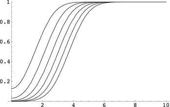
As a function of γ, the probability of selecting the unrestricted
model (which is the most parsimonious true model in case β ≠ 0) is
pictured in Figure 1. Recall that with the choice
our model selection procedure coincides with the minimum BIC method.
Finite-sample model selection probability. The probability of
selecting the unrestricted model as a function of
for various values of n, where we have taken
.
Starting from the top, the curves show
for n = 10k for k =
1,2,…,6. Note that
is independent of α and symmetric around zero in β or,
equivalently, γ.
Figure 1 confirms that the probability of
selecting the correct model can be very small if β ≠ 0 is of the
order
and also suggests that this effect even gets stronger as the sample size
increases. The latter observation is explained by the fact that the
probability of selecting the correct model converges to zero not only
for β ≠ 0 of the order
but even for β ≠ 0 of larger order, namely, for β of the form
;
cf. Proposition A.1 in Appendix A. Furthermore, we can also calculate, for
given β ≠ 0, how many data points are needed such that the
probability of selecting the correct (i.e., the unrestricted) model is at
least 0.9, say. With
as in Figure 1, we obtain: If
β/σβ = 1, then a sample of size n
≥ 8 is needed; if
,
one needs n ≥ 42; if
,
one needs n ≥ 207; and if
,
then n ≥ 977 is required. This demonstrates that the required
sample size heavily depends on the unknown β and increases without
bound as β gets closer to zero.
The phenomenon discussed here occurs only if the parameter β ≠
0 is “small” in absolute value in the sense that it goes to
zero of a certain order.
14 It can be
debated whether the β's giving rise to this phenomenon are
justifiably viewed as “small”: The phenomenon can, e.g.,
arise if β ≠ 0 satisfies
with |ζ| < 1 (cf. Proposition A.1 in Appendix A).
Although such sequences of β's converge to zero by the
assumption
maintained in Section 2.1, the “nonzeroness” of any such
β can be detected with probability approaching unity by a standard
test with fixed significance level or equivalently, with fixed cutoff
point, and thus such β's could justifiably be classified as
“far” from zero. (In more mathematical terms,
Pn,α,β is not contiguous w.r.t.
Pn,α,0 for such β's.) By the
way, this also nicely illustrates that the consistent model selection
procedure is (not surprisingly) less powerful in detecting β ≠ 0
compared with the conservative procedure with a fixed value of
c, the reason being that the consistent procedure has to let
the significance level of the test approach zero to asymptotically
avoid choosing a model that is too large. (This loss of power is not
specific to the consistent model selection procedure discussed here but
is typical for consistent model selection procedures in
general.)
It might then be tempting to argue that in such a
case erroneously selecting the restricted model is not necessarily
detrimental as the restricted model is only “marginally”
misspecified: In particular, the estimator
is consistent, even uniformly consistent (cf. Proposition A.9 in Appendix
A), and satisfies
as n → ∞ (where OP is
understood relative to Pn,α,β for
fixed α and β). However, given that the consistent model
selection procedure is “blind” to deviations from the
restricted model of the order
(and even to deviations of larger order), it should not come as a
surprise that the phenomenon discussed previously crops up again in the
distribution of
.
Recall that, as a consequence of (5),
is asymptotically normally distributed with mean zero and variance equal
to the asymptotic variance of the restricted least-squares estimator if
β = 0 and equal to the asymptotic variance of the unrestricted
least-squares estimator if β ≠ 0. However, in finite
samples—regardless of how large—we get a completely different
picture: From Leeb (2003b), we obtain that the
finite-sample density of
is given by
where φ(·) denotes the standard normal probability
density function (p.d.f.). Furthermore, we have used
Δ(a,b) as shorthand for Φ(a +
b) − Φ(a − b), where Φ
denotes the standard normal c.d.f. Note that
Δ(a,b) is symmetric in its first argument. The
finite-sample density of
does not depend on α and is the sum of two terms: The first
term is the density of
multiplied by the probability of selecting the restricted model. The
second term is a “deformed” version of the density of
,
where the deformation factor is given by the 1 −
Δ(·,·)-term.
15 In light
of (2), the first term is actually the conditional density of
given the event that the pretest does not reject multiplied by the
probability of this event. Because the test statistic is independent of
(Leeb and Pötscher, 2003a, Proposition
3.1), this conditional density reduces to the unconditional one.
Similarly, the second term is the conditional density of
given that the pretest rejects multiplied by the probability of this event.
Because the test statistic is typically correlated with
,
the conditional density is not normal, which is reflected by the
“deformation” factor.
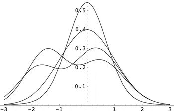
gives an example of the possible shapes of the density of
.
Finite-sample densities. The density
gn,α,β of
for various values of β/σβ. For the graphs,
we have taken n = 100,
,
and σα2 = 1. The four curves correspond to
β/σβ equal to 0, 0.21, 0.25, and 0.5 and are
discussed in the text.
Two of the densities in Figure 2 are
unimodal: The one with the larger mode arises for
β/σβ = 0 and is quite close to the (normal)
density of
corresponding to the restricted model. The reason for this is that the
probability Δ(0,c) of selecting the restricted model is
large, namely, 0.968, and hence the first term in (6) is the dominant
one. The density with the smaller mode arises for
β/σβ = 0.5 and closely resembles the density of
corresponding to the unrestricted model. The reason here is (i) that the
probability of selecting the unrestricted model is large, namely, 0.998,
and hence the second term in (6) is dominant and (ii) that this dominant
term is approximately Gaussian; more precisely, the second term in (6) is
approximately equal to φ(u)(1 − Δ(7 +
0.98u,3)), which differs from φ(u) in absolute value
by less than 0.002. The bimodal densities correspond to the cases
β/σβ = 0.21 and β/σβ =
0.25. In both cases, the left-hand mode reflects the contribution of the
first term in (6) whereas the right-hand mode reflects the contribution of
the second term. The height of the left-hand mode is proportional to the
probability of selecting the restricted model, which is larger for
β/σβ = 0.21 than for
β/σβ = 0.25. In summary, we see that the
finite-sample distribution of
depends heavily on the value of the unknown parameter β
(through β/σβ) and that it is far from its
Gaussian large-sample limit distribution for certain values of β.
The same phenomenon is also found if we repeat the calculations for
other sample sizes n, regardless of how large n is.
In other words: Although the distribution of
is approximately Gaussian for each given (α,β) and
sufficiently large sample size, the amount of data required to achieve
a given accuracy of approximation depends on the unknown β.
In the example presented in Figure 2, a sample
size of 100 appears to be sufficient for the normal approximation
predicted by pointwise asymptotic theory to be reasonably accurate in
the cases β/σβ = 0 and
β/σβ = 0.5, whereas it is clearly
insufficient in case β/σβ = 0.21 or
β/σβ = 0.25.
How can this be reconciled with the result mentioned earlier that
has an asymptotic normal distribution with mean zero and appropriate
variance? The crucial observation again is that this limit result is a
pointwise one; i.e., it holds for each fixed value of the
parameter vector (α,β) individually but does not hold
uniformly w.r.t. (α,β) (in fact, not even locally uniformly):
While it is easy to see that for every
the density gn,α,β(u) given
by (6) converges to the appropriate normal density for each fixed
(α,β), it is equally easy to see (cf. Proposition A.2 in
Appendix A) that (6) has a different asymptotic behavior if, e.g.,
with γ ≠ 0. In this case (6) converges to a shifted
version of the density of the asymptotic distribution of
,
the shift being controlled by γ. Yet another asymptotic behavior
is obtained if we consider
with γn → ∞ (or
γn → −∞) but
γn = o(c). Then
gn,α,β(u) even converges
to zero for every
!
That is, the distribution of
does not “stabilize” as sample size increases
but—loosely speaking—“escapes” to ∞ or
−∞ (depending on the sign of γn);
in fact,
or −∞ in Pn,α,β-probability.
More complicated asymptotic behavior is in fact possible and is described in
Proposition A.2 in Appendix A.
16 A quick
alternative argument showing that the convergence of the finite-sample
c.d.f.s of post-model-selection estimators is typically not uniform
runs as follows: Equip the space of c.d.f.s with a suitable metric
(e.g., a metric that generates the topology of weak convergence).
Observe that the finite-sample c.d.f.s typically depend continuously on
the underlying parameters, whereas their (pointwise) limits typically
are discontinuous in the underlying parameters. This shows that the
convergence can not be uniform.
(To simplify matters the
rather special case ρ
∞ = 0 is excluded from the
preceding discussion; cf. Remark 4.6 for some comments on this case.
However, note that Proposition A.2 also covers the case
ρ
∞ = 0.)
We are now in a position to analyze the actual coverage properties of
confidence intervals that are constructed “as usual,”
thereby ignoring the presence of model selection (this step seemingly
being justified by a reference to (5)). Let
denote the “naive” confidence interval that is given by the
usual confidence interval in the restricted (unrestricted) model if the
restricted (unrestricted) model is selected. That is,
if
and
if
where 1 − η denotes the nominal coverage probability
and zη is the (1 − η/2) quantile of
a standard normal distribution. In view of (2), the actual
coverage probability satisfies
Using the remark in note 15 in the notes section, it is an elementary
calculation to obtain
Note that the coverage probability does not depend on α and is
symmetric around zero as a function of β. Because of (5) and the
attending discussion, pointwise asymptotic theory tells us that the
coverage probability
converges to 1 − η for every (α,β). However, the plots
of the coverage probability given in Figure 3
speak another language.
Finite-sample coverage probabilities. The coverage probability of the
“naive” confidence interval
with nominal confidence level 1 − η = 0.95 as a function of
for various values of n, where we have taken
and ρ = 0.7. The curves are given for n = 10k
for k = 1,2,…,7; larger sample sizes correspond to curves
with a smaller minimal coverage probability.
We see that the actual coverage probability of the
“naive” interval
is often far below its nominal level of 0.95, sometimes falling below 0.3.
Figure 3 also suggests that this phenomenon gets
more pronounced when sample size increases! In fact, it is not difficult to
see that the minimal coverage probability of
converges to zero as sample size increases and not to the nominal coverage
probability 1 − η as one might have hoped for (except possibly in
the relatively special case ρ∞ = 0); cf. also Kabaila
(1995). To see this, note that
where α is arbitrary and γn is chosen
such that γn → ∞ (or
γn → −∞) and
γn = o(c). (The r.h.s. in the
preceding inequality does actually not depend on α in view of
(10).) Because
converges to zero as discussed earlier (cf. Proposition A.1 in Appendix A),
we arrive—using (9) and (10)—at
the last equality being true because
|γn| → ∞ (and because
we have excluded the case ρ∞ = 0).
We finally illustrate the impact of model selection on the (scaled)
bias and the (scaled) mean-squared error of the estimator (again
excluding for simplicity of discussion the case ρ∞
= 0). Let Bias denote the expectation and MSE the
second moment of
.
We discuss the bias first. An explicit formula for the bias can be
obtained from (6) by a tedious but straightforward computation and
is given by
A pointwise (i.e., for fixed (α,β)) asymptotic analysis tells
us that this bias vanishes asymptotically.
17 Although this fits in nicely with (5), it is not a direct
consequence of (5). The crucial point here is that
converges to zero exponentially fast for fixed β ≠ 0; see, e.g.,
Lemma B.1 in Leeb and Pötscher (2003a).
In
Figure
4 we have computed this bias numerically as a function of
.
Note that the bias is independent of α and antisymmetric around
zero in β or, equivalently, γ (and hence is shown only for
γ ≥ 0).
Finite-sample bias. The expectation of
,
i.e., the (scaled) bias of the post-model-selection estimator for α,
as a function of
for various values of n, where we have taken
,
ρ = 0.7, and σα2 = 1. The curves are
given for n = 10k for k =
1,2,…,7; larger sample sizes correspond to curves with larger
maximal absolute biases.
Figure 4 demonstrates that—contrary
to the prediction of pointwise asymptotic theory—the bias can be
quite substantial if β is of the order
and that this effect gets more pronounced as the sample size increases
(the reason for this discrepancy again being nonuniformity in the
pointwise asymptotic results). An asymptotic analysis of (11) using
with γ ≠ 0 shows that the bias converges to
−σα ρ∞γ (see
Proposition A.4 in Appendix A for more information). Note that this
limit corresponds to the “envelope” of the finite-sample
bias curves (for all n) as indicated in Figure 4. Furthermore, if
with γn → ∞ (or
γn → −∞) but
γn = o(c), the asymptotic
analysis in Proposition A.4 even shows that the bias converges to
±∞, the sign depending on the sign of
γn. As a consequence, the maximal absolute bias
in fact grows without bound as sample size increases!
Turning to the MSE we encounter a similar situation. Using
the fact that the test statistic
is independent of
(e.g., Leeb and Pötscher, 2003a,
Proposition 3.1) and that
,
the MSE can be computed explicitly to be
Alternatively, the preceding formula can also be obtained by brute
force integration from the density (6) or from Theorems 2.2 and 4.1 in
Magnus (1999). The MSE is
independent of α. A pointwise asymptotic analysis tells us that
MSE converges to the asymptotic variance
if β = 0 and to the asymptotic variance
if β ≠ 0.
18 Although this is again
in line with (5) it is again not a direct consequence of (5) but follows
from the exponential decay of
for fixed β ≠ 0; cf. note 17. Furthermore, the fact that the
pointwise limit of the MSE coincides with the asymptotic
variance of the infeasible “estimator”
is not particular to the consistent model selection procedure discussed
here. It is true for consistent model selection procedures in general,
provided the probability of selecting an incorrect model converges to
zero sufficiently fast, which is typically the case; see Nishii (1984) for some results in this direction. Of
course, being only pointwise limit results, these results are subject
to the criticism put forward in the present paper.
Again,
however, the finite-sample mean-squared error exhibits a totally
different behavior, regardless how large sample size is (as a result of
nonuniformity in the pointwise asymptotics). This can be gleaned from
Figure 5: The maximal mean-squared error is
much larger than the mean-squared error of the unrestricted
least-squares estimator that is constant and equal to
σ
α2 = 1. As
Figure
5 suggests, the maximal mean-squared error diverges to infinity
as sample size increases, whereas the mean-squared error of
stays bounded (it converges to σα,∞2).
This is well known for the Hodges estimator (e.g., Lehmann and Casella, 1998, p. 442). For the mean-squared
error of
this follows of course immediately from the fact noted previously that
the bias diverges to ±∞ when setting
with γn → ∞ (or
γn → −∞) but
γn = o(c). (The phenomenon
that the maximal absolute bias and hence the maximal mean-squared error
diverge to infinity holds for post-model-selection estimators based on
consistent model selection procedures in general; see Remark 4.1,
Appendix C; and Yang (2003).)
Finite-sample mean-squared error. The second moment of
,
i.e., the (scaled) mean-squared error of the post-model-selection estimator
for α, as a function of
for various values of n, where we have taken
,
ρ = 0.7, and σα2 = 1. The curves are
given for n = 10k for k =
1,2,…,7; larger sample sizes correspond to curves with larger
maximal mean-squared error.
2.2. The Conservative Model Selection Framework
Generally speaking, post-model-selection estimators based on
conservative model selection procedures are subject to phenomena
similar to the ones observed in Section 2.1 for post-model-selection
estimators based on consistent procedures. In particular, the
finite-sample behavior of both types of post-model-selection estimators
is governed by exactly the same formulas, because the finite-sample
behavior is clearly not much impressed by what we fancy about the
behavior of the model selection procedure at fictitious sample sizes
other than n (e.g., what we fancy about the behavior of the
cutoff point c as a function of n). Cf. the
discussion immediately preceding Section 2.1. Not surprisingly, some
differences arise in the asymptotic theory.
In this section we consider the same model selection procedure and
post-model-selection estimator
as before, except that we now assume the cutoff point c to be
independent of sample size n.
19 We
could allow more generally for a sample-size-dependent c that,
e.g., converges to a positive real number. See Leeb and Pötscher
(2003a, Remark 6.2).
This results in a
conservative model selection procedure (that is not consistent).
20 For a detailed treatment of the
finite-sample and asymptotic properties of post-model-selection
estimators based on a conservative model selection procedure see
Pötscher (1991), Leeb and Pötscher
(2003a), and Leeb (2003a, 2003b).
As just noted, the finite-sample distribution, the expectation, and the
second moment of
are again given by (6), (11), and (12), respectively. Also, the
model selection probabilities and the coverage probability of the
“naive” confidence interval are given by the same formulas
as before. As a consequence, all conclusions drawn from the
finite-sample formulas in Section 2.1 remain valid here: The
finite-sample distribution of the post-model-selection estimator is
often decidedly nonnormal, and the standard asymptotic approximations
derived on the presumption of an a priori given model are
inappropriate. In particular, the actual coverage probability of the
“naive” confidence interval is often much smaller than the
nominal coverage probability. Finally, the bias can be substantial, and
the mean-squared error can by far exceed the mean-squared error of the
unrestricted estimator.
We briefly discuss the asymptotic behavior next.
21 Similar as for consistent model selection procedures in
fact all accumulation points of the model selection probabilities, the
finite-sample distributions, the bias, and the mean-squared error can
be characterized by a subsequence argument similar to Remark A.8; cf.
also Leeb and Pötscher (2003a, Remark
4.4(i)), and Leeb (2003b, Remark
5.5).
A much more detailed treatment covering more general
model selection procedures and more general models can be found in
Pötscher (
1991), Leeb and Pötscher
(
2003a), and Leeb (
2003a,
b). The pointwise
limiting behavior of the model selection probabilities can be easily read
off from the finite-sample formula (3):
if
,
reflecting the fact that the model selection procedure is conservative
but not consistent. As in the case of consistent model selection
procedures, this convergence is not uniform w.r.t. β. In contrast
to consistent model selection procedures (cf. Proposition A.1 in
Appendix A), the behavior under sample-size-dependent parameters
(αn,βn) is quite
simple: If
,
then
.
(If
,
then the limit is zero; i.e., the asymptotic behavior is identical to
the asymptotic behavior under fixed β ≠ 0.) In particular, the
asymptotic analysis confirms what we already know from the finite-sample
analysis, namely, that the probability of erroneously selecting the
restricted model can be substantial, namely, if |γ| is
small. However, in contrast to consistent model selection procedures,
this probability does not converge to unity as sample size increases.
It is also interesting to note that deviations from the restricted model
such as
with |ζ| < 1 and cn
→ ∞,
,
that can not be detected by a consistent model selection procedure using
cutoff point cn (cf. Proposition A.1 and note
14 in the notes section) can be detected with probability approaching unity
by a conservative procedure using a fixed cutoff point c.
Consequently and not surprisingly, conservative model selection
procedures are more powerful than consistent model selection procedures
in the sense that they are less likely to erroneously select an
incorrect model for large sample sizes. (Needless to say this advantage
of the conservative procedure is paid for by a larger probability of
selecting an overparameterized model.)
Turning to the post-model-selection estimator
itself, it is obvious that now conditions (4) and (5) are no longer
satisfied;
22 Nevertheless, it is easy to
see that
is consistent (cf. Pötscher, 1991, Lemma 2)
and, in fact, is uniformly consistent; see Proposition B.1 in Appendix
B.
as a consequence, and in contrast to the case of consistent
model selection procedures, the pointwise asymptotic distribution now
captures some of the effects of model selection and no longer coincides
with the usual asymptotic distribution that applies in the absence of model
selection. This can easily be seen from (2): Whereas in the case of
consistent model selection procedures, regardless of the value of β,
only one of the two terms in (2) survives asymptotically and the
corresponding conditioning event becomes a set of probability one
asymptotically and hence has no effect, for conservative procedures both
terms do not vanish in the limit if β = 0. Hence, the pointwise
asymptotic limit captures some of the effects of the model selection step,
at least in the case when the restricted model is correct. (In that sense
the asymptotic framework that views a given model selection procedure as
embedded in a sequence of conservative procedures has some advantage
over the framework considered in Section 2.1.) More precisely, the
pointwise asymptotic distribution of
has a density given by
σα,∞−1φ(u/σα,∞)
if β ≠ 0 and given by
if β = 0. Note that (13) bears some resemblance to the
finite-sample distribution (6). However, the pointwise asymptotic
distribution does not capture all the effects present in the
finite-sample distribution, especially if β ≠ 0; in particular,
the convergence is not uniform w.r.t. β (except in trivial cases
such as ρ∞ = 0); cf. Corollary 5.5 in Leeb and
Pötscher (2003a), Remark 6.6 in Leeb and
Pötscher (2003b), and note 16. A much
better approximation, capturing all the essential features of the
finite-sample distribution, is obtained by the asymptotic distribution
under sample-size dependent parameters
(αn,βn) with
:
This asymptotic distribution has a density of the form
This follows either as a special case of Proposition 5.1 of Leeb
(2003b) (cf. also Leeb and
Pötscher, 2003a, Proposition 5.3 and Corollary 5.4) or can
be gleaned directly from (6). (If
,
then the limit has the form
σα,∞−1φ(u/σα,∞).)
23 Here the convergence of the finite-sample
distribution to the asymptotic distribution is w.r.t. total variation
distance.
Observe that (14) follows the same formula as the
finite-sample density (6), except that σ
α and ρ
have been replaced by their respective limits
σ
α,∞ and ρ
∞ and that
has been replaced by γ.
Consider next the asymptotic behavior of the actual coverage
probability of the “naive” confidence interval
given by (7) and (8). The pointwise limit of the actual coverage
probability has been studied in Pötscher (1991, Sect. 3.3). In contrast to the case of
consistent model selection procedures, it turns out to be less than the
nominal coverage probability in case the restricted model is correct.
However, this pointwise asymptotic result, although hinting at the
problem, still gives a much too optimistic picture when compared with
the actual finite-sample coverage probability. The large-sample minimal
coverage probability of the “naive” confidence interval has
been studied in Kabaila and Leeb (2004).
Although it does not equal zero as in the case of consistent model
selection procedures, it turns out to be often much smaller than the
nominal coverage probability 1 − η (as in Figure 3); see Kabaila and Leeb (2004) for more details.
We finally turn to the bias and mean-squared error of
.
Under the sequence of parameters
(αn,βn) with
,
it is readily seen from (11) that the bias converges to
The pointwise asymptotics corresponds to the cases γ = 0 and
γ = ±∞ (with the convention that
±∞Δ(±∞,c) = 0 and
φ(±∞) = 0) and results in a zero limiting bias.
However, the maximal bias can be quite substantial if β is of the
order
.
In contrast to the case of consistent model selection procedures, the
maximal bias does not go to infinity (in absolute value) as n
→ ∞ but remains bounded. (It is perhaps somewhat
ironic—although not surprising—that consistent model
selection procedures that look perfect in a pointwise asymptotic
analysis lead in fact to more heavily distorted post-model-selection
estimators than conservative model selection procedures.) The limiting
mean-squared error under
(αn,βn) as before is
easily seen to be given by
the pointwise asymptotics again corresponding to the cases γ = 0
and γ = ±∞ (with the convention that
∞Δ(±∞,c) = 0 and
±∞φ(±∞) = 0). In contrast to the case of
consistent model selection procedures, the pointwise limit of
MSE captures some (but not all) of the effects of model
selection and hence no longer coincides with the asymptotic variance of
the infeasible “estimator”
.
Also, in contrast to the case of consistent model selection procedures,
the maximal mean-squared error does not go off to infinity as n
→ ∞, but rather it remains bounded; cf. also Remark 4.1.
2.3. Can One Estimate the Distribution of
Post-Model-Selection Estimators?
It transpires from the preceding discussion that the finite-sample
distributions (and also the asymptotic distributions) of
post-model-selection estimators depend on unknown parameters (i.e.,
β in the example discussed in this paper), often in a complicated
fashion. For inference purposes, e.g., for the construction of
confidence sets, estimators for these distributions would be desirable.
Consistent estimators for these distributions can typically be
constructed quite easily, e.g., by suitably replacing unknown
parameters in the large-sample limit distributions by estimators: In
the case of the consistent model selection procedure discussed in
Section 2.1 a consistent estimator for the finite-sample distribution of
is simply given by the normal distribution
N(0,σα2(1 −
ρ2)), i.e., by the distribution of
,
and by N(0,σα2), i.e., by the
distribution of
.
However, recall from Section 2.1 that the finite-sample distribution of
the post-model-selection estimator is not uniformly close to its pointwise
asymptotic limit. Hence the suggested estimator (being identical with
the pointwise asymptotic distribution except for replacing
σα,∞2 and
ρ∞2 by
σα2 and ρ2)
will—although being consistent—not be close to the
finite-sample distribution uniformly in the unknown parameters, thus
providing a rather useless estimator. In the case of conservative model
selection procedures consistent estimators for the finite-sample
distribution of the post-model-selection estimator can also be
constructed from the pointwise asymptotic distribution by suitably
plugging in estimators for unknown quantities; see Leeb and
Pötscher (2003b, 2004). However, again these estimators will be
quite useless for the same reason: As discussed in Section 2.2, the
convergence of the finite-sample distributions to their (pointwise)
large-sample limits is typically not uniform with respect to the
underlying parameters, and there is no reason to believe that this
nonuniformity will disappear when unknown parameter values in the
large-sample limit are replaced by estimators.
A natural reaction to the preceding discussion could be to try the
bootstrap or some related resampling procedure such as, e.g.,
subsampling. Consider first the case of a consistent model selection
procedure. Then, in view of (4) and (5), the bootstrap that resamples
from the residuals of the selected model certainly provides a
consistent estimator for the finite-sample distribution of the
post-model-selection estimator. Note that the consistent estimator
described in the preceding paragraph can be viewed as a (parametric)
bootstrap. The discussion in the previous paragraph then, however,
suggests that such estimators based on the bootstrap (or on other
resampling procedures such as subsampling), despite being consistent,
will be plagued by the nonuniformity issues discussed earlier. Next
consider the case where the model selection procedure is conservative
(but not consistent). Then the bootstrap will typically not even
provide consistent estimators for the finite-sample distribution of the
post-model-selection estimator, as the bootstrap can be shown to stay
random in the limit (Kulperger and Ahmed,
1992; Knight, 1999, Example 3):24
Kilian (1998)
claims the validity of a bootstrap procedure in the context of
autoregressive models that is based on a conservative model selection
procedure. Hansen (2003) makes a similar
claim for a stationary bootstrap procedure in the context of a
conservative model selection procedure. The preceding discussion
intimates that both these claims are at least unsubstantiated.
Basically the only way one can coerce the bootstrap into delivering a
consistent estimator is to resample from a model that has been selected
by an
auxiliary consistent model selection procedure. (The
construction of consistent estimators in Leeb and Pötscher,
2003b,
2004, alluded to
previously basically follows this route.) In contrast, subsampling will
typically deliver consistent estimators. However, the discussion in the
preceding paragraph strongly suggests that any such estimator will
again suffer from the nonuniformity defect.
A natural question then is how estimators (not necessarily derived
from the asymptotic distributions or from resampling considerations)
can be found that do not suffer from the nonuniformity defect. In other
words, we are asking for estimators
of the finite-sample c.d.f.
that are uniformly consistent, i.e., that satisfy for every
and every δ > 0
However, it turns out that no estimator
can satisfy this requirement (except possibly in the trivial case where
ρ∞ = 0). For conservative model selection
procedures this is proved in Leeb and Pötscher (2003a, 2004) in a more
general framework, including model selection by AIC from a quite
arbitrary collection of linear regression models. For a consistent
model selection procedure such a result is given in Leeb and
Pötscher (2002, Sect. 2.3). In fact,
these papers show that the situation is even more dramatic: For every
consistent estimator
even
holds for suitable δ > 0, and this result is even local in the
sense that it holds also if the supremum in the preceding display
extends only over suitable balls that shrink at rate
.
25 Similar “impossibility” results apply to
estimators of the model selection probabilities; see Leeb and
Pötscher (2004) in the case of
conservative procedures; for consistent procedures this argument can be
easily adapted by making use of Proposition A.1.
(These
“impossibility” results hold for randomized estimators of
Gn,α,β also.)
The preceding “impossibility” results establish in
particular that any proposal to estimate the distribution of
post-model-selection estimators by whatever resampling procedure
(bootstrap, subsampling, etc.) is doomed as any such estimator is
necessarily plagued by the nonuniformity defect (if it is consistent at
all). On a more general level, an implication of the preceding results
is that assessing the variability of post-model-selection estimators
(e.g., the construction of valid confidence intervals post model
selection) is a harder problem than perhaps expected.26
The confidence interval suggested in Hjort
and Claeskens (2003, p. 886) does not provide
a solution to this problem. As pointed out in Remark 3.5 of Kabaila and
Leeb (2004), the proposed interval
(asymptotically) coincides with the classical confidence interval
obtained from the overall model.