3.1. Definition of heading

Heading, sometimes called yaw or azimuth, is one of three rotational degrees of freedom, which is natural to define for land, sea, and air navigation, due to the direction of gravity. By heading, we mean the orientation about the vertical direction vector (where vertical is defined as the normal to the reference ellipsoid). The heading can be represented in several ways, e.g. as a scalar, such as in the Euler angles roll, pitch and yaw (which have singularities at certain positions/orientationsFootnote ¹ ). Heading can also be represented by a rotation matrix or quaternion containing the full orientation. How the heading is represented is not important for this paper, since the discussion is valid for any representation.

3.2. Categorising methods for heading estimation

When investigating the various methods for heading estimation, it turns out that for each method, a vector is utilised to find the heading. It is also clear that different methods use different vectors, and based on this it seems sensible to define different categories of methods based on which vector is used.

Following this system, we find that there are seven different vectors in common use in practical navigation systems, and thus we define seven corresponding methods. The seven methods are presented in Section 4.

3.3. Basic principles of heading calculation

The vector used to find heading (or orientation in the general case) is denoted by $\vec x$ . The vector must have a known (or measurable) direction relative to the Earth (E) and for now we assume that also the length is known, such that ${{\bi x}^E}$ is known. We also need to know the vector relative to the vehicle (B), i.e. ${{\bi x}^B}$ . The relation between these vectors is

(1) $${{\bi x}^E} = {{\bi R}_{EB}}{{\bi x}^B}$$

where we want to calculate ${{\bi R}_{EB}}$ , the vehicle orientation. Note that the length of $\vec x$ is not needed to find ${{\bi R}_{EB}}$ , it is sufficient to know the direction of ${{\bi x}^E}$ and ${{\bi x}^B}$ (if the lengths are unknown, unit vectors can be used).

Of the three degrees of freedom in ${{\bi R}_{EB}}$ , it is not possible to find the orientation about an axis parallel to $\vec x$ by using Equation (1), but the two remaining degrees of freedom are determined. For example, the gravity vector is known relative to E (when the position is approximately known) and for a stationary vehicle, it is measured relative to B by accelerometers. This gives roll and pitch, while heading (rotation about the gravity vectorFootnote ² ) is not found. To find the heading we thus need a vector with a non-zero horizontal component, i.e.

(2) $${\vec x_{horizontal}} \ne \vec 0$$

3.4. Accuracy of the heading calculation

In practice there will be errors in the knowledge about both ${{\bi x}^E}$ and ${{\bi x}^B}$ , and we can write

(3) $$\eqalign{& {\hat{\hskip -2pt \bi x}}_E^E = {{\bi x}^E} + \delta {\bi x}_E^E \cr & {\hat{\hskip -2pt \bi x}}_B^B = {{ \bi x}^B} + \delta {\bi x}_B^B} $$

where the hat indicates a quantity with error. ${{\bi x}^E}$ and ${{\bi x}^B}$ are the true vectors and the delta-terms are the error vectors. The subscript E shows that the error originates from determining $\vec x$ in E, and similarly for subscript B. In coordinate free form Equation (3) can be written

(4) $$\eqalign{&{\hat {\vec x}}_E = \vec x + \overrightarrow {\delta {x_E}} \cr & {\hat {\vec x}}_B = \vec x + \overrightarrow {\delta {x_B}}} $$

Note that the two error-vectors, $\overrightarrow {\delta {x_E}} $ and $\overrightarrow {\delta {x_B}} $ are generally not correlated, as they originate from different calculations/measurements. $\overrightarrow {\delta {x_B}} $ is often an error from an on-board (internal) sensor, while $\overrightarrow {\delta {x_E}} $ usually is given by error in external information. Both errors will contribute to the final heading error, but their relative importance will vary greatly between the seven methods, and this will be discussed for each method in Section 4.

Only the components of the error-vectors that are both horizontal and normal to $\vec x$ will contribute to the heading error (when assuming small angular errors). If we let the operator ()_contr return the length of the contributing component, we can write the standard deviation of these contributing errors $\sigma \left( {{{(\overrightarrow {\delta {x_E}} )}_{contr}}} \right)$ and $\sigma \left( {{{(\overrightarrow {\delta {x_B}} )}_{contr}}} \right)\!$ . The standard deviation of the resulting heading error (δψ) is then given by (uncorrelated errors assumed, first order approximation)

(5) $$\sigma \left( {\delta \psi} \right) \approx \displaystyle{{\sqrt {\sigma {{\left( {{{(\overrightarrow {\delta {x_E}} )}_{contr}}} \right)}^2} + \sigma {{\left( {{{(\overrightarrow {\delta {x_B}} )}_{contr}}} \right)}^2}}} \over {\left \vert {{{\vec x}_{horizontal}}} \right \vert}} $$

4.1. Method 1: The magnetic vector field of the Earth

The most basic method for finding heading is probably by means of a magnetic compass. For any position of B, the (total) magnetic vector field will give a vector ${\vec m_B}$ (this vector is determined by the position of B, in contrast to the kinematical vectors in Table 2 that are constructed from a relation between two coordinate frames). A magnetometer can measure the direction (relative to B) of the magnetic vector with high accuracy, thus ${\bi m}_B^B $ is accurately found (and the error contribution from $\overrightarrow {\delta {x_B}} $ is small). However, the magnetic vector at the position of the magnetometer will have contributions from other sources than the known (and relatively weak) magnetic field of the Earth, and in many cases there will be a large uncertainty in ${\bi m}_B^E $ (i.e. the contribution from $\overrightarrow {\delta {x_E}} $ is significant). In addition, ${\vec x_{horizontal}}$ will be short at high latitudes (far north or south).

While the predictable global declination can be compensated for quite easily (e.g. by the International Geomagnetic Reference Field model (IAGA, 2010)), local deviations often limit the practical accuracy of a magnetic compass. Naturally occurring magnetic material in the ground can give deviations of tens of degrees (Leaman, Reference Leaman1997; Langley, Reference Langley2003), and similar magnitudes of error are also common in urban areas (Godha et al., Reference Godha, Petovello and Lachapelle2005). Vehicles travelling at a significant distance from the ground, e.g. in air or deep water, are far less vulnerable to these deviations, but their compass may still be degraded by other effects, such as rapid changes in the solar wind. Geomagnetic storms give greatest distortion at higher latitudes, but can sometimes also give significant errors at medium latitudes, such as a 7° change during 20 hours in Scotland (Thomson et al., Reference Thomson, McKay, Clarke and Reay2005).

Ferrous materials or electromagnetic interference from the vehicle itself may give significant errors due to the short distance to the compass. The static part of these may be corrected for by calibration procedures, but contributions from changes in the vehicle's magnetic signature (e.g. from changing electrical currents) must still be considered (Healey et al., Reference Healey, An and Marco1998). Some key properties of Method 1 are summarised in Table 4.

Table 4. Method 1 (magnetic compass), some key properties.

4.2. Method 2: The angular velocity of the Earth

The second vector to consider is the angular velocity of the Earth relative to inertial space, ${\vec \omega _{IE}}$ . In contrast to the previous method, the direction of this vector is very well known in E, and it defines the locations of the geographic North- and South Pole. Hence the error from $\overrightarrow {\delta {x_E}} $ is usually negligible.

One possible way to find ${\bi \omega} _{IE}^B $ is by means of a camera that is detecting change in the direction to celestial objects, e.g. the apparent movement of stars is mainly given by ${\vec \omega _{IE}}$ for an Earth-fixed camera. However, in practical navigation ${\bi \omega} _{IE}^B $ is usually measured by means of gyroscopes, and the method is thus called gyrocompassing. For the rest of this section we will assume that gyroscopes are used to find ${\bi \omega} _{IE}^B $ (usually ring laser, fibre optic or spinning mass gyros).

The uncertainty of this method is dominated by $\overrightarrow {\delta {x_B}} $ , i.e. error in ${\bi \omega} _{IE}^B $ . The vector ${\bi \omega} _{IE}^B $ is found from the relation

(6) $${\bi \omega} _{IE}^B = {\bi \omega} _{IB}^B - {\bi \omega} _{EB}^B. $$

The first term ( ${\bi \omega} _{IB}^B $ ) is measured by the gyros, and for stationary scenarios ( ${\vec \omega _{EB}}(t) = \vec 0\;\forall \;t$ ) the gyro error is the main error source. In such scenarios, the gyro error can be averaged to improve the heading accuracy (the ideal averaging time is given by the bottom point of the Allan variance plot (Allan, Reference Allan1966) of the gyro). The constant part of the gyro error can be cancelled if the gyros can be mechanically rotated, e.g. rotating 180° about the down-axis. This can be very useful e.g. for MEMS gyros, which typically have large constant biases, and thus rotation can make gyrocompassing possible (Renkoski, Reference Renkoski2008; Iozan et al., Reference Iozan, Kirkko-Jaakkola, Collin, Takala and Rusu2010). How different carouseling schemes affect the heading accuracy is discussed in Renkoski (Reference Renkoski2008). Rotation to improve the heading accuracy can also be obtained by turning the vehicle, when feasible.

For a moving vehicle, gyrocompassing is more challenging since ${\bi \omega} _{EB}^B $ (the second term of Equation (6)) usually has a significant uncertainty. Using a strapdown IMU and knowledge of the vehicle's velocity ( $\vec v_{\underline{E} B}^{} $ ), the heading can still be found by utilising the movement of the gravity vector relative to inertial space, as shown in Figure 1.

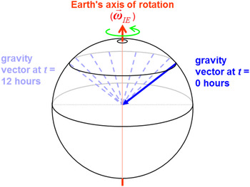
Figure 1. The gravity vector will rotate relative to the inertial space (figure assumes low/zero velocity relative to Earth).

The length of ${\vec x_{horizontal}}$ will obviously decrease at higher latitudes, and from geometry and Equation (5) we see that the uncertainty of Method 2 will be proportional to 1/cos(latitude), and the accuracy of marine gyrocompasses is often in the order of 0·1°/cos(latitude). In Table 5 a short (simplified) summary of Method 2 is given.

Table 5. Method 2 (gyrocompassing), some key properties.

4.3. Method 3: Vector between external objects

In the third method, heading is obtained by observing at least two objects (O₁ and O₂), that form a vector ${\vec p_{{O_1}{O_2}}}$ . If the global positions of the two objects are known, the vector is known in E, ${\bi p}_{{O_1}{O_2}}^E $ . Finding the direction of ${\bi p}_{{O_1}{O_2}}^B $ may be done with a camera (with known orientation relative to the vehicle), e.g. a downward-looking camera in an Unmanned Aerial Vehicle (UAV) recognising O₁ and O₂. A feature with a known direction, such as a building or a road, may also be recognised and used, but here we simply consider it to consist of one or more vectors known in E. The sensor does not need to be a camera; the principle can also be used by other imaging sensors such as a sonar (Lucido et al., Reference Lucido, Pesquet-Popescu, Opderbecke, Rigaud, Deriche, Zhang, Costa and Larzabal1998).

To find heading, ${\vec p_{{O_1}{O_2}}}$ must obviously have a horizontal component, but the direction of observation does not need to be vertical. Consider the concept of leading lights (range lights) for ships, i.e. one low and one high lighthouse that are vertically aligned when the ship is positioned at the correct bearing. In this case ${\vec p_{{O_1}{O_2}}}$ points directly towards (or away from) the ship, and the direction of ${\bi p}_{{O_1}{O_2}}^B $ is easily found e.g. by means of an alidade or a camera.

This method can also be used with celestial objects, such as the stars, where the direction of ${\bi p}_{{O_1}{O_2}}^E $ will be known when time is known. Star trackers are commonly used to determine the orientation of spacecraft, but can also be used from the surface of Earth (Samaan et al., Reference Samaan, Mortari and Junkins2008).

For Method 3, a high heading accuracy can be obtained from one pair of objects, and with more than two objects, the accuracy will improve further. An example of star tracker accuracy is 0·02° (around boresight, Dzamba et al., Reference Dzamba, Enright, Sinclair, Amankwah, Votel, Jovanovic and McVittie2014). The method is summarised in Table 6.

Table 6. Method 3 (vector between external objects), some key properties.

4.4. Method 4: Vector from own vehicle to external object

Methods 1 to 3 may work without knowing the vehicle's own position, but for the rest of the methods, knowledge about vehicle position (or change in position) is needed for the heading calculation. The first of these methods is related to Method 3, but with the knowledge of vehicle (B) position, only one external object O is needed, i.e. we use the vector $\vec p_{BO}^{} $ . When we also know the position of O, ${\bi p}_{BO}^E $ is found. The direction of the horizontal part of $\vec p_{BO}^{} $ relative to the vehicle's orientation is often called the bearing of the object, and when the bearing is measured, we have the needed part of ${\bi p}_{BO}^B $ .

To measure the bearing in practice, a camera may be used, recognising an object in the picture. There are also other possibilities, e.g. a radio transmitter with a known position can be used as the object, if bearing can be measured by the receiving antenna. Underwater, hydrophones can measure the bearing to an acoustic transmitter or a river outlet with known position.

The object used does not need to be Earth-fixed, as long as the position of the object is known, such that we can determine the direction of ${\bi p}_{BO}^E $ . A relevant example is when a second vehicle is travelling close enough to be observed, and the position of that vehicle can be received through a communication channel. A similar situation (that is most relevant on land) is when a GNSS receiver is placed in an observable position, a procedure that is used e.g. to determine the heading of instruments for land surveying (Leica Geosystems, 2008) and for aiming (Rockwell Collins, 2015).

Celestial objects usually have a known position relative to Earth when time is known, and are thus suitable for Method 4, e.g. the direction to the Sun or a satellite transmitting radio signals can be used to find the heading when own position is known (unless when directly above, where ${\vec x_{horizontal}} = \vec 0$ ). An example where heading is estimated with an accuracy of about 1° by means of the Sun is found in Lalonde et al. (Reference Lalonde, Narasimhan and Efros2010).

If three or more different objects (with different horizontal bearings) are available for observation, horizontal position of B can first be calculated (the “Snellius-Pothenot Surveying Problem” (Dorrie, Reference Dorrie1965)), and subsequently any of the objects can be used to find the heading (using $\vec p_{BO}^{} $ ). Some key properties of Method 4 are summarised in Table 7.

Table 7. Method 4 (vector from vehicle to object), some key properties.

4.5. Method 5: Body-fixed vector

The two previous methods were using ${\vec p_{{O_1}{O_2}}}$ and $\vec p_{BO}^{} $ , and thus it is now natural to look at the vector ${\vec p_{{B_1}{B_2}}}$ , i.e. using two separate positions B ₁ and B ₂ on the vehicle. If we can measure the position of both B ₁ and B ₂ e.g. from two GNSS receivers or other means, ${\bi p}_{{B_1}{B_2}}^E $ is found. ${\bi p}_{{B_1}{B_2}}^B $ is typically known from the mounting (and it is constant when assuming a rigid body).

In the example of two GNSS-receivers, heading can be found with two independent receivers if the baseline ( ${\vec x_{horizontal}}$ ) is sufficiently large. However, ${\bi p}_{{B_1}{B_2}}^E $ can be found much more accurately (allowing a shorter baseline), by utilising the phase difference of the GNSS carrier signal at two (or more) antennae (resolving the integer ambiguities). An accuracy of about 0·3° can be achieved with a baseline of 0·5 m (Hemisphere GNSS, 2015).

The ${\vec p_{{B_1}{B_2}}}$ -method can also be used without GNSS, consider e.g. an upward looking camera at ground level with known orientation, observing both B ₁ and B ₂ (e.g. two recognisable lights) at a vehicle flying above the camera. A similar example is given in Hauschild et al. (Reference Hauschild, Steigenberger and Rodriguez-Solano2012) where the heading of a satellite, which has two transmitting antennae with a baseline of 1·3 m, was estimated. Ground stations can measure the phase difference of the waves from the two antennae, and can thus estimate the direction of ${\bi p}_{{B_1}{B_2}}^E $ .

For Method 5, $\overrightarrow {\delta {x_B}} $ is usually found accurately by measurements of the installed B ₁ and B ₂ at the vehicle, and if the vehicle is sufficiently rigid, this error will be small. $\overrightarrow {\delta {x_E}} $ will typically be larger, but a long baseline can make the resulting heading error very small, giving the method a high potential accuracy. A short summary of Method 5 is given in Table 8.

Table 8. Method 5 (multi-antenna GNSS/body-fixed vector), some key properties.

4.6. Method 6: Vehicle velocity vector

So far, the methods have been independent of own movement, but if the vehicle has a horizontal velocity component, the velocity vector ${\vec v_{\underline{E} B}}$ can also be used to find heading.

Finding ${\bi v}_{\underline{E} B}^B $ can be done in several ways, where one option is using a Doppler sensor, such as an underwater acoustic Doppler velocity log or a Doppler radar. One or more cameras can also be used, where the optical flow of Earth-fixed features is tracked (Zinner et al., Reference Zinner, Schmidt and Wolf1989; Sivalingam and Hagen, Reference Sivalingam and Hagen2012). Sensors that measure velocity relative to water or air may also be used if sea current or wind is known (or small relative to ${\vec v_{\underline{E} B}}$ ). Finally, ${\bi v}_{\underline{E} B}^B $ can also be found from knowledge of the vehicle movement, e.g. a vehicle on rails or wheels may have a restricted movement such that

(7) $${\bi v}_{\underline{E} B}^B \approx \left[ {\matrix{ x \cr 0 \cr 0 \cr}} \right]\comma$$

where x is the forward speed (and hence the course equals the heading). For vehicles in air/water, an aerodynamic/hydrodynamic model may be used to calculate velocity relative to the surrounding air/water.

For Method 6 to work, we also need ${\bi v}_{\underline{E} B}^E $ , which can be obtained from GNSS (utilising Doppler shift or carrier phase (van Graas and Soloviev, Reference van Graas and Soloviev2004). If position measurements ( ${\bi p}_{EB}^E $ ) are available, ${\bi v}_{\underline{E} B}^E $ can in theory be found by direct differentiation. In practice, a correctly designed integrated navigation system will use Method 6 to estimate heading when position measurements and ${\bi v}_{\underline{E} B}^B $ are available. An example is the navigation system of the HUGIN Autonomous Underwater Vehicle (AUV), where Method 6 is necessary to find heading with the required accuracy for vehicles that are not equipped with high-accuracy gyros (Gade and Jalving, Reference Gade and Jalving1998). The method gives a heading accuracy of about 0·5° when ${\bi p}_{EB}^E $ is regularly transmitted to the AUV from a surface ship (that has found ${\bi p}_{EB}^E $ by combining acoustic relative positioning and GNSS), since the AUV has a Doppler velocity log and under normal operation has a horizontal velocity component.

The accuracy of method 6 will clearly increase with higher horizontal speed, while the two errors $\overrightarrow {\delta {x_E}} $ and $\overrightarrow {\delta {x_B}} $ typically will originate from two different sensors, and which of them is dominating will depend on the given scenario. Some key properties of Method 6 are summarised in Table 9.

Table 9. Method 6 (velocity vector), some key properties.

4.7. Method 7: Vehicle acceleration vector

Method 6 required a sensor measuring ${\bi v}_{\underline{E} B}^B $ (or sufficient knowledge about this vector), which for many navigation systems will not be available. However, almost every navigation system will have accelerometers, and thus we can instead find the vector ${\bi a}_{\underline{E} B}^B $ (after subtracting the contribution from the gravity and Coriolis force). Hence, if the vehicle has a horizontal acceleration component, ${\vec a_{\underline{E} B}}$ can be used to find heading. Obtaining ${\bi a}_{\underline{E} B}^E $ can be done similarly as in Method 6, i.e. by getting measurements of ${\bi v}_{\underline{E} B}^E $ or ${\bi p}_{EB}^E $ , typically from GNSS.

FFI has investigated the accuracy of this method when using MEMS IMUs, by comparing the heading calculated from Method 7 with the heading from two rigidly attached references. The first reference is Honeywell HG9900 IMU (gyro biases of only 0·003°/h), from which the estimator in the navigation software NavLab (Gade, Reference Gade2005) will find heading accurately using Method 2. The second reference is a camera, where heading is found by Method 4 each time a picture is taken, as shown in Figure 2.

Figure 2. Verifying Method 7 by Method 4, from helicopter. NavLab has calculated the orientation and position of the camera when the picture was taken, giving a direction vector. The position where the direction vector intersects an available terrain model is compared with the centre of the picture taken.

In a helicopter doing turns, ${\vec a_{\underline{E} B}}$ is large, and heading is found accurately from Method 7. By using Sensonor STIM300 IMU and GPS position aiding, NavLab (with smoothing) obtained a heading accuracy of 0·16° (1σ). This accuracy was found by measuring the deviation in 26 pictures (and it is in accordance with both the deviation from the HG9900-reference and the theoretical uncertainty reported by the NavLab estimator).

A lower acceleration will obviously reduce the accuracy (due to shorter ${\vec x_{horizontal}}$ ), but by aiding NavLab with ${\bi v}_{\underline{E} B}^E $ instead of ${\bi p}_{EB}^E $ , less acceleration, with shorter duration is needed to find heading. This is because the integrated acceleration can be distinguished more quickly from the noise in ${\bi v}_{\underline{E} B}^E $ than that in ${\bi p}_{EB}^E $ , since the latter requires a second integration.

FFI has looked at the accuracy available from Method 7 in a car, and Figure 3 shows the result from a test where ${\bi a}_{\underline{E} B}^E $ is found from ${\bi p}_{EB}^E $ and from two variants of ${\bi v}_{\underline{E} B}^E $ .

Figure 3. The heading accuracy from Method 7 in the car test varied with acceleration and with different methods to find ${\bi a}_{\underline{E} B}^E $ . The car had a stationary period before driving on smaller roads, and then a period on a highway, before driving back the same way. The three graphs show theoretical uncertainty in smoothed heading when NavLab is aided with GPS position ( ${\bi p}_{EB}^E $ ) or GPS velocity ( ${\bi v}_{\underline{E} B}^E $ ) from Doppler shift or carrier phase. Only the uncertainty with GPS position aiding is verified with an external heading reference, the two others are simulated with accuracies based on u-blox (2015) and van Graas and Soloviev (Reference van Graas and Soloviev2004).

Method 7 is summarised in Table 10.

Table 10. Method 7 (acceleration vector), some key properties.

4.8. Other methods

Seven different vectors that are all widely used to find heading have been presented. However, given all the different applications around the globe that find orientation, we cannot guarantee that all methods in use are covered among the seven, but we think the most important ones are included. Appendix B will briefly discuss some possible methods not covered by the seven, but to our knowledge, they are in little or no use in practical navigation.